HAL Id: tel-01996088
https://hal.laas.fr/tel-01996088
Submitted on 28 Jan 2019HAL is a multi-disciplinary open access archive for the deposit and dissemination of sci-entific research documents, whether they are pub-lished or not. The documents may come from teaching and research institutions in France or abroad, or from public or private research centers.
L’archive ouverte pluridisciplinaire HAL, est destinée au dépôt et à la diffusion de documents scientifiques de niveau recherche, publiés ou non, émanant des établissements d’enseignement et de recherche français ou étrangers, des laboratoires publics ou privés.
Kinodynamic motion planning for quadrotor-like aerial
robots
Alexandre Boeuf
To cite this version:
Alexandre Boeuf. Kinodynamic motion planning for quadrotor-like aerial robots. Automatic. Institut national polytechnique de Toulouse (INPT), 2017. English. �tel-01996088�
THÈSE
THÈSE
En vue de l’obtention duDOCTORAT DE L’UNIVERSITÉ FÉDÉRALE
TOULOUSE MIDI-PYRÉNÉES
Délivré par :
l’Institut National Polytechnique de Toulouse (INP Toulouse)
Présentée et soutenue le 05/07/2017 par :
Alexandre BOEUF
KINODYNAMIC MOTION PLANNING FOR QUADROTOR-LIKE AERIAL ROBOTS
JURY
Rachid ALAMI Directeur de Recherche Examinateur
Marilena VENDITTELLI Professeur associé Examinateur
Thierry FRAICHARD Chargé de Recherche Rapporteur
Paolo ROBUFFO GIORDANO
Directeur de Recherche Rapporteur
Thierry SIMÉON Directeur de Recherche Directeur de thèse
Juan CORTÉS Directeur de Recherche Directeur de thèse
École doctorale et spécialité :
MITT : Domaine STIC : Intelligence Artificielle
Unité de Recherche :
Laboratoire d’analyse et d’architecture des systèmes
Directeur(s) de Thèse :
Thierry SIMÉON et Juan CORTÉS
Rapporteurs :
Contents
Introduction 1
1 Motion planning: main concepts and state of the art 5
1.1 General notions . . . 5
1.1.1 Modeling the system . . . 5
1.1.2 Problem formulation and configuration space . . . 6
1.1.3 The planning methods . . . 7
1.2 Sampling-based motion planning . . . 8
1.2.1 Overview . . . 8
1.2.2 Main components . . . 9
1.2.3 Probabilistic roadmaps . . . 11
1.2.4 Diffusion-based methods . . . 14
1.3 Kinodynamic motion planning . . . 18
1.3.1 Problem formulation . . . 18
1.3.2 Decoupled approach . . . 19
1.3.3 Direct planning . . . 20
1.4 Motion planning for aerial robots . . . 26
1.4.1 Trajectory generation . . . 26
1.4.2 Planning in the workspace . . . 27
1.4.3 Decoupled approach . . . 27
1.4.4 Finite-State Motion Model: The Maneuver Automaton . . . . 28
2 Modeling and motion control of a quadrotor 29 2.1 Quadrotor dynamics model . . . 29
2.2 Motion control of a quadrotor . . . 31
2.2.1 A brief introduction to control theory . . . 31
2.2.2 Control space and state space of a quadrotor . . . 32
2.3 Physical constraints . . . 33
2.3.1 In the space of the thrust forces amplitudes . . . 34
2.3.2 In the control space . . . 34
2.4 Differential flatness . . . 37
3 Steering method for a quadrotor 39 3.1 A two-point boundary value problem . . . 40
3.1.1 Definition of the full problem . . . 40
3.1.2 Independence of the outputs . . . 41
3.2 A near time-optimal spline-based approach . . . 43
3.2.1 Closed-form solution . . . 43
3.2.2 Duration of the phases . . . 46
ii Contents
3.2.4 Synchronization . . . 47
3.2.5 Generalization to other robotic systems . . . 48
3.3 Discussion on optimality . . . 48
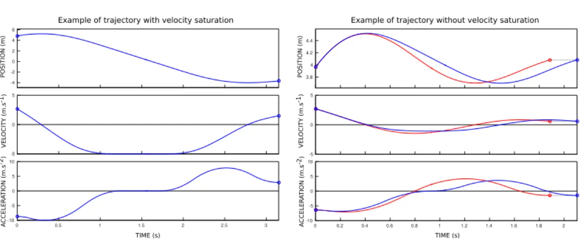
3.3.1 Optimality and velocity saturation . . . 48
3.3.2 In one dimension . . . 49
3.3.3 In three dimensions . . . 51
4 Kinodynamic motion planning for a quadrotor 55 4.1 A decoupled approach . . . 55
4.1.1 From path to trajectory . . . 56
4.1.2 Optimization . . . 57
4.2 Direct kinodynamic planning . . . 58
4.2.1 Quasi-metric in the state space . . . 58
4.2.2 Sampling strategy . . . 61
4.2.3 Global methods for kinodynamic planning . . . 66
4.2.4 Experimental results . . . 67
5 Experimental work 71 5.1 Geometric tracking controller on SE(3) . . . . 71
5.1.1 Overview . . . 72
5.1.2 Trajectory tracking . . . 72
5.1.3 Attitude tracking . . . 73
5.2 ART: the Aerial Robotics Testbed . . . 73
5.2.1 Hardware . . . 74
5.2.2 Software . . . 74
5.3 Experimentation . . . 79
5.3.1 Set-up . . . 79
5.3.2 Results . . . 80
6 Integration into the ARCAS project 83 6.1 The ARCAS project . . . 83
6.1.1 Overview . . . 83
6.1.2 Consortium . . . 84
6.1.3 Objectives . . . 85
6.1.4 The ARCAS system . . . 86
6.2 The motion planning system . . . 88
6.2.1 Navigation . . . 88
6.2.2 Transportation for a single ARM . . . 89
6.2.3 Coordinated transportation and manipulation . . . 89
6.3 Symbolic-Geometric planning to ensure plan feasibility . . . 91
6.3.1 Geometric Task Planner . . . 92
6.3.2 Tasks: decomposition and implementation . . . 93
Contents iii
A Calculation details of the steering method 99 A.1 Reminders . . . 99 A.2 Expression of the spline . . . 101 A.3 Durations of the phases . . . 101
Introduction
Motion planning is the field of computer science that aims at developing algorithmic techniques allowing the automatic computation of trajectories for a mechanical system. The nature of such a system will vary according to the fields of application. In computer animation for instance this system could be a humanoid avatar. In molecular biology it could be a protein. The field of application of this work being robotics, the system is here a robot. We define a robot as a mechanical agent controlled by a computer program. The modern meaning of the word seems to come from the English translation of the 1920 play R.U.R. (Rossum’s Universal Robots), by Karel Capek, from Czech, robotnik (slave) derived from robota (forced labor). As for the term robotics (the science of robots), it was first used by Isaac Asimov in the 1941 short story Liar! The main feature of a robot is its ability to interact with its environment through motion. Being able to efficiently plan its movements is therefore a fundamental component of any robotic system.
More specifically we will focus here on aerial robotics, i.e. flying robots. Histor-ically the first term used to refer to a remotely operated aircraft was drone (male bee). According to the military historian Steven Zaloga it was the American Com-mander Delmer Fahrney that first used it in homage to the British remote-control bi-plan DH 82B Queen Bee. However, since a flying robot is not necessarily remotely controlled, we will use in this work the term UAV (Unmanned Aerial Vehicles). Also note that not all UAVs are robots since a UAV could very well be remotely con-trolled by a human operator instead of a computer program. Aerial robotics has a wild range of applications. Apart from the sadly famous military ones, we can cite photography and video, inspection, surveillance, search and rescue, and even aerial manipulation as we will see later. For these civilian applications a class of devices is more and more used because of its scalability, agility, and robustness: the multi-rotor helicopters. In this work we will focus on the four-rotor kind called
quadrotor or sometimes quadcopter.
The classic motion planning problem consists in computing a series of motions that brings the system from a given initial configuration to a desired final configu-ration without generating collisions with its environment, most of the time known in advance. Usual methods typically explore the system’s configuration space re-gardless of its dynamics. By construction the thrust force that allows a quadrotor to fly is tangential to its attitude which implies that not every motion can be per-formed. This could, for example, be compared to the fact that a car can not move sideways. Furthermore, the magnitude of this thrust force is limited by the physical capabilities of the engines operating the propellers. Therefore the same applies to the linear acceleration of the robot. For all these reasons, not only position and orientation must be planned, higher derivatives must be planned also if the motion is to be executed. When this is the case we talk of kinodynamic motion planning.
2 Contents
In motion planning a distinction is usually made between the local planner and the global planner. The former is in charge of producing a valid trajectory between two configurations (or states) of the system without necessarily taking collisions into account. The later is the overall algorithmic process that is in charge of solving the motion planning problem by exploring the configuration space (or the state space) of the system. It relies on multiple calls to the local planner. The first contribution of this thesis is to propose a local planner that interpolates two states consisting of an arbitrary number of degrees of freedom (dof) and their first and second derivatives. Given a set of bounds on the dof derivatives up to the fourth order (snap), it quickly produces a near-optimal minimum time trajectory that respects those bounds. Although in the context of this thesis this local planner is applied to the quadrotor system which state is considered to be its flat outputs (the 3D position of the center of mass and the yaw angle) together with their first and second derivatives, it can more generally be applied to any system with either uncoupled dynamics or that is differentially flat.
In most of modern global motion planning algorithms, the exploration is guided by a distance function (or metric) and some of these algorithms are very sensible to it. The best choice is often to use the cost-to-go, i.e. the cost associated to the local method. For instance if the configuration space is an Euclidean space and the local method is the linear interpolation then the best metric is the Euclidean distance since it is also the cost-to-go. But in the context of kinodynamic motion planning, the cost-to-go is often the duration of the minimal-time trajectory. The problem in this case is that computing the cost-to-go is as hard (and thus as costly) as computing the optimal trajectory itself. The second contribution of this thesis is to propose the use of a specific metric that is a good approximation of the cost-to-go but which computation is far less time consuming.
The dominant paradigm in motion planning nowadays is sampling-based motion
planning. This class of algorithms relies on random sampling of the configuration
space (or state space) in order to quickly explore it. Several different strategies can be considered. A common sampling strategy is for instance uniform sampling. However, for some types of constrained problems this choice may not be the most efficient. It appears that in our context uniform sampling is in fact a rather poor strategy. We will indeed see that a great majority of uniformly sampled states can not be interpolated. The third contribution of this thesis is an incremental sampling strategy that significantly decreases the probability of this happening.
Please note that this work has been realized in the context of the European funded project ARCAS (Aerial Robotics Cooperative Assembly System) that has been conducted between the years 2012 and 2016 and that proposed the develop-ment and experidevelop-mental validation of the first cooperative free-flying robot system for assembly and structure construction. It paved the way for a large number of applications including the building of platforms for evacuation of people or land-ing aircrafts, the inspection and maintenance of facilities and the construction of
Contents 3
structures in inaccessible sites and in space. The fourth contribution of this the-sis is, through this project, the demonstration that an interface between symbolic and geometric planning, previously developed at LAAS-CNRS, can successfully be applied to aerial manipulation.
This document is organized as follows:
In Chapter 1 we introduce the general concepts used in motion planning along with a state of the art of there applications to robotics. We then do the same with kinodynamic motion planning. We finally provide an overview of the state of the art of motion planning in the context of aerial robotics.
The focus of Chapter 2 is the quadrotor system itself. We first give a model of its dynamics which in a second time allows us, after a brief introduction to the general principles of control theory, to define its control space and its state space. Its physical constraints in the control space are then discussed. We finally see that the system is differentially flat, which is having an impact on planning.
In Chapter 3 we focus on our proposition of steering method for a quadrotor. We first present the corresponding two-point boundary value problem. A method to solve it, that can be used as a local planner, is then proposed. It is a near time-optimal spline-based approach for which we will discuss the optimality of the computed solutions. We finally see how this method can be applied to more general systems.
In Chapter 4 we present the global approaches on which we have focused to solve the kinodynamic motion planning problem for a quadrotor. We show in particular how our local planner can be integrated into those global methods. We first present a decoupled approach together with a local optimization method of the global solution trajectory. We then focus on direct approaches. In that perspective we begin by addressing the problem of the metric in the state space. Follows the description of an incremental sampling strategy in the state space. We finally present two global direct approaches to kinodynamic motion planning and discuss the influence of both the metric and the sampling strategy on both of them.
The goal of Chapter 5 is to show that the trajectories that we plan using the methods described in Chapters 3 and 4 can actually be executed on a real physical system. We first present the controller we have chosen to track our trajectories. We then give an overview of our testbed: its different components, both in terms of hardware and software, and how they interconnect. We finally present the con-ducted experiments together with some of their results.
In Chapter 6 we detail the integration of our works into the ARCAS project in the context of which they were conducted. We first present the project itself, its objectives, its different partners, its subsystems and the general framework in which they are integrated. We then focus on the motion planning system and finally detail the link between symbolic and geometric planning.
Chapter 1
Motion planning: main
concepts and state of the art
Contents
1.1 General notions . . . . 5
1.1.1 Modeling the system . . . 5
1.1.2 Problem formulation and configuration space . . . 6
1.1.3 The planning methods . . . 7
1.2 Sampling-based motion planning . . . . 8
1.2.1 Overview . . . 8
1.2.2 Main components . . . 9
1.2.3 Probabilistic roadmaps . . . 11
1.2.4 Diffusion-based methods . . . 14
1.3 Kinodynamic motion planning . . . . 18
1.3.1 Problem formulation . . . 18
1.3.2 Decoupled approach . . . 19
1.3.3 Direct planning . . . 20
1.4 Motion planning for aerial robots . . . . 26
1.4.1 Trajectory generation . . . 26
1.4.2 Planning in the workspace . . . 27
1.4.3 Decoupled approach . . . 27
1.4.4 Finite-State Motion Model: The Maneuver Automaton . . . . 28
In this chapter we introduce the general concepts used in motion planning along with a state of the art of there applications to robotics and then more specifically to aerial robotics.
1.1
General notions
1.1.1 Modeling the system
As an introduction we stated that motion planning is the field of computer science that aims at developing algorithmic techniques allowing the automatic computation
6 Chapter 1. Motion planning: main concepts and state of the art
of trajectories for a mechanical system. The classical way of modeling such a system is to use a kinematic chain. It consists of a set of rigid bodies called links. A rigid body is a closed subset B of the workspace W, i.e. the space where motion takes place. Usually the workspace is the three dimensional Euclidean space R3. Links can be connected to each others. These connections are called joints. They are modeled as ideal movements between links such as relative rotations and translations. Note that any joint can be modeled as a set of rotations and translations. For example the so called free-flying joint which represents the unconstrained motion of a rigid body in the three dimensional Euclidean space R3 with respect to a given inertial frame is modeled by three translations and three rotations. Note that this is the case for a quadrotor when not considering differential constraints on the motion. This formalism provides a natural parametrization of a kinematic chain. Indeed, if every numerical value of the angles of rotation and displacements in translation are known then the geometrical state of the system in the workspace is entirely defined. A given set of such values, represented by a tuple of real numbers, is called a configuration, often noted q. One element of the tuple is called a degree of freedom (dof) and therefore the number of parameters (the length of the tuple) is referred to as the number of dof of the kinematic chain. The next section gives the formulation of the motion planning problem in this context.
1.1.2 Problem formulation and configuration space
The classic formulation of the motion planning problem is known as the piano
movers’ problem [Schwartz 1983]. It can be stated as follows: “Given a kinematic
chain and a set of rigid bodies considered as obstacles which positions and orien-tations are known, is there a continuous collision-free motion that will take the kinematic chain from a given initial collision-free configuration to a desired final collision-free configuration?”. Note that the original formulation was actually given for a system composed of only a single free-flying body. This more complete for-mulation is known as the generalized mover’s problem [Reif 1979].
In 1983, Tomas Lozano-Péres introduced the use in robotics of the previously known notion of configuration space [Lozano-Pérez 1983], often noted C. It is defined as the set of all possible configurations of a kinematic chain. Its topological nature and dimension depends on the system. For example the configuration space of a free-flying rigid body is the special Euclidean group of dimension three, SE(3). An other classic example is the double pendulum which configuration space is the 2-torus, C = S1×S1= T2 (see Figure 1.1). In any case, C is a n-dimensional manifold,
with n the number of dof of the chain. Given a kinematic chain and a set of obstacles in W, we can define the subset Cobst⊆ C as the set of configurations in collision. We then define the free space and note Cf ree = C \ Cobst its complementary subset in C,
i.e. the set of collision-free configurations. This representation has the advantage
of reducing the motion planning problem to the search of a continuous path for a point in Cf ree. Formally the problem becomes the one of finding a continuous
1.1. General notions 7
application τ : [0 1] → Cf ree such that τ (0) = qinit and τ (1) = qf inal, where
qinit and qf inal are the initial and final configurations of the system respectively. Solving the problem with this formulation consists in studying the connectivity of the free space. Indeed, a solution exists if and only if qinit and qf inalare in the same connected component of Cf ree. In the next section we present the main approaches that have been developed to tackle this problem.
Figure 1.1: The double pendulum and its configuration space the 2-torus.
1.1.3 The planning methods
Even if the earliest works on motion planning date back from the late 60’s [Nilsson 1969], most of the algorithmic works started in the early 80’s. Numer-ous approaches have been developed over this last three decades. One can classify them into two main subsets: the complete methods and the other ones. A method is said to be complete when it is able not only to find a solution if one exists but also to determine the (non-)existence of solutions. These methods often rely on an explicit representation of Cf ree which is a problem that has been shown to be polynomial in the number of obstacles but exponential in the number of degrees of freedom (i.e. the dimension of the problem) [Reif 1979]. And this is indeed the complexity of the most efficient of them [Canny 1988a]. This practical inability to scale to real-life applications is the reason why these methods are bound to only have a theoretical interest.
Exploring the connectivity of Cf ree without having to explicitly represent it has been a motivation for the development of other methods. Some of them rely on a comprehensive discretization of Cf ree[Faverjon 1984, Lozano-Perez 1987] using cells or grids. They are said to be resolution complete. This means that if a solution exists, then there is a discretization resolution for which these methods are able to find it. Because the higher the problem’s dimension goes the finer the required resolution becomes, the number of cells or grids tends to rapidly become quite big. These methods are therefore also unable to perform in reasonable time in high dimension.
8 Chapter 1. Motion planning: main concepts and state of the art
Other classes of methods are using the potential field approach [Khatib 1986, Koren 1991]. The idea is to define a potential field other the configuration space which is the sum of an attractive field generated by the goal configuration and repulsing fields generated by the obstacles (i.e. the elements of Cobst). An opti-mization process based on gradient descent techniques is then performed other this field. These techniques have good performances even in high dimension and are par-ticularly well suited to tackle reactive obstacle avoidance problems. They however have a week spot which is their tendency to quickly get trapped into local minima of the potential field. The use of random walks [Barraquand 1990, Barraquand 1991] has been introduced to overcome this limitation, thus opening the way to sampling-based motion planning, which is the focus of our next section. Note that a more ex-tensive overview of all these motion planning techniques can be found in Latombe’s book [Latombe 2012].
1.2
Sampling-based motion planning
1.2.1 Overview
In the potential field method, the introduction of random walks as a tool to escape local minima opened the way to the use of sampling-based approaches in motion planning. But randomness here only plays its part when the main process gets stuck. What if exploration of the connectivity of Cf ree could be achieved mainly through the use of randomness? This idea, inherited from the Monte Carlo method [Metropolis 1949], is behind sampling-based motion planning. The general principle consists in randomly sampling configurations in C and dismiss the ones in Cobstwith collision checking algorithms. This way, we get a discretization of Cf ree without having to explicitly represent it. If the sampling is uniform then as the number of samples increases the discretization itself becomes more and more uniform. This technique provides an efficient way to explore Cf ree but not its connectivity. To do that, the sampled configuration have to be linked inside a network of valid tran-sitions between them. And this is the heart of sampling-based motion planning: what strategies should be used to try and link the sampled collision-free configura-tions? Many different approaches have been developed over the years, which can be divided into two main families: the probabilistic networks and the diffusion-based methods. See Figure1.2 for an illustration of typical behaviors of these methods. All these techniques have in common the fact that they are probabilistically
com-plete, meaning that if a solution exists then it can be found given enough computing
time. This section provides a presentation of the main components of these methods along with a description of some of the existing variants for each two main families. We will also introduce the concept of sampling-based kinodynamic planning needed to tackle the differential constraints imposed by some systems such as the quadro-tor. Note that a more comprehensive overview of sampling-based motion planning
1.2. Sampling-based motion planning 9
techniques can be found in LaValle’s book [LaValle 2006].
Figure 1.2: An illustration of typical behaviors of a probabilistic roadmap method (a) compared to a diffusion-based approach (b)
1.2.2 Main components
Sampling-based motion planning explores the connectivity of Cf reeby sampling ran-dom configurations and trying to connect them within a feasible transition network. Thus to represent this underlying network a data structure is needed. A natural candidate is the graph structure often called a roadmap. A node represents a con-figuration and an edge represents a valid transition between two concon-figurations. Several things have to be noted here.
We assumed up to now that the configuration sampling was uniform. This is not necessarily the case. Uniform sampling is actually only one sampling strategy among many other possibilities. As we will see in sections 1.2.3 and 4.2.2, the sampling strategy can have a significant influence on the overall performances of a motion planning algorithm.
We say that an edge represents a valid transition between configurations. What is the nature of this transition, how is it computed and what does valid means in this context? When we talk of a transition between two configurations qi and qj, we actually refer to a continuous path in C which end points are these configurations. It is called a local path, as opposition to the global solution of the motion planning problem. It is computed by the steering method (also called the local planner). Formally, this method can be thought as a deterministic application
SM : C 2 → C0([0 1], C) (qi, qj) 7→ SMij ! s.t. ( SMij(0) = qi SMij(1) = qj (1.1)
where C0([0 1], C) is the set of continuous applications from [0 1] to C. The simplest
(and therefore most commonly used) steering method is linear interpolation:
10 Chapter 1. Motion planning: main concepts and state of the art
Note that in this case SM is symmetric, meaning that:
∀(qi, qj) ∈ C2, ∀u ∈ [0 1], SMij(u) = SMji(1 − u) (1.2)
When this is the case the underlying graph is undirected. But a steering method is not necessarily symmetric as we will see in chapter 3, in which case the graph has to be directed.
As for what valid means, in the classic formulation of the piano movers’ problem for instance it stands for collision-free. Note that the local path does not indeed necessarily lie in Cf ree. This has to be a posteriori verified by the collision checking
module. But collisions are not always the only constraints. For some robots, not
every path in the free space can be executed. For example a car-like robot is not able to move sideways. Thus the local paths produced by the steering method also have to be feasible to be valid. In the example of the car-like robot, the system is said to be non holonomic. It means that the equations of motion are non integrable differential equations involving the time derivatives of the configuration variables. This is often the case when the system has less controls than configuration vari-ables. For instance a car-like robot has two controls (linear and angular velocity) while its configuration space is of dimension three (position and orientation in the plane). Planning for non holonomic systems can sometimes be treated by carefully choosing a specifically designed steering method ([Dubins 1957]). A more compre-hensive discussion on the subject can be found in [Laumond 1998]. Non holonomy thus implies kinematic constraints arising from the underlying dynamics of the sys-tem. But an other type of constraints can arise from dynamics. A system can be submitted for example to maximum velocity or acceleration because of its physical limitations. More generally a differential constraint is a bound on the modulus of the time derivatives of the degrees of freedom of the system. Planning collision-free trajectories for such systems implies to take into account both the kinematic con-straints (collisions and possibly non holonomy) and the dynamics concon-straints. This is called the kinodynamic motion planning problem [Canny 1988b, Donald 1993]. Kinodynamic motion planning will be detailed in section 1.3.
We still have to mention a crucial component. When a new collision-free con-figuration is sampled the way it is tried to be linked to the current graph is called the connection strategy. It is the algorithmic core specific to each method and re-sponsible for managing calls to the steering method. Designing such a strategy mainly consists in choosing what connections are to be tested and in which order. The following sections present two main families of connection strategies and their variants.
At that stage, either to increase efficiency in probabilistic roadmaps, or to guide the exploration towards empty regions in diffusion-based methods, a nearest neigh-bours search is often performed in order to select candidate nodes in the current graph and the order in which they should be considered. In this case, the definition
1.2. Sampling-based motion planning 11
of a metric (or distance function) on the configuration space is needed. It is an application M : C2 → R+ such that:
∀(qi, qj, qk) ∈ C3, M (qi, qj) = 0 =⇒ qi = qj : coincidence M (qi, qj) = M (qj, qi) : symmetry M (qi, qk) ≤ M (qi, qj) + M (qj, qk) : triangle inequality The most commonly used metric is the Euclidean metric ME(qi, qj) = kqi− qjk2.
But this is not always the case. For car-like robots for intense the metric has to be related to the steering method, or even induced by it (see for instance [Laumond 1993, Giordano 2006]). Note that as discussed by [LaValle 2001] the ideal metric is the cost-to-go, i.e. for a given cost function the cost of bringing the system from qi to qj. The problem is that finding the cost-to-go is often as hard as solving the planning problem. It is therefore often important to find a good and computationally efficient approximation. Also note that if the cost-to-go is not symmetric neither is the ideal distance function. The ideal metric would then be a quasi-metric, which has the same properties of a metric, symmetry excepted. A more comprehensive discussion on this issue will be conducted in section 4.2.1. The next section presents a family of connection strategies known as the probabilistic
roadmaps.
1.2.3 Probabilistic roadmaps
The first version of this connection strategy was first introduced by [Kavraki 1996] under the name Probabilistic Roadmap Method (PRM). It since gave birth to many variants. This strategy consists in two phases: a learning phase and a query phase. During the learning phase the connectivity of the free space is explored and stored in a graph as explained in the previous section. Note that this method was the first to use the idea of capturing the connectivity of the free space in a graph. The query phase consists in connecting the initial and final configurations to the graph and then perform a shortest path search.
During the learning phase described in Algorithm 1, the undirected graph G is stored in a set N of nodes and a set E of edges both initially empty. At each iteration a random configuration q is sampled. If q is not in collision then it is added to N and a set Nq of nearest neighbors of q in N is selected according to a given metric M and a threshold (possibly infinite, i.e. Nq= N ). For each node n in Nq, and if n and q are not already connected in G (i.e. if n and q are not in the same connected component of G), the local path SM (q, n) is computed and tested for collisions. If it is collision free then the edge (q, n) is added to E and the connected components of G are updated. The algorithm runs until a chosen learning time has passed.
For an initial configuration qi and a final configuration qf, the query phase consists in finding two nodes ni and nf in N such that ni and nf are in the same
12 Chapter 1. Motion planning: main concepts and state of the art
Algorithm 1: PRM learning phase
N ← ∅; E ← ∅; G ← {N, E};
while time < learning time do
q ← random configuration;
if q ∈ Cf ree then
N ← N ∪ {q};
Nq← NearestNeighbors(q, N );
foreach n ∈Nq in increasing order of M (q, n) do if n and q not in same connected component then
if SM (q, n) is valid then E ← E ∪ {(q, n)}; UpdateConnectedComponents(G) ; end end end end end Return G;
connected component of G and both SM (qi, ni) and SM (qf, nf) are collision free. This is done the same way a new random configuration is added at each step of the learning phase. The query fails if no such nodes can be found. In this case an other learning phase if performed. Otherwise a shortest path search is conducted in G between qi and qf using for examples either a A∗ or Dijkstra algorithm.
Learning the connectivity of the free space before making a planning query and then keeping this information between each next query is the reason why this method is particularly well suited for multiple planning queries for the same system in the same static environment. The class of methods inspired by PRM are thus often called multiple queries methods. Note however that this approach can be used in a single query mode. It is for example possible to initialize the node set with
N = {qi} (instead of N = ∅) and choose qf as the first configuration to add (instead of a random one). In this case the algorithm stops when qi and qf are in the same connected component of G (or when a given amount of time has passed).
Many variants of this method have been proposed since in order to try and in-crease the overall efficiency of the planning process. Some of them are targeting one well established drawback that is the difficulty of finding connections going through the thiner regions of the free space. This is known as the narrow passage problem. It is a consequence of the uniform sampling strategy of the configuration space. In regions where Cobst is dense, a poor coverage of the free space is indeed obtained when using uniform sampling. Therefore some approaches are using different
sam-1.2. Sampling-based motion planning 13
pling strategies. A class of methods is increasing the probability of finding samples in Cf ree by targeting the border of Cobst. One possibility is to allow some of the samples to lie in Cobst and then try to “push” them towards Cf ree [Hsu 1998]. In the
Obstacle-Based PRM approach [Amato 1998], the opposite strategy is implemented:
samples lying in Cf reeare “pushed” towards Cobst. In the Gaussian sampling strategy [Boor 1999] couples of close configurations are sampled and disregarded if one of them does not lie in Cobst while the other lies in Cf ree. A different class of methods are adopting the opposite approach, namely trying to generate samples as far away from Cobst as possible by sampling the generalized Voronoi diagram of Cf ree (also called the medial-axis) [Wilmarth 1999, Lien 2003].
Note that as announced in section 1.2.2 we can see that different sampling strate-gies can be used and that they have a significant impact on the overall performances of a motion planning algorithm. In section 4.2.2 we propose a sampling strategy of our own designed to increase the efficiency of motion planning for a quadrotor.
Another drawback of random sampling is that it is not trivial to esti-mate the coverage quality of the free space. In the Visibility-PRM algorithm [Nissoux 1999, Siméon 2000], a simple on-line estimation of the proportion of the hyper-volume of the free space covered by the roadmap is proposed. With this information one can design a better stop condition for the learning phase than a maximum number of iteration or computing time. In this approach a sample is added to the roadmap only if it can be used to merge together two connected com-ponents or is not “visible” by any other node. The coverage estimation is then a function of the number of consecutive unsuitable sampled configurations. This approach has also the advantage of generating a roadmap containing fewer nodes, thus decreasing the number of local paths to be computed and therefore speeding up each iteration. Note that it also tackles very well the narrow passage problem.
Some methods are trying to increase efficiency by decreasing the number of calls to the collision checking module. Collision detection is indeed by far the most time consuming process of a classic PRM algorithm (about 90% of computing time [van Geem 2001]). In the Lazy-PRM algorithm [Bohlin 2000] the learning phase is performed without taking into account any of the obstacles. All calls to the collision checking module are done during the query phase, eliminating invalid local paths during the shortest path search. In the Fuzzy-PRM variant [Nielsen 2000], collision detection is performed with an incremental resolution which is leading to an overall decrease of the number of calls to the collision checking module.
Finally, some methods focus on optimality. Up to now we did not mention optimality because it was not relevant when considering the generalized mover’s problem. Efficiently finding a solution if one exists was the only concern. However, aforementioned methods often produce low quality solutions. It has indeed been proven by [Karaman 2011] that a standard PRM does not converge towards the optimal solution. Optimality is relative to a given cost function. For example, length of the global solution path is often considered but some other criteria such
14 Chapter 1. Motion planning: main concepts and state of the art
as clearance to the obstacles can be used. Whatever the considered cost function, a low quality solution can be problematic when trying to execute it on the physical system. A classic way to deal with this issue is to post-process the low quality solutions by means of an optimization method, also called a smoothing method. Examples are numerous but since it is not our point we won’t give any of them here. Note that we will however give an example of smoothing method in section 4.1.2. An other way of dealing with optimality is to consider it while planning. This is is the case of a simplified version of PRM called sPRM, proposed in [Kavraki 1998], which converges towards the optimal. A more efficient proposition called PRM∗was since made by [Karaman 2011]. The next section presents a family of connection strategies known as the diffusion-based methods.
1.2.4 Diffusion-based methods
In this class of methods the underlying structure that is used to explore the free space is a special kind of graph: a tree, i.e. a graph with no cycles in it. More generally the structure is actually a forest, a set of trees. The idea here is to in-crementally build this structure starting from either the initial configuration qinit, the final configuration qend or both. The two main differences with the PRM-based methods is that no learning phase is required and not all Cf ree is explored. The search is indeed usually biased to solve one specific motion planning problem. This class of methods is thus often called single queries methods. A distinction is usually made between unidirectional and multi-directional methods. In the former a single tree is constructed with either qinit or qend as its root until the other configuration is reached. In the latter several trees are constructed. In a bidirectional method in particular, two trees with roots qinit and qend respectively are iteratively con-structed until the two trees meet. These methods are particularly well suited to problems where either or both the initial and final configurations are in a highly constrained region of the free space as it is for example the case in the context of assembly maintainability [Chang 1995]. Choosing between an unidirectional and a bidirectional method usually depends on whether only one of the end configuration is constrained or both.
We have briefly mentioned the Randomized Path Planner (RPP) [Barraquand 1991] already as being the first randomized motion planning al-gorithm. By its use of the concept of random walks, it is also the first approach to diffusion-based methods.
Another approach called the Ariadne’s Clew Algorithm (ACA) was proposed by [Bessiere 1993]. A genetic algorithm is used to generate a tree rooted at qinit while trying to optimize the distribution of its nodes other Cf ree. In a second phase the goal configuration is tried to be linked to the tree.
In the bidirectional approach called Expansive-Space Tree (EST) and proposed by [Hsu 1997, Hsu 2000], the algorithm iteratively executes two steps labeled as
1.2. Sampling-based motion planning 15
expansion and connection respectively. During the expansion step a node is selected
in one of the two trees with a probability inversely proportional to the number of nodes lying in its neighborhood (according to a given metric and threshold). A given number of configurations are then sampled in this given neighborhood of the selected node and tried to be linked to it. The connection step consists in trying to link the newly added nodes to nearby nodes of the other tree.
Nowadays, the most popular diffusion-based method is without a doubt the
Rapidly-exploring Random Tree (RRT) algorithm introduced by [Lavalle 1998].
Al-though initially Al-thought as a tool to solve non-holonomic and kinodynamic mo-tion planning problems (see next secmo-tion) this approach has since been successfully adapted to problems without differential constraints [Kuffner 2000, LaValle 2000]. This method can be used either as unidirectional or bidirectional (or even multi-directional as we will see later). As in EST a construction phase and a connection phase are alternated but both the way the node to be expanded is selected in the tree and the way this expansion is made differ. At each iteration a random config-uration, qrand, is sampled in C. Its nearest configuration in the tree, qnear, is then selected (according to a chosen metric). Given a steering method SM , as defined in (1.1), the local path LP = SM (qnear, qrand) is generated. A node expansion process is then applied to generate a new configuration, qnew, in two possible ways according to the chosen version of the algorithm. For that, a fixed value ε ∈ ]0 1] has been previously set as a parameter of the algorithm. In the classic variant (usually referred to as RRT-Extend) the new configuration is qnew= LP (ε). In the variant called RRT-Connect [Kuffner 2000] the expansion process is iterated as long as qnew is collision free. The expansion process (that we call Expand) is described in Algorithm 2 and illustrated in Figure 1.3 for the Extend version.
Algorithm 2: Node expansion of the RRT algorithm (Expand)
LP ← SM (qnear, qrand);
qnew← LP (ε);
if RRT-Connect then
k ← 2;
while kε ≤ 1 and LP (kε) ∈ Cf ree do
qnew← LP (kε);
k ← k + 1;
end end
Return qnew;
If qnew is collision free, the local path SM (qnear, qnew) is tested for validity. If it is valid, both the node and the edge are added to the tree. The connection phase is then applied. In the unidirectional version the local path SM (qnew, qend) is tested for validity (alternatively SM (qnew, qinit) if the tree is rooted at qend). If it is valid the algorithm stops. In the bidirectional version (that we refer to as
16 Chapter 1. Motion planning: main concepts and state of the art
Figure 1.3: One expansion step of the RRT algorithm for the Extend version.
Bi-RRT) qnew is tried to be linked to nearby nodes in the other tree (as in EST). If one of the attempted connections is successful the algorithms stops. Note that in this bidirectional version each tree is alternatively expanded (as in EST). In a variant referred to as balanced the trees are kept with the same number of nodes. These steps are iterated until a maximum number of iteration has been reached. The unidirectional version of the algorithm is described in Algorithm 3 for a tree rooted at qinit. Algorithm 3: Unidirectional RRT N ← {qinit}; E ← ∅; T ← {N, E}; k ← 0; while k < K do
qrand← random configuration;
qnear ← NearestNeighbor(qrand, N );
qnew← Expand(qnear, qrand);
if qnew ∈ Cf ree and SM (qnear, qnew) is valid then
N ← N ∪ {qnew};
E ← E ∪ {(qnear, qnew)};
if SM (qnew, qend) is valid then
N ← N ∪ {qend}; E ← E ∪ {(qnear, qend)}; Return T ; end end k ← k + 1; end Return T ;
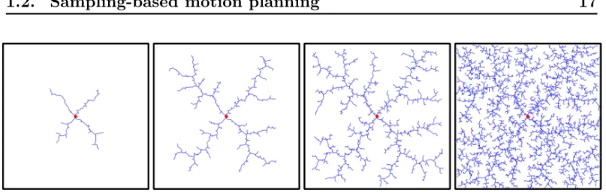
A fundamental property of RRT is the Voronoi biasing. The probability that a node is selected for expansion is proportional of the volume of its Voronoi region. This implies that the algorithm rapidly explore the free space because it favors diffusion towards unexplored regions. Figure 1.4 shows the evolution of a tree constructed by the RRT algorithm and covering the free space.
1.2. Sampling-based motion planning 17
Figure 1.4: Evolution of a tree constructed by the RRT algorithm and covering the free space.
This method has since gave birth to many variants. For instance a lazy bidi-rectional version is proposed by [Sánchez 2003]. Similarly to PRM-based methods, some variants are targeting the sampling strategy. A obstacle-based variant tack-ling the narrow passage problem is proposed by [Rodriguez 2006] while a different approach avoiding the dense regions in proposed by [Khanmohammadi 2008]. In the Dynamic-Domain RRT [Yershova 2005] and its adaptive version [Jaillet 2005], the notion of visibility is used to better refined the sampling domain. Another ap-proach based on dimension reduction uses principal component analysis techniques to better guide the exploration inside narrow passages [Dalibard 2009].
The Exploring/Exploiting Tree algorithm (EET) proposed by [Rickert 2008] is a combination between a potential field approach and a RRT-based approach. Information about the connectivity of the workspace gathered during exploration is exploited to compute a navigation function that defines a potential field. The planner gradually switches to a diffusion-based exploration when the exploitation method fails.
Quality of the solutions is also a concern for the diffusion-based meth-ods. Optimality is asymptotically achieved by the algorithm RRT∗ proposed by [Karaman 2011]. In this version the tree is locally reorganized each time a new node is added. More generally, generating high-quality paths with respect to a cost functional have been investigated by several authors. As previously mentioned, a cost function can assess the quality of a path but it is also possible to define the cost of a configuration. When such a functional is defined other the configuration space, authors often talk about the cost space of the system. Motion planning in a cost space is therefore referred to as cost-space path planning. In this context, the
Threshold-based RRT (RRTobst) was proposed by [Ettlin 2006b] for rough terrain navigation. The idea is to decide whether to accept or reject a new configuration generated by the RRT expansion step according to its cost. A multi-directional ver-sion (where more than two trees are constructed) can be found in [Ettlin 2006a]. In the Transition-based RRT (T-RRT) algorithm proposed by [Jaillet 2010], the idea is generalized to any cost function defined on C. The transition test is based on the Metropolis test. A bidirectional version is proposed by [Devaurs 2013] and a
multi-18 Chapter 1. Motion planning: main concepts and state of the art
tree variant can be found in [Devaurs 2014]. Finally, optimally is asymptotically achieved in two variants called T-RRT∗ and Anytime T-RRT [Devaurs 2015].
In the next section we address the kinodynamic motion planning problem.
1.3
Kinodynamic motion planning
In section 1.2.2, a brief definition of the kinodynamic motion planning problem has been given. In this section we give a more precise formulation of the problem and a state of the art of the literature on the subject.
1.3.1 Problem formulation
We define the state of a system as
x = q ˙ q .. . q(p) ∈ X
with q ∈ C the configuration, p ≥ 1 and X the state space of the system (also sometimes the phase space). Note that in the classic formulation p = 1 [Canny 1988b, Donald 1993], meaning that only position and velocity of the sys-tem are considered. For a configuration space of dimension n, the state space is therefore of dimension n(p + 1).
A mechanical system is typically controlled by a set of actuators. In the case of a robotic arm for example, these are the motors acting on the joints. This set of controls is modeled as a time-dependent vector of real values called the control variables. In the case of an arm it could be for example the tensions applied to each motor at a given time. This vector u(t) ∈ U ⊂ Rm is called the control (or the
command) and U is the control space. The future state of the system thus depends on
its current state and the applied control. The set of differential equations modeling this dependency is referred to as the equations of motion of the system:
˙
x(t) = f (t, x(t), u(t))
where the function f is specific to the dynamics of the system. Given a specified control u(.) and initial conditions x(t0) = x0, a solution x[t0,x0,u](.) to the equations
of motion is called a response to the control u(.) for the initial conditions x0 at t0. The control is typically restricted to a certain control region, meaning that U ( Rm. Furthermore a piecewise continuous control u(.) defined on some time interval t0 < t < tF with range on the control region U is called an admissible
1.3. Kinodynamic motion planning 19
control on [t0 tF]. Note that an admissible control is necessarily bounded.
A system can also be submitted to physical constraints arising from its dynamics. These are functional equalities and/or inequalities restricting the range of values that can be assumed by control and/or state variables. Finally an admissible control on [t0 tF] is said to be feasible if and only if a response x[t0,x0,u](.) exists and is
defined for each t ∈ [t0 tF], and both u(.) and x[t0,x0,u](.) satisfy all the physical
constraints. We will simply note Uf eas[t0 tF] the set of feasible controls on [t0 tF]. A similar definition of Cf ree can be given for the state space. We note Xunvalid the set of states that are either in collision or not satisfying the physical constraints, and we note Xvalid= X \ Xunvalid.
Given an initial state x0 at t0 and a final state xF both in Xvalid, the kino-dynamic motion planning problem is then the one of finding both tF > t0 and
u ∈ Uf eas[t0 tF] such that:
∀t ∈ [t0 tF], x[t0,x0,u](t) ∈ Xvalid x[t0,x0,u](t0) = x0 x[t0,x0,u](tF) = xF
We mentioned earlier in section 1.2.3 that some variants of the methods pro-posed to solve the generalized mover’s problem were focusing on the quality of the solutions. This is even more the case for the kinodynamic motion planning problem since the earliest formulations were looking for the minimum-time solution. This is often still considered to be a relevant quality criterion for the kinodynamic mo-tion planning problem (like path length is for the holonomic case) although other cost-functions can be considered.
In the next subsections we present the methods that have been proposed to solve the kinodynamic motion planning problem.
1.3.2 Decoupled approach
A classical way to approach the kinodynamic motion planning problem is to decom-pose it into two simpler subproblems: (1) planning a geometric path that respects kinematic constraints (collisions and possibly non-holonomy) and (2) planning the derivatives of the configuration variables along the path with respect to physical constraints. The first subproblem (often called the path planning problem) is ex-actly the one we described in section 1.1.2 and can thus be treated with one of the previously presented approaches. In the context of kinodynamic planning, a solu-tion to the path planning problem is called a quasi-static solusolu-tion because it can be seen as a trajectory in which each state has a zero velocity and therefore can be executed at very low velocity. The second subproblem is sometimes referred to as the velocity planning problem and the whole two steps approach as the path-velocity
20 Chapter 1. Motion planning: main concepts and state of the art
has to be considered and this is why we rather use the more general term: decoupled
approach.
Solving the velocity planning problem implies finding a suitable time parametrization of the precomputed path. Usually, methods used to achieve this depend on the system. For manipulators for instance, the minimum-time solution is found by solving an optimal control problem in one dimension [Bobrow 1985, Shin 1985]. It has indeed been shown that torques of the actuators and there bounds can be written in function of position, velocity and acceleration of the end effector along the specified path. See [Shiller 1991] for an example of usage in a global motion planner. For other systems such as car-like robots, a fea-sible path can be "smoothed" (with a smoothing method that can be derived from a steering method) into a feasible trajectory ([Fleury 1995, Lamiraux 2001] and [Lamiraux 1998] for a car-like robot towing a trailer). For other mobile robots spe-cific optimization procedures can be used, such as the one based on quintic Bézier splines proposed by [Lau 2009]. We finally can fine decoupled approaches used in the context of motion planning for aerial robots, see for instance [Richter 2016] (more examples in section 1.4). This approach is also very useful for planning in a dynamic environment, i.e. moving obstacles [Fraichard 1998] and/or multiple robots [Peng 2005].
Decoupled approaches can be very efficient tools but they have two major draw-backs. First, obtaining good quality paths is challenging since the considered cost-function may not even be defined in the configuration space. Minimum time is a good example. Since time is not considered during path planning it is hard to judge the quality of a solution path. One could argue that the shortest path could be a good bet but it is often the case that the fastest path is actually not the shortest one. Second, although a kinodynamic motion planning problem can have solutions, a decoupled approach could fail to find them. Indeed, if the problem has no quasi-static solution then the path planning step will fail. This is for example the case for a quadrotor that has to be tilted in order to go through a narrow slot-shaped passage (see section 4.2.4). In this instance, the planning process has to take place directly in the control space or the state space. This is often referred to as direct
planning.
1.3.3 Direct planning
A direct planning method searches solutions directly in the control space or the state space rather than in the configuration space. Several options have been investigated. We will subdivide those into two main families: the deterministic approaches and the sampling-based methods.
1.3. Kinodynamic motion planning 21
1.3.3.1 Deterministic approaches
This family of methods of direct planning does not use randomness. Optimal control:
If the system is simple enough, optimal control can be applied [Brockett 1982, Lewis 1995]. The problem is that it does not scale well and closed form solutions are only available for point mass systems in one [Ó’Dúnlaing 1987] or two dimensions [Canny 1990]. Plus, taking into account the kinematic constraints arising from the obstacles is not easy.
Numerical optimization:
An other possibility is to use numerical optimization techniques [Fernandes 1993, Betts 1998, Ostrowski 2000]. Problems are that these can be computationally expensive when applied to global trajectory planning and that they often get trapped in local minima. Although this particular drawback have been recently addressed [Zucker 2013, Schulman 2014], highly dynamical problems are still a challenge to these methods.
Grid search:
One of the earliest algorithm for kinodynamic motion planning [Sahar 1986] proposed to tessellate the joint space in order to find minimum-time trajectories for a robot arm. A best first graph search is performed other the tessellated joint space by using a dynamic scaling algorithm to determine velocity at each node in function of previous position and velocity.
In [Canny 1988b, Donald 1993] a breath-first search is performed on a dis-cretized state space. To expand one state in the grid all possible combinations of saturated and null controls are applied during a fixed time step. This tech-nique is applied to a point mass under Newtonian mechanics with velocity and acceleration bounds in 2D or 3D. This is the first provably good approximation of a solution to the minimum-time trajectory problem that is running in polyno-mial time. The approach has then been extended to more complicated systems [Donald 1995a, Donald 1995b, Heinzinger 1990, Reif 1997]. This method has also been used by [Fraichard 1993] to solve the highway problem in near-optimal time.
The problem here is the same as in the holonomic case. Although resolution complete, these methods suffer from the curse of dimensionality. Complexity is indeed exponential in the resolution and since the higher dimension goes the finer resolution has to get, these approaches do not scale well.
22 Chapter 1. Motion planning: main concepts and state of the art
1.3.3.2 Sampling-based methods
The same idea of sampling-based planning used in the holonomic case can be ap-plied to kinodynamic motion planning. One difference though is that Xvalid takes the role of Cf ree, meaning that valid states are sampled instead of collision free configurations. Another big difference is the steering method.
Steering-methods:
In order to adapt sampling-based planning methods to the kinodynamic case one has to rethink the steering method. Connecting two states by a valid trajectory in the absence of obstacles is a well known problem called a two-point boundary
value problem (BVP). It involves solving the equations of motions with both initial
an final conditions and possibly under constraints on the state. This is not easy in general and can be computationally quite heavy. But for specific systems a closed form solution to the BVP exists and in this case it can be used as a steering method in the state space.
In the context of optimal kinodynamic motion planning for instance, the RRT∗ algorithm has been adapted to the kinodynamic case by [Karaman 2010]. Sufficient conditions on the controllability of the system are provided for optimality. The method uses a steering method specific to the system. In this example the Dublins’ vehicle, the double integrator and a combination of both, used as a simple 3D airplane model, are considered.
Linearizing the dynamics
When the system dynamics are linear, it may be possible to solve the BVP efficiently in closed form. Furthermore, it is possible to apply this approach to non-linear systems by non-linearizing the dynamics about an operating point. This approach has for instance been investigated by [Perez 2012] by proposing the LQR-RRT∗ algorithm. Linear quadratic regulation (LQR) is used within a RRT∗ algorithm both as a metric and a steering method. This approach has since been extended by [Goretkin 2013] to samples in the state-time space and to deal with quadratic cost functions.
Motion primitives:
A possible way of avoiding the difficulties of solving the BVP is to use mo-tion primitives, i.e. precomputed solumo-tions to the BVP. For instance a Maneuver
Automaton is used by [Frazzoli 2000] as a steering method within a RRT-based
algorithm. The states of the automaton are steady stable trajectories called trim
trajectories and the transitions are maneuvers. In this work the authors are using
a non linear controller in order to generate the primitives. The approach is demon-strated on a small autonomous helicopter. State lattice motion primitives are used by [Pivtoraiko 2011] in both deterministic (A∗ and D∗) and probabilistic global planners (PRM and RRT). Motion primitives are generated with a BVP solver by
1.3. Kinodynamic motion planning 23
sampling the state space. In the probabilistic case, the same state sampling strat-egy used off-line to generate the lattice is used on-line during the exploration. This approach is therefore resolution complete. Similarly an off-line learning phase is performed by [Allen 2015]. During this phase a set of states are sampled in the free state space and the BVP problem is numerically solved between either some randomly chosen couples or all of them. A lookup table of the costs of the gen-erated primitives is gengen-erated to be used as a steering method during the on-line phase. Machine learning techniques are also used to learn the reachability set of the samples. This information plays the part of the metric. The on-line step con-sists in a adaptation of the Fast Marching Trees (FMT) algorithm proposed by [Janson 2015] called kino-FMT. The approach is applied to both a fixed-wing UAV and a gravity-free spacecraft.
Forward propagation:
Finally, the most investigated approach that is also avoiding the BVP is for-ward propagation of the dynamics. In these methods new states are not generated through sampling but by applying a feasible control to an already generated state during a given period of time. This is done by integrating the equations of mo-tion using your favorite ODE solver (e.g. fourth-order Runge-Kutta integrator). Computationally speaking this is way cheaper than trying to numerically solve the BVP. There is thus no need here for a steering method. In fact, because there is no steering method, this approach cannot be used within a probabilistic roadmap and is therefore only suitable for diffusion-based methods.
For instance it was first used within a RRT by [LaValle 2001]. At each iteration a new state xrandis sampled in Xvalid. According to some metric (weighted Euclidean here) the nearest state in the tree xnear is selected. Given a time T (either randomly chosen or arbitrarily fixed), a random constant control urand is sampled in U and applied to xnear in order to generate a new state xnew = x[0,xnear,u
rand](T ). An
alternative is to chose among several randomly generated controls the one that brings the system the closer to xrand (according to the metric). If the resulting trajectory x[0,xnear,u
rand](.) (the response) is valid it is added to the tree together
with xnew. In the unidirectional version, the algorithm stops if xnew is close enough to the goal, and if it is close enough to the closest state in the other tree in a bidirectional version.
This same idea of forward propagation of the dynamics can also be used as is into the EST algorithm. This has been done by [Kindel 2000, Hsu 2002] with however a difference introduced by the fact that moving obstacles are considered. Sampling takes place in the state-time space witch is the state space augmented of the time dimension (notion introduced by [Fraichard 1998]).
These methods are using a metric in the state space in order to select the state to be propagated and thus to guide the search toward unexplored regions. The problem is that finding a good metric in the state space is not easy. In fact the
24 Chapter 1. Motion planning: main concepts and state of the art
best metric would be the optimal cost-to-go but finding it is usually as hard as solving the BVP (see [LaValle 2001]). Plus, by applying a random control there is no reason that the system would be propagated in the direction of the sampled state and even if the best control is chosen among several tries this choice is based on the metric. In order to reduce the impact of the metric on the overall performances of the planner several approaches have been proposed.
For instance, an affine quadratic regulator (AQR) design has been used by [Glassman 2010] to approximate the exact minimum-time distance pseudo-metric at a reasonable computational cost.
The notions of constraint violation frequency and exploration information (suc-cess or failure of a control applied to a state) have been used by [Cheng 2001] for node selection in order to reduce the metric influence. The problem is that, as is, the algorithm is only complete for a certain class of problem. With the addition of a discretization of the state space, in order to exclude repeating states, resolution completeness has been obtained by [Cheng 2002].
A different approach called the Path Directed Subdivision Tree (PDST) has been proposed by [Ladd 2004]. The tree structure here is not the same: the nodes rep-resent valid trajectories and edges are branch states (the first sate of a trajectory). The selection schedule is deterministic, greedy and the metric plays no part in it. It is based on a weighted priority of the nodes that doubles each time a trajectory is selected (lowest priority nodes are selected first). Information about coverage and exploration efficiency is maintained thanks to an adaptive subdivision scheme of the state space. The overall algorithm remains probabilistic though since that in order to expand a node, a random state is selected in the trajectory and a random control is applied to it thus generating a new trajectory (i.e. a new node). This approach has then been adapted by [Bekris 2007] in the context of re-planning using sensor information in the Greedy Incremental Path-directed planner (GRIP).
The Discrete Search Leading continuous eXploration (DSLX) planner proposed by [Plaku 2007] does not require a metric in the state space at all. It is still a sampling-based diffusion method forward propagating a tree in the state space but it uses a coarse-grained decomposition of the work space into regions and the projections of the states in the tree onto those regions in order to guide the search. The partition of the work space is associated with its adjacency graph in which an edge eij represents the fact that the two regions Ri and Rj are adjacent. These edges are weighted according to the frequency of exploration of regions at both ends and the average increase of coverage obtained by the previous exploration of those regions. At each iteration, a sequence of adjacent regions (called a lead) going from the start to the goal region is selected in the graph with a probability partly based on the edges weights. Non empty regions (i.e. containing at least one projected of state from the tree) are then selected in this lead with a probability based on their closeness to the goal (in terms of graph distance, no metric required) and their frequency of exploration. A selected region is then explored by selecting in it