The Accelerating Land Carbon Sink of the 2000s May Not Be Driven Predominantly by the Warming Hiatus

HAL Id: hal-02899868

https://hal.archives-ouvertes.fr/hal-02899868

Submitted on 6 May 2021

HAL is a multi-disciplinary open access

archive for the deposit and dissemination of

sci-entific research documents, whether they are

pub-lished or not. The documents may come from

teaching and research institutions in France or

abroad, or from public or private research centers.

L’archive ouverte pluridisciplinaire HAL, est

destinée au dépôt et à la diffusion de documents

scientifiques de niveau recherche, publiés ou non,

émanant des établissements d’enseignement et de

recherche français ou étrangers, des laboratoires

publics ou privés.

The Accelerating Land Carbon Sink of the 2000s May

Not Be Driven Predominantly by the Warming Hiatus

Zaichun Zhu, Shilong Piao, Tao Yan, Philippe Ciais, Ana Bastos, Xuanze

Zhang, Zhaoqi Wang

To cite this version:

Zaichun Zhu, Shilong Piao, Tao Yan, Philippe Ciais, Ana Bastos, et al.. The Accelerating Land

Carbon Sink of the 2000s May Not Be Driven Predominantly by the Warming Hiatus. Geophysical

Research Letters, American Geophysical Union, 2018, 45 (3), pp.1402-1409. �10.1002/2017GL075808�.

�hal-02899868�

The Accelerating Land Carbon Sink of the 2000s

May Not Be Driven Predominantly

by the Warming Hiatus

Zaichun Zhu1 , Shilong Piao1,2,3 , Tao Yan1, Philippe Ciais4, Ana Bastos4, Xuanze Zhang1, and Zhaoqi Wang1

1

Sino-French Institute for Earth System Science, College of Urban and Environmental Sciences, Peking University, Beijing, China,2_{Key Laboratory of Alpine Ecology and Biodiversity, Institute of Tibetan Plateau Research, Chinese Academy of}

Sciences, Beijing, China,3Excellence in Tibetan Earth Science, Chinese Academy of Sciences, Beijing, China,4Laboratoire des Sciences du Climat et de l’Environnement, LSCE/IPSL, CEA-CNRS-UVSQ, Université Paris-Saclay, Gif-sur-Yvette, France

Abstract

Recent studies attributed the accelerating land carbon sink (SLAND) during the 2000s to

respiration decrease induced by the warming hiatus. We used two long-term atmospheric inversions, three temperature data sets, and eight ecosystem models to test this attribution. Our results show that the changes in seasonal SLANDtrend between the warming (1982–1998) and hiatus (1998–2014) periods do not track

evidently the changes in seasonal temperature trends at both global and regional scales. A conceptual model of the annual/seasonal temperature response of respiration suggests that changes in seasonal temperature during this period are unlikely to cause a significant decrease in annual respiration. The ecosystem models suggest that trends in both gross primary production and terrestrial ecosystem respiration slowed down slightly, but the resulting slight acceleration in net ecosystem productivity is insufficient to explain the increasing trend in SLAND. Instead, the roles of alternative drivers on the accelerating SLANDseem to

be important.

Plain Language Summary

Understanding the mechanisms controlling changes in the land carbon sink is of great importance for projecting future climate. Recent studies attributed the accelerating land sink during the 2000s to the respiration decrease induced by the warming hiatus. By analyzing changes in seasonal and regional trends in the observed CO2fluxes and temperature, we show that the seasonal/spatial

trend changes of temperature are not consistent with patterns of the land sink. The ecosystem model simulations also suggest that the slight increase in terrestrial ecosystem carbon sink cannot explain the significant enhancement of land sink during the warming hiatus. These results collectively showed that the warming hiatus could not explain the accelerating land sink and other processes should be reevaluated.

1. Introduction

Understanding the mechanisms controlling changes in the atmospheric CO₂ concentration is of great importance for projecting future climate change (Eyring et al., 2016; Intergovernmental Panel on Climate Change, 2013; Le Quéré et al., 2016). The increase in atmospheric CO2 concentration resulting from

anthropogenic emissions are partly offset by carbon exchanges between the atmosphere, oceans, and land (Le Quéré et al., 2016). The atmospheric CO2growth rate (CGR) stalled during the 2000s (Keenan et al., 2016;

Le Quéré et al., 2016), but the increasing carbon sink in the oceans is far from sufficient to explain the pause in the CGR while emissions from the burning of fossil fuels and cement production (EFF) continued to increase

(Ballantyne et al., 2012; DeVries et al., 2017), implying a marked increase in land carbon sink (SLAND; Pg C yr 1).

Recent studies linked this acceleration of SLANDto the stalled temperature trends during the warming hiatus

(Ballantyne et al., 2017; Keenan et al., 2016). Based on satellite and atmospheric observations, Ballantyne et al. (2017) proposed that a reduced increase of respiration contributed to the acceleration of SLANDduring the period 2002–2014. Keenan et al. (2016) suggested that both a slower increase in terrestrial

ecosystem respiration (TER) and a continued increase in global gross primary production (GPP) explain the increased S_LANDand the pause in the CGR during 1998–2011. Like many previous studies, the land carbon sink in these studies was inferred as the residual land sink, which may be indirectly affected by uncertainties in estimation of EFF, ocean sink, and land use change (LUC) emissions (Arneth et al., 2017; DeVries et al., 2017;

Geophysical Research Letters

RESEARCH LETTER

10.1002/2017GL075808 Key Points:

• Changes in seasonal land carbon sink trends between 1982–1998 and 1998–2014 do not track the changes in seasonal temperature trends • Ecosystem models suggest that acceleration in net ecosystem productivity is insufficient to explain the enhancement of land carbon sink • Our results question that warming

hiatus drives the enhancement of land sink and suggest that other processes should be reevaluated Supporting Information: • Supporting Information S1 Correspondence to: S. Piao, slpiao@pku.edu.cn Citation:

Zhu, Z., Piao, S., Yan, T., Ciais, P., Bastos, A., Zhang, X., & Wang, Z. (2018). The accelerating land carbon sink of the 2000s may not be driven predominantly by the warming hiatus. Geophysical Research Letters, 45, 1402–1409. https:// doi.org/10.1002/2017GL075808 Received 23 SEP 2017 Accepted 12 JAN 2018

Accepted article online 19 JAN 2018 Published online 2 FEB 2018

©2018. American Geophysical Union. All Rights Reserved.

Li et al., 2016; Pongratz et al., 2014). The relative contributions of different ecological processes to the acceleration of SLANDremain uncertain.

This study tested the hypothesis that the accelerating SLANDduring the warming hiatus period is mainly

caused by changes in temperature trends. If so, the seasonal and spatial patterns of trends of SLANDshould

match those of temperature changes. Otherwise, other mechanisms should be investigated. We used two long-term atmospheric inversions, three temperature data sets, and eight ecosystem models to examine whether temperature trends during the warming hiatus alone can explain the accelerating S_LAND from 1998 to 2014. Wefirst analyzed the trends in SLANDfor each season during the warming (1982–1998) and

hiatus (1998–2014) periods and compared them with seasonal trends in the mean 2 m air temperature at global and large regions (Baker et al., 2006). We also used the terrestrial ecosystem carbonfluxes (GPP, TER, and net ecosystem production (NEP)) simulated by the eight process-based ecosystem models forced by varying atmospheric CO₂concentration and gridded climatefields during 1982–2014 to investigate the driving mechanisms of changes in ecosystem carbonflux trends.

2. Materials and Methods

2.1. Temperature Data

We used three global land surface air temperature data sets in this study, including the Climatic Research Unit (CRU) TS v3.23, the Global Historical Climatology Network (GHCN) v3.3.0, and the Goddard Institute for Space Studies (GISS) temperature. The CRU TS v3.23 data set was generated based on climate observations from more than 4,000 meteorological stations, and spans from 1901 to 2014 with a spatial resolution of 0.5° (Harris et al., 2014). The GHCN v3.3.0 was created from station data using the anomaly method, which uses station averages during 1961–1990. Station anomalies were averaged within each 5° × 5° grid box to obtain the gridded anomalies (Jones & Moberg, 2003; Peterson & Vose, 1997). The GISS temperature specifies the temperature anomaly at a given location as the weighted average of the anomalies for all stations located within 1,200 km of that point (Hansen et al., 2010). We used the gridded monthly maps of temperature anom-aly data, which span from 1880 to 2017 with a spatial resolution of 2° × 2°.

To calculate the regional temperature changes, wefirst weighted the temperature values of the grids within the region by their geographic area and their corresponding average annual mean normalized difference vegetation index (NDVI) derived from the GIMMS NDVI3g data set (Pinzon & Tucker, 2014) and then calcu-lated the mean temperature for all of the weighted grids.

2.2. Atmospheric CO₂Inversions

Atmospheric CO2inversions estimate surface-to-atmosphere carbonfluxes based on atmospheric CO2

con-centration measurements and atmospheric transport models, usually including prior constraints on theflux estimates (Peylin et al., 2013). The inversion procedure produces an optimal estimate of carbonfluxes, which satisfies all available information within their respective uncertainties (Ciais et al., 2010). Atmospheric CO₂ inversions have been widely used to provide independent top-down land surface carbonflux estimations for various research purposes (Bastos et al., 2016; Peylin et al., 2013; Poulter et al., 2014; Schimel et al., 2015). We used two long-term atmospheric CO2inversions, that is, the Jena s81_v3.8 (Rödenbeck, 2005) and the

Monitoring Atmospheric Composition and Climate-Interim Implementation (MACC II) v14.2 (Chevallier et al., 2010) CO2inversion in this study. The Jena inversion has been designed to estimate

inter-annual variations in land and oceanfluxes, based on raw CO2concentration data from 15 observation sites

and the TM3 transport model (Mikaloff-Fletcher et al., 2006). The MACC corresponds to version 11.2 of the CO₂ inversion product from the MACC-II service. Prior land and ocean fluxes are derived from the ORCHIDEE land surface model climatology and from Takahashi et al. (2009), respectively.

2.3. Ecosystem Models

We used global gridded monthly GPP, autotrophic respiration (Ra), and heterotrophic respiration (Rh) between 1982 and 2012 simulated by eight state-of-the-art ecosystem models (CLM4.5, ISAM, JULES, LPJ, LPX-Bern, OCN, ORCHIDEE, and VISIT) that were coordinated by the“Trends and Drivers of the Regional Scale Sources and Sinks of Carbon Dioxide” (TRENDY) project phase 2 (Le Quéré et al., 2013; Sitch et al., 2015). All models were forced by varying the global atmospheric CO2concentration (Keeling &

Whorf, 2005) and historical climatefields from the CRU National Centers for Environmental Prediction data set (New et al., 2000). The TER was calcu-lated as the sum of Ra and Rh. The net ecosystem productivity (NEP) was the remainder of the GPP after subtracting TER.

3. Results

3.1. Seasonal Temperature Trend Changes

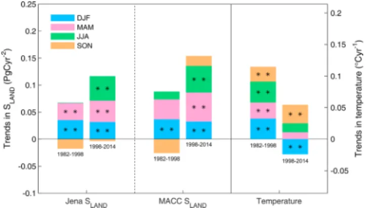
Figure 1 shows that the annual global 2 m air temperature warming rate decreased from 0.029°C yr 1 (p = 0.01) during the warming period (1982–1998) to 0.008°C yr 1 (p = 0.20) during the hiatus period (1998–2014), based on the CRU temperature data set. This is consistent with analyses that showed a warming hiatus starting in 1998 (Kosaka & Xie, 2013; Medhaug et al., 2017). Looking at the warming hiatus from a seasonal perspective, we found that a warming hiatus occurred only during March-April-May (MAM) and June-July-August (JJA). The respective temperature trends during MAM and JJA slowed by a factor of 2 from 0.026°C yr 1(p = 0.04) and 0.033°C yr 1(p< 0.01) during 1982–1998 to 0.011°C yr 1(p = 0.27) and 0.014°C yr 1(p = 0.11) during 1998–2014, respectively. By contrast, the global warming trends during September-October-November (SON) increased from 0.024°C yr 1(p = 0.09) during 1982–1998 to 0.030°C yr 1(p < 0.01) during the hiatus period. But the most significant change in the seasonal temperature trend occurred during December-January-February (DJF), going from a warming of 0.033°C yr 1(p = 0.08) to a cooling of 0.024°C yr 1(p = 0.09). We performed similar analyses using two other global temperature data sets (GHCN and GISS), the results of which are consistent with those derived from the CRU temperature data set (Figure S1 in the supporting information). Given that these temperature data sets are consistent with each other, we will mainly use the CRU in the following analyses.

3.2. Seasonal Land Carbon Flux Trend Changes

The annual global SLANDtrends increased from 0.050 Pg C yr 2(p = 0.27) during the warming period to

0.113 Pg C yr 2 (p < 0.01) during the hiatus period according to the Jena atmospheric inversion (Rödenbeck, 2005). The MACC inversion (Chevallier et al., 2010) also gives an accelerating SLANDduring the

warming hiatus (0.154 Pg C yr 2, p< 0.01) compared with the warming period (0.062 Pg C yr 2, p = 0.29) (Figure 1). If this acceleration of SLANDduring the hiatus period was due mainly to slower warming, the

changes in the seasonal SLANDtrends should match the seasonal temperature trend changes. We found a

sig-nificant increase in the SON warming trends, concurrent with the respective changes in the SLANDtrend going

from 0.018 Pg C yr 2 (p = 0.22, Jena) and 0.026 Pg C yr 2 (p = 0.13, MACC) during 1982–1998 to 0.004 Pg C yr 2(p = 0.78, Jena) and 0.019 Pg C yr 2(p = 0.18, MACC) during 1998–2014 (Figure 1). As an increase in respiration would be expected as a result of faster warming during SON during the hiatus period, the change in the SON SLANDtrend is unlikely to be the result of reduced respiration. Furthermore, Figure 1

shows that the most dramatic change in land temperature trends was mainly in DJF, as the temperature trend changed from warming (0.033°C yr 1, p = 0.08) to cooling ( 0.024°C yr 1, p = 0.09). During DJF, the trend in SLANDfrom inversions remained positive and to some extent unchanged (from 0.035 Pg C yr 2, p = 0.01, to

0.03 Pg C yr 2, p = 0.02 according to Jena and from 0.037 Pg C yr 2, p = 0.02, to 0.033 Pg C yr 2, p = 0.04 according to the MACC inversions). This also challenges the reducing respiration mechanism, since there was no faster decrease of the CO2source to the atmosphere in DJF during the hiatus period.

3.3. Changes in Seasonal Trends in Regional Land Carbon Flux and Temperature

The mismatch found between the changes in global temperature trends and global S_LANDtrends may be due to different and compensating regional effects (Jung et al., 2017). We thus analyzed the changes in seasonal SLANDfrom the warming period to the warming hiatus for 4 latitudinal bands and 11 TRANSCOM v3 regions

(Figure 2) (Baker et al., 2006). Generally, the two atmospheric inversions agree well with each other in terms of the seasonal S_LANDtrends in the boreal (>50°N), northern temperate (20–50°N), tropical (20°S–20°N), and southern latitudes (<20°S) regions during the warming period and warming hiatus (Figure S2). The most pro-nounced warming hiatus occurred in northern temperate latitudes (going from a warming of 0.032°C yr 1,

Figure 1. Trends in seasonal land carbon sink (SLAND) and seasonal

tempera-ture during 1982–1998 and 1998–2014 on a global scale. The trends in SLAND

were derived from two atmospheric CO2inversions (Jena s81_v3.8 and

MACC-II v11.2). Global temperature trends were derived from CRU TS v3.23. The two black asterisks indicate significant (p < 0.1) seasonal trends in SLAND

p = 0.04, to a cooling of 0.007°C yr 1, p = 0.37). The warming hiatus for this latitude band is caused mainly by a strong DJF cooling (from 0.060° C yr 1, p = 0.01, to 0.060°C yr 1, p = 0.01), while the other seasons do not show significant temperature trend changes. However, both atmospheric inversions suggest that the acceleration of SLANDoccurred mainly during JJA and SON.

The two atmospheric inversions agree well for seasonal S_LANDtrend changes in the three tropical regions (South American tropical, Northern Africa, and Tropical Asia). In the South American tropical region, the sea-sonal temperature trends remained constant during all seasons, while the corresponding seasea-sonal SLAND

trends all increased significantly. In Northern Africa, the temperature trends also remained constant during all seasons, but both atmospheric inversions suggest that the changes in seasonal SLANDtrends varied across

seasons. The seasonal SLANDtrends and temperature trends in these two tropical regions do not show a

nega-tive relationship between temperature and the SLANDtrends, implying that other factors are essential in

driv-ing the changes in the S_LANDtrend in the tropics. In comparison, the seasonal temperature trends decreased significantly in temperate South America and Southern Africa, while their seasonal SLANDtrends all decreased.

Table S1 shows the correlation coefficients between changes in SLANDtrends and changes in temperature

trends during each season across the 11 TRANSCOM regions. If the enhancement of land carbon sink is mainly due to warming hiatus-induced respiration decrease, there should be a negative correlation between changes in SLANDtrends and changes in temperature trends. However, their correlation coefficients are

nega-tive only during DJF (and nonsignificant) and positive during MAM, JJA, and SON. The positive correlation relationship between changes in S_LANDtrends and changes in temperature trends is relatively strong during JJA across the 11 TRANSCOM regions.

3.4. Analyzing the Response of Terrestrial Ecosystem Respiration to Temperature Change on a Seasonal or Annual Time Scale

Our results showed that the annual warming hiatus is composed of faster warming in SON, change from warming to cooling in DJF, and slower warming rates in MAM and JJA. This raises the question of how TER responds to changes in temperature trends from a seasonal perspective. According to the temperature dependency of TER (Davidson et al., 2006; Davidson & Janssens, 2006; Exbrayat et al., 2013; Luo et al., 2001; Raich et al., 2002), a change in temperature of the same magnitude can lead to different TER changes if

Figure 2. Trends in seasonal land carbon sink (SLAND) and temperature during 1982–1998 and 1998–2014 in the TRANSCOM regions. The trends in SLANDfor the

TRANSCOM regions were derived from two atmospheric CO2inversions (Jena s81_v3.8 and MACC-II v11.2). Temperature trends were derived from the CRU TS

v3.23. The two black dots indicate significant (p < 0.1) seasonal trends in SLANDor temperature.

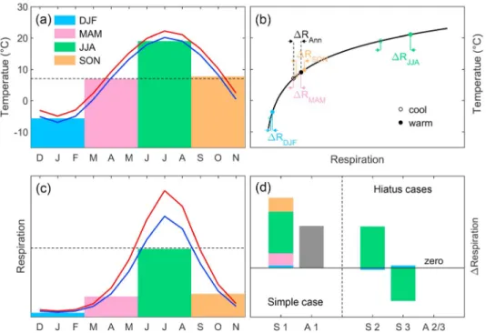
background temperature is different. Figure 3a shows the monthly and seasonal mean temperatures (background temperature) during 1982–2014 for the northern latitudes (>20°N), where the warming hiatus was most apparent. If we assume that the seasonal mean temperature increased similarly, the resulting changes in seasonal respiration would be divergent from the convex relationship between TER and temperature (Figure 3b). If we assume that carbon stocks and their quality do not change, the same temperature increment during all seasons should result in a small increase in TER during DJF, a medium increase during MAM and SON, and a significant increase during JJA (Figure 3c).

Figure 3d illustrates the resulting TER response under a uniform warming scenario (S1: same warming rate for all seasons) and two warming hiatus scenarios (S2: warming JJA and cooling DJF but no change in annual mean temperature and S3: cooling JJA and warming DJF, but no change in annual mean temperature) based on seasonal and annual analyses. For the uniform warming scenario S1, the increase in TER calculated at a seasonal time scale exceeds that calculated based on the changes in annual mean temperature because of interactions between background temperature and the temperature sensitivity of TER (Figure 3d, A1). For scenario S2, the increase in TER during JJA offsets the decrease in respiration during DJF, resulting in a net TER increase over a year. By contrast, scenario S3 would lead to a net decrease in annual TER. Under scenarios S2 and S3, TER would remain constant if calculated from annual temperature (Figure 3d, A2 and A3). Thus, investigating the response of soil respiration to temperature changes on annual time scale is not recom-mended, because this may mask asymmetrical seasonal temperature changes that are fundamental for ana-lyzing the respiration responses. Nevertheless, the seasonal variation of carbon available for decomposition is also important to consider in the real world.

Figure 3. Conceptual diagram of the response of respiration to temperature changes during each season. (a) Seasonal cycle of land surface temperature in the northern latitudes (>20°N) (blue line), where the warming hiatus was most apparent. The red line shows a simple warming case with an even and similar temperature increase during all seasons. The black dashed line shows the annual mean temperature. (b) Conceptual diagram of the response of respiration to tem-perature changes. (c) Asymmetrical response of respiration to temtem-perature changes during all seasons. (d) Response of respiration to temperature changes under different cases. S1 shows the seasonal changes in respiration with an even temperature increase during all seasons (simple case) estimated based on seasonal temperature, while A1 shows the annual changes in respiration under the simple case estimated based on the annual mean temperature. S2 shows the seasonal changes in respiration with increasing temperature during JJA and decreasing temperature (of the same mag-nitude as that during JJA) during DJF. S3 shows the seasonal changes in respiration with decreasing temperature during JJA and increasing temperature during DJF. Both scenarios result in no change in the annual mean temperature, that is, the hiatus cases. A2/A3 indicates no changes in annual respiration if estimated based on annual mean temperatures under the hiatus cases.

3.5. Changes in Seasonal Trends in GPP, TER, and NEP

We now use a range of land surface models to verify that ourfindings from observation-based NEP and conceptual model indicate that more complex processes caused the additional uptake of terrestrial carbon, rather than merely suppressed respiration. We used the TRENDY models to elucidate the roles of the main ecological processes in the SLANDtrend change during the warming hiatus (see section 2). The TRENDY

models generally reproduced the changes in global seasonal S_LANDtrends derived from the two atmospheric inversions (Figures S4 and S5). Figure 4 shows the changes in global seasonal GPP, TER, and NEP trends simu-lated by the TRENDY models forced by varying atmospheric CO2concentration and climatefields. The global

GPP trends did not change significantly between the two periods, from 0.361 ± 0.108 Pg C yr 2during 1982–1998 to 0.333 ± 0.147 Pg C yr 2during 1998–2014. The seasonal GPP trends decreased during SON (0.078 ± 0.035 to 0.058 ± 0.049 Pg C yr 2) and DJF (0.070 ± 0.025 to 0.038 ± 0.026 Pg C yr 2) but increased during MAM (0.085 ± 0.017 to 0.114 ± 0.033 Pg C yr 2) and did not change during JJA (0.129 ± 0.039 to 0.123 ± 0.050 Pg C yr 2). The decrease in the annual TER trend (0.310 ± 0.095 to 0.263 ± 0.124 Pg C yr 2) is slightly larger than that of annual GPP trends, resulting in a small increase in the annual NEP trend (0.051 ± 0.038 to 0.070 ± 0.052 Pg C yr 2). The decrease in the annual TER trend in the TRENDY models is mainly explained by a decrease in the TER trends during DJF (0.057 ± 0.018 to 0.029 ± 0.021 Pg C yr 2) and JJA (0.123 ± 0.040 to 0.093 ± 0.042 Pg C yr 2), although there is a weak increase in the TER trends during MAM (0.063 ± 0.020 to 0.075 ± 0.029 Pg C yr 2) and SON (0.068 ± 0.025 to 0.066 ± 0.041 Pg C yr 2). Generally, the changes in seasonal TER trends in the models match the changes in the seasonal temperature trends, except for those of MAM (Figure 1). During MAM, the increasing temperature trend slowed, while the TER trend increased slightly. This is likely due to the earlier start of the growing season that allows more time for MAM respiration and enhanced carbon uptake by the ecosystem as a result of CO2fertilization effects that

provides more carbohydrate for the respiration of plants (Forkel et al., 2016; Graven et al., 2013; Murray-Tortarolo et al., 2013; Sitch et al., 2015).

It should be noted that phenological responses and general growth dynamics could trigger possible memory between seasons (Vargas et al., 2010). We tested the legacy effects of seasonal GPP on subsequent seasonal NEP by calculating the partial correlation coefficients between the detrended time series of seasonal GPP and subsequent seasonal NEP in the TRANSCOM regions based on the TRENDY outputs. Our results showed that seasonal GPP significantly correlated with subsequent seasonal NEP in less than one-fourth cases (Table S2) and may not have significant impacts on our seasonal-based analyses because most of these cases are not accompanied with notable changes in seasonal NEP. Analyses based on model simulations under scenarios that control seasonal carbonfluxes and climatic variables may help further understanding of the memory processes between seasons.

To quantify the effects of the warming hiatus on the NEP trend changes, we forced the ORCHIDEE model by varying temperature only, keeping the other climatic variables and atmospheric CO2concentration constant.

The result showed that temperature change alone could not drive the global NEP trend from no change to a

Figure 4. Trends in seasonal gross primary production (GPP), terrestrial ecosystem respiration (TER), and net ecosystem production (NEP) simulated by the eight TRENDYv2 models (driven by varying CO2and climatefields) and seasonal

temperature during 1982–1998 and 1998–2014 on a global scale. The two black asterisks indicate significant (p < 0.1) seasonal trends in GPP, TER, NEP, or temperature. The error bar indicates the deviation between the models (one standard deviation).

significant increase (from 0.004 Pg C yr 2, p = 0.90 to 0.032 Pg C yr 2, p = 0.35). Note that the change in the global NEP trends simulated by the models forced by varying CO₂and climate (0.019 Pg C yr 2) is much smaller than that shown by the inversions (0.063 Pg C yr 2according to Jena and 0.100 Pg C yr 2according to MACC), suggesting that the processes missing from the model simulations are important. Indeed, when LUC was considered, the changes in global SLAND trends simulated by the TRENDY models increased

significantly by 0.115 Pg C yr 2from the warming to the hiatus periods. It implies that the decreased rates of deforestation and increased forest regrowth played an important role in the enhancement of SLAND, which

is encouraging for limiting global temperature rise to 2°C above preindustrial levels. We ran additional simulations with and without nitrogen deposition using CABLE, the difference between which was used to quantify the nitrogen deposition effects on changes in S_LANDtrends during the two periods. The results suggest that the effect of nitrogen deposition on changes in SLANDtrends is limited ( 0.010 Pg C yr 2), which

is consistent with a previous study suggesting that the changes in S_LAND due to nitrogen deposition is relatively small (Reay et al., 2008).

4. Conclusions

This study showed that both the seasonal and spatial patterns of changes in S_LANDtrends do not match those of changes in the temperature trends between the warming period (1982–1998) and warming hiatus (1998–2014). We also illustrated that changes in seasonal temperature during the hiatus are unlikely to cause a significant decrease in annual total respiration. Moreover, the TRENDY models driven by observed atmospheric CO2 concentration and climate fields suggest that warming hiatus cannot fully explain the

enhancement of SLAND. Instead, our study suggests that other mechanisms should be investigated to explain

the enhancement of SLANDduring the 2000s, which is important for understanding the

land-atmosphere-ocean carbon exchange in a new climate regime and projecting the future Earth system. Further study on the roles of other mechanisms may need comprehensive analyses based on multiple data sets because many complex problems should be resolved (Arneth et al., 2017; Le Quéré et al., 2016; Li et al., 2016). More research and new techniques, such as an increasing number of CO2satellites (Buchwitz et al., 2013) and the carbonyl

sulfide constraining framework (Campbell et al., 2017), combining with the Carbon Cycle Data Assimilation System (Kaminski et al., 2013; Rayner et al., 2005), are expected to help reconciling the contradictory explanations for the enhancement of S_LANDduring the recent decade.

References

Arneth, A., Sitch, S., Pongratz, J., Stocker, B. D., Ciais, P., Poulter, B.,… Zaehle, S. (2017). Historical carbon dioxide emissions caused by land-use changes are possibly larger than assumed. Nature Geoscience, 10(2), 79–84. https://doi.org/10.1038/ngeo2882

Baker, D. F., Law, R. M., Gurney, K. R., Rayner, P., Peylin, P., Denning, A. S.,… Zhu, Z. (2006). TransCom 3 inversion intercomparison: Impact of transport model errors on the interannual variability of regional CO2fluxes, 1988–2003. Global Biogeochemical Cycles, 20, GB1002. https://

doi.org/10.1029/2004GB002439

Ballantyne, A., Smith, W., Anderegg, W., Kauppi, P., Sarmiento, J., Tans, P.,… Running, S. (2017). Accelerating net terrestrial carbon uptake during the warming hiatus due to reduced respiration. Nature Climate Change, 7(2), 148–152. https://doi.org/10.1038/Nclimate3204 Ballantyne, A. P., Alden, C. B., Miller, J. B., Tans, P. P., & White, J. W. C. (2012). Increase in observed net carbon dioxide uptake by land and

oceans during the past 50 years. Nature, 488(7409), 70–72. https://doi.org/10.1038/nature11299

Bastos, A., Janssens, I. A., Gouveia, C. M., Trigo, R. M., Ciais, P., Chevallier, F.,… Running, S. W. (2016). European land CO2sink influenced by NAO

and East-Atlantic pattern coupling (Vol. 7, 10,315 pp.). https://doi.org/10.1038/ncomms10315

Buchwitz, M., Reuter, M., Bovensmann, H., Pillai, D., Heymann, J., Schneising, O.,… Löscher, A. (2013). Carbon monitoring satellite (CarbonSat): Assessment of atmospheric CO2and CH4retrieval errors by error parameterization. Atmospheric Measurement Techniques,

6(12), 3477–3500. https://doi.org/10.5194/amt-6-3477-2013

Campbell, J. E., Berry, J. A., Seibt, U., Smith, S. J., Montzka, S. A., Launois, T.,… Laine, M. (2017). Large historical growth in global terrestrial gross primary production. Nature, 544(7648), 84–87. https://doi.org/10.1038/nature22030

Chevallier, F., Ciais, P., Conway, T. J., Aalto, T., Anderson, B. E., Bousquet, P.,… Worthy, D. (2010). CO2surfacefluxes at grid point scale

estimated from a global 21 year reanalysis of atmospheric measurements. Journal of Geophysical Research, 115, D21307. https://doi.org/ 10.1029/2010JD013887

Ciais, P., Rayner, P., Chevallier, F., Bousquet, P., Logan, M., Peylin, P., & Ramonet, M. (2010). Atmospheric inversions for estimating CO2fluxes:

Methods and perspectives. Climatic Change, 103(1-2), 69–92. https://doi.org/10.1007/s10584-010-9909-3

Davidson, E. A., & Janssens, I. A. (2006). Temperature sensitivity of soil carbon decomposition and feedbacks to climate change. Nature, 440(7081), 165–173. https://doi.org/10.1038/nature04514

Davidson, E. A., Janssens, I. A., & Luo, Y. (2006). On the variability of respiration in terrestrial ecosystems: Moving beyond Q10. Global Change Biology, 12(2), 154–164. https://doi.org/10.1111/j.1365-2486.2005.01065.x

DeVries, T., Holzer, M., & Primeau, F. (2017). Recent increase in oceanic carbon uptake driven by weaker upper-ocean overturning. Nature, 542(7640), 215–218. https://doi.org/10.1038/nature21068

Exbrayat, J. F., Pitman, A. J., Zhang, Q., Abramowitz, G., & Wang, Y. P. (2013). Examining soil carbon uncertainty in a global model: Response of microbial decomposition to temperature, moisture and nutrient limitation. Biogeosciences, 10(11), 7095–7108. https://doi.org/10.5194/bg-10-7095-2013

Acknowledgments

Data used are available at http://www. cru.uea.ac.uk/data/ (CRUTS v3.23), https://www.ncdc.noaa.gov/temp-and-precip/ghcn-gridded-products/ (GHCN), https://data.giss.nasa.gov/gistemp/ (GISTEMP), https://ecocast.arc.nasa.gov/ data/pub/gimms/3g.v1/ (GIMMS NDVI3g v1), http://www.bgc-jena.mpg. de/CarboScope/?ID=s81_v3.8 (Jena s81_v3.8), and http://www.gmes-atmosphere.eu/ (MACC-II). This study was supported by the National Key R&D Program of China (2017YFA0604702), the National Natural Science Foundation of China (41530528, 41561134016 and 31621091), National Youth Top-notch Talent Support Program in China, and project funded by China Postdoctoral Science Foundation. We thank the TRENDY modeling group for providing the TRENDYv2 outputs.

Eyring, V., Bony, S., Meehl, G. A., Senior, C. A., Stevens, B., Stouffer, R. J., & Taylor, K. E. (2016). Overview of the Coupled Model Intercomparison Project Phase 6 (CMIP6) experimental design and organization. Geoscientific Model Development, 9(5), 1937–1958. https://doi.org/10.5194/ gmd-9-1937-2016

Forkel, M., Carvalhais, N., Rödenbeck, C., Keeling, R., Heimann, M., Thonicke, K.,… Reichstein, M. (2016). Enhanced seasonal CO2exchange

caused by amplified plant productivity in northern ecosystems. Science, 351(6274), 696–699. https://doi.org/10.1126/science.aac4971 Graven, H. D., Keeling, R. F., Piper, S. C., Patra, P. K., Stephens, B. B., Wofsy, S. C.,… Bent, J. D. (2013). Enhanced seasonal exchange of CO2by

northern ecosystems since 1960. Science, 341(6150), 1085–1089. https://doi.org/10.1126/science.1239207

Hansen, J., Ruedy, R., Sato, M., & Lo, K. (2010). Global surface temperature change. Reviews of Geophysics, 48, RG4004. https://doi.org/10.1029/ 2010RG000345

Harris, I., Jones, P. D., Osborn, T. J., & Lister, D. H. (2014). Updated high-resolution grids of monthly climatic observations—The CRU TS3.10 dataset. International Journal of Climatology, 34(3), 623–642. https://doi.org/10.1002/joc.3711

Intergovernmental Panel on Climate Change (2013). Climate change 2013: The physical science basis. Contribution of Working Group I to the Fifth Assessment Report of the Intergovernmental Panel on Climate Change (1535 pp.). Cambridge, UK and New York: Cambridge University Press. Jones, P. D., & Moberg, A. (2003). Hemispheric and large-scale surface air temperature variations: An extensive revision and an update to

2001. Journal of Climate, 16(2), 206–223. https://doi.org/10.1175/1520-0442(2003)016%3C0206:halssa%3E2.0.co;2

Jung, M., Reichstein, M., Schwalm, C. R., Huntingford, C., Sitch, S., Ahlström, A.,… Zeng, N. (2017). Compensatory water effects link yearly global land CO2sink changes to temperature. Nature, 541(7638), 516–520. https://doi.org/10.1038/nature20780

Kaminski, T., Knorr, W., Schürmann, G., Scholze, M., Rayner, P. J., Zaehle, S.,… Ziehn, T. (2013). The BETHY/JSBACH carbon cycle data assimilation system: Experiences and challenges. Journal of Geophysical Research: Biogeosciences, 118, 1414–1426. https://doi.org/10.1002/jgrg.20118 Keeling, C. D., & Whorf, T. P. (2005). Atmospheric CO2records from sites in the SIO air sampling network. In Trends: A compendium of data on

global change. Oak Ridge: Carbon Dioxide Information Analysis Center, Oak Ridge National Laboratory, US Department of Energy. Retrieved from http://cdiac.esd.ornl.gov/trends/co2/sio-mlo.htm

Keenan, T. F., Prentice, I. C., Canadell, J. G., Williams, C. A., Wang, H., Raupach, M., & Collatz, G. J. (2016). Recent pause in the growth rate of atmospheric CO2due to enhanced terrestrial carbon uptake. Nature Communications, 7, 13,428. https://doi.org/10.1038/ncomms13428

Kosaka, Y., & Xie, S.-P. (2013). Recent global-warming hiatus tied to equatorial Pacific surface cooling. Nature, 501(7467), 403–407. https://doi. org/10.1038/nature12534

Le Quéré, C., Andrew, R. M., Canadell, J. G., Sitch, S., Korsbakken, J. I., Peters, G. P.,… Zaehle, S. (2016). Global carbon budget 2016. Earth System Science Data, 8(2), 605–649. https://doi.org/10.5194/essd-8-605-2016

Le Quéré, C., Peters, G. P., Andres, R. J., Andrew, R. M., Boden, T., Ciais, P.,… Yue, C. (2013). Global carbon budget 2013. Earth System Science Data Discussions, 6(2), 689–760. https://doi.org/10.5194/essdd-6-689-2013

Li, W., Ciais, P., Wang, Y., Peng, S., Broquet, G., Ballantyne, A. P.,… Pongratz, J. (2016). Reducing uncertainties in decadal variability of the global carbon budget with multiple datasets. Proceedings of the National Academy of Sciences of the United States of America, 113(46), 13,104–13,108. https://doi.org/10.1073/pnas.1603956113

Luo, Y., Wan, S., Hui, D., & Wallace, L. L. (2001). Acclimatization of soil respiration to warming in a tall grass prairie. Nature, 413(6856), 622–625. https://doi.org/10.1038/35098065

Medhaug, I., Stolpe, M. B., Fischer, E. M., & Knutti, R. (2017). Reconciling controversies about the“global warming hiatus”. Nature, 545(7652), 41–47. https://doi.org/10.1038/nature22315

Mikaloff Fletcher, S. E., Gruber, N., Jacobson, A. R., Doney, S. C., Dutkiewicz, S., Gerber, M.,… Sarmiento, J. L. (2006). Inverse estimates of anthropogenic CO2uptake, transport, and storage by the ocean. Global Biogeochemical Cycles, 20, GB2002. https://doi.org/10.1029/

2005GB002530

Murray-Tortarolo, G., Anav, A., Sitch, S., Zhu, Z., Poulter, B., Zaehle, S.,… Zeng, N. (2013). Evaluation of land surface models in reproducing satellite-derived LAI over the high-latitude Northern Hemisphere. Part I: Uncoupled DGVMs. Remote Sensing, 5(10), 4819.

New, M., Hulme, M., & Jones, P. (2000). Representing twentieth-century space-time climate variability. Part II: Development of 1901–96 monthly grids of terrestrial surface climate. Journal of Climate, 13(13), 2217–2238. https://doi.org/10.1175/1520-0442(2000)013%3C2217: RTCSTC%3E2.0.CO;2

Peterson, T. C., & Vose, R. S. (1997). An overview of the global historical climatology network temperature database. Bulletin of the American Meteorological Society, 78(12), 2837–2849. https://doi.org/10.1175/1520-0477(1997)078%3C2837:aootgh%3E2.0.co;2

Peylin, P., Law, R. M., Gurney, K. R., Chevallier, F., Jacobson, A. R., Maki, T.,… Zhang, X. (2013). Global atmospheric carbon budget: Results from an ensemble of atmospheric CO2inversions. Biogeosciences, 10(10), 6699–6720. https://doi.org/10.5194/bg-10-6699-2013

Pinzon, J., & Tucker, C. (2014). A non-stationary 1981–2012 AVHRR NDVI3g time series. Remote Sensing, 6(8), 6929–6960. https://doi.org/ 10.3390/rs6086929

Pongratz, J., Reick, C. H., Houghton, R. A., & House, J. I. (2014). Terminology as a key uncertainty in net land use and land cover change carbon flux estimates. Earth System Dynamics, 5(1), 177–195. https://doi.org/10.5194/esd-5-177-2014

Poulter, B., Frank, D., Ciais, P., Myneni, R. B., Andela, N., Bi, J.,… van der Werf, G. R. (2014). Contribution of semi-arid ecosystems to interannual variability of the global carbon cycle. Nature, 509(7502), 600–603. https://doi.org/10.1038/nature13376

Raich, J. W., Potter, C. S., & Bhagawati, D. (2002). Interannual variability in global soil respiration, 1980–94. Global Change Biology, 8(8), 800–812. https://doi.org/10.1046/j.1365-2486.2002.00511.x

Rayner, P. J., Scholze, M., Knorr, W., Kaminski, T., Giering, R., & Widmann, H. (2005). Two decades of terrestrial carbonfluxes from a carbon cycle data assimilation system (CCDAS). Global Biogeochemical Cycles, 19, GB2026. https://doi.org/10.1029/2004GB002254

Reay, D. S., Dentener, F., Smith, P., Grace, J., & Feely, R. A. (2008). Global nitrogen deposition and carbon sinks. Nature Geoscience, 1(7), 430–437. https://doi.org/10.1038/ngeo230

Rödenbeck, C. (2005). Estimating CO2sources and sinks from atmospheric mixing ratio measurements using a global inversion of

atmo-spheric transport (Technical Report 6). Jena: Max Planck Institute for Biogeochemistry.

Schimel, D., Stephens, B. B., & Fisher, J. B. (2015). Effect of increasing CO2on the terrestrial carbon cycle. Proceedings of the National Academy

of Sciences, 112(2), 436–441. https://doi.org/10.1073/pnas.1407302112

Sitch, S., Friedlingstein, P., Gruber, N., Jones, S. D., Murray-Tortarolo, G., Ahlström, A.,… Myneni, R. (2015). Recent trends and drivers of regional sources and sinks of carbon dioxide. Biogeosciences, 12(3), 653–679. https://doi.org/10.5194/bg-12-653-2015

Takahashi, T., Sutherland, S. C., Wanninkhof, R., Sweeney, C., Feely, R. A., Chipman, D. W.,… de Baar, H. J. W. (2009). Climatological mean and decadal change in surface ocean pCO2, and net sea–air CO2flux over the global oceans. Deep Sea Research Part II: Topical Studies in

Oceanography, 56(8), 554–577. https://doi.org/10.1016/j.dsr2.2008.12.009

Vargas, R., Baldocchi, D. D., Allen, M. F., Bahn, M., Black, T. A., Collins, S. L.,… Tang, J. (2010). Looking deeper into the soil: Biophysical controls and seasonal lags of soil CO2production and efflux. Ecological Applications, 20(6), 1569–1582. https://doi.org/10.1890/09-0693.1