HAL Id: hal-02163454
https://hal.archives-ouvertes.fr/hal-02163454v2
Submitted on 11 Mar 2020
HAL is a multi-disciplinary open access
archive for the deposit and dissemination of
sci-entific research documents, whether they are
pub-lished or not. The documents may come from
teaching and research institutions in France or
abroad, or from public or private research centers.
L’archive ouverte pluridisciplinaire HAL, est
destinée au dépôt et à la diffusion de documents
scientifiques de niveau recherche, publiés ou non,
émanant des établissements d’enseignement et de
recherche français ou étrangers, des laboratoires
publics ou privés.
SHALLOW WATER EQUATIONS
Raphaèle Herbin, Jean-Claude Latché, Youssouf Nasseri, Nicolas Therme
To cite this version:
Raphaèle Herbin, Jean-Claude Latché, Youssouf Nasseri, Nicolas Therme. A DECOUPLED
STAG-GERED SCHEME FOR THE SHALLOW WATER EQUATIONS. Fifteenth International Conference
Zaragoza-Pau on Mathematics and its Applications, Sep 2018, Jaca, Spain. �hal-02163454v2�
A
DECOUPLED STAGGERED SCHEME
FOR THE SHALLOW WATER EQUATIONS
Raphaèle Herbin, Jean-Claude Latché, Youssouf Nasseri and
Nicolas Therme
Abstract. We present a first order scheme based on a staggered grid for the shallow water equations with topography in two space dimensions, which enjoys several properties: positivity of the water height, preservation of constant states, and weak consistency with the equations of the problem and with the associated entropy inequality.
Keywords: Shallow water, finite volumes, staggered grid. AMS classification: 65M08,76B99.
§1. Introduction
The shallow water equations form a hyperbolic system of two conservation equations (mass and momentum) which are obtained when modelling a flow whose vertical height is consid-ered small with respect to the plane scale. The solution of such a system may develop shocks, so that the finite volume method is usually preferred for numerical simulations. Two main approaches are found: one is the colocated approach which is usually based on some approx-imate Riemann solver, see e.g. [3] and references therein; the other one is based on a stag-gered arrangement of the unknowns on the grid. Indeed, stagstag-gered schemes have been used for some time in the hydraulic and ocean engineering community, see e.g. [1, 2, 12]. They have been recently analysed in the case of one space dimension [5, 8], following the works on the related barotropic Euler equations, see [11] and references therein. In the present work, we obtain a discrete local entropy inequality; furthermore, we extend the consistency analysis of the scheme to the case of two space dimensions, and we weaken the assumptions on the es-timates, namely we no longer require a bound on the BV norm of the approximate solutions, at least for the weak formulation (the passage to the limit in the entropy still necessitates a time BV boundedness).
Let Ω be an open bounded domain of R2 and let T > 0. We consider the shallow water
equations with topography over the space and time domain Ω × (0, T):
∂th + div(hu) = 0 in Ω × (0, T), (1a) ∂t(hu) + div(hu ⊗ u) + ∇p + gh∇z = 0 in Ω × (0, T), (1b) p = 1 2gh2 in Ω × (0, T), (1c) u · n = 0 on ∂Ω × (0, T), (1d) h(x, 0) = h0, u(x, 0) = u0 in Ω. (1e)
where t stands for the time, g is the standard gravity constant and z the (given) topography, which is supposed to be regular in this paper. These equations solve the water height h and the velocityu.
Let us recall that if (h,u) is a regular solution of (1), the following elastic potential energy balance and kinetic energy balance is obtained by manipulations on the mass and momentum equations: ∂t(1 2gh2) + div( 1 2gh2u) + 1 2gh2divu = 0 (2) ∂t(1 2h|u|2) + div( 1 2h|u|2u) + u · ∇p + ghu · ∇z = 0. (3) Summing these equations, we obtain en entropy equality of the form ∂tη +divΦ = 0, where
the entropy-entropy flux pair (η, Φ) is given by: η = 1 2h|u|2+ 1 2gh2+ ghz and Φ = (η + 1 2gh2)u. (4) For non regular functions the above manipulations are no longer valid, and the entropy in-equality ∂tη +divΦ ≤ 0 is satisfied in a distributional sense.
In this paper, we build a decoupled scheme, involving only explicit steps; the resulting ap-proximate solutions are shown to satisfy some discrete equivalent of (2) and (3); furthermore, under some convergence and boundedness assumptions, the approximate solutions are shown in Section 5 to converge to a weak solution of (1) and to satisfy a weak entropy inequality.
§2. Mesh and space discretizations
Let Ω be a connected subset of R2 consisting in a union of rectangles whose edges are
as-sumed to be orthogonal to the canonical basis vectors, denoted by (e(1),e(2)).
Definition 1 (MAC grid). A discretization (M, E) of Ω with a staggered rectangular grid (or MAC grid), is defined by:
– A primal grid M which consists in a conforming structured partition of Ω in rectan-gles, possibly non uniform. A generic cell of this grid is denoted by K, and its mass center byxK. The scalar unknowns (water height and pressure) are associated to this
mesh.
– The set of all edges of the mesh E, with E = Eint∪ Eext, where Eint(resp. Eext) are
the edges of E that lie in the interior (resp. on the boundary) of the domain. The set of edges that are orthogonal toe(i)is denoted by E(i), for i = 1, 2. We then have
E(i) =E(i)
int∪ E(i)ext, where E(i)int (resp. E(i)ext) are the edges of E(i)that lie in the interior
(resp. on the boundary) of the domain.
For σ ∈ Eint, we write σ = K|L if σ = ∂K ∩ ∂L. A dual cell Dσassociated to an edge
σ∈ E is defined as follows:
- if σ = K|L ∈ Eint then Dσ = DK,σ∪ DL,σ, where DK,σ(resp. DL,σ) is the
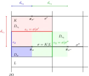
D!1 D!3 K L σ = K|L Dσ σ′′ × × × xσ′ xσ xσ′′ "2 "3= σ|σ′′ σ′ "1= σ|σ′ ∂Ω d!3 d!2 d!1 1
Figure 1: Notations for control volumes and dual cells (in two space dimensions, for the second component of the velocity).
- if σ ∈ Eextis adjacent to the cell K, then Dσ=DK,σ.
For each dimension i = 1, 2, the domain Ω is partitioned in dual cells: Ω = ∪σ∈E(i)Dσ,
i = 1, 2; the ith partition is refered to as the ith dual mesh; it is associated to the ith
velocity component, in a sense which is clarified below. The set of the edges of the ith
dual mesh is denoted by E(i)(note that these edges may be orthogonal to any vector
of the basis of R2and not onlye(i)) and is decomposed into the internal and boundary
edges: E(i) = E(i)
int∪ E(i)ext. The dual edge separating two duals cells Dσ and Dσ′ is
denoted by = σ|σ′. We denote by D
the dual cell associated to a dual edge ∈ E
defined as follows:
- if = σ|σ′ ∈ Eint then D
= Dσ, ∪ Dσ′,, where Dσ, (resp. Dσ′,) is the
half-part of Dσ(resp. Dσ′) adjacent to (see Fig. 1);
- if ∈ Eextis adjacent to the cell Dσ, then D=Dσ,.
In order to define the scheme, we need some additional notations. The set of edges of a primal cell K and of a dual cell Dσare denoted by E(K) and E(Dσ) respectively. For σ ∈ E,
we denote byxσthe mass center of σ. The vectornK,σstands for the unit normal vector to σ
outward K. In some cases, we need to specify the orientation of various geometrical entities with respect to the axis:
- a primal cell K will be denoted K = [−−−→σσ′] if σ, σ′∈ E(i)(K) for some i = 1, 2 are such
that (xσ′− xσ) · e(i)>0;
- we write σ = −−→K|L if σ ∈ E(i), σ = K|L and −−−−→x
KxL· e(i)>0 for some i = 1, 2;
- the dual edge separating Dσand Dσ′is written = −−−→σ|σ′if −−−−→xσxσ′· e(i)>0 for some
The size δMof the mesh and its regularity ηMare defined by:
δM=max
K∈Mdiam(K), and ηM=max
|σ|
|σ′|, σ∈ E(i), σ′∈ E( j), i, j = 1, 2, i j
, (5)
where | · | stands for the one (or two) dimensional measure of a subset of R (or R2).
The discrete velocity unknowns are associated to the dual cells and denoted by (ui,σ)σ∈E(i),
i = 1, 2, while the scalar unknowns (discrete water height and pressure) are associated to the primal cells and are denoted respectively by (hK)K∈Mand (pK)K∈M. The scalar unknown
space LMis defined as the set of piecewise constant functions over each grid cell K of M,
and the discrete ithvelocity space H
E(i) as the set of piecewise constant functions over each of
the grid cells Dσ, σ∈ E(i). As in the continuous case, the Dirichlet boundary conditions are
taken into account by defining the subspaces HE(i),0⊂ HE(i), i = 1, 2 as follows
HE(i),0 =
ui∈ HE(i), ui(x) = 0, ∀x ∈ Dσ, σ∈ E(i)ext
.
We then set HE,0 = HE(1),0× HE(2),0. Defining the characteristic function 11A of any subset
A ⊂ Ω by 11A(x) = 1 if x ∈ A and 11A(x) = 0 otherwise, the functions u = (u1,u2) ∈ HE,0,
may then be written:
ui(x) =
σ∈E(i)
ui,σ11Dσ(x), i = 1, 2. (6)
Foru ∈ HE,0, let ui = |ui,σ− ui,σ′|, for = σ|σ′ ∈ E(i)int,i = 1, 2. In the same way
the functions h ∈ LM are defined by h(x) = K∈MhK11K(x) and the notation σ refers to
hσ=|hK− hL|, for σ = K|L ∈ Eint(K).
§3. A decoupled explicit scheme
Description of the scheme Let us consider a uniform discretisation 0 = t0<t1<· · · < tN=
T of the time interval (0, T), and let δt = tn+1− tnfor n = 0, 1, · · · , N − 1 be the (constant)
time step. The discrete velocityu and water height h unknowns are defined by:
u(x, t) =N−1 n=0 un+1(x)11 [tn,tn+1)(t), withun+1∈ HE,0, h(x, t) =N−1 n=0 hn+1(x)11 [tn,tn+1)(t), with hn+1∈ LM,
where 11[tn,tn+1) is the characteristic function of the interval [tn,tn+1) and the space functions
unand hntake the form defined in the previous section. We propose the following decoupled
defined below.
Initialisation: u0=P
Eu0,h0=PMh0, p0= 12g(h0)2. (7a)
Iteration n, 0 ≤ n ≤ N − 1 : solve for un+1∈ H
E,0,hn+1∈ LMand pn+1∈ LM:
ðthn+1+divM(hnun) = 0, (7b)
pn+1= 1
2g(hn+1)2, (7c) ðt(hu)n+1+CE(hnun)un+∇Epn+1+ gIEhn+1∇Ez = 0, (7d) Projection operators - The operators PEand PMused in the initialisation step are defined
by PE=(PE(i))i=1,··· ,dwith
PE(i) : L1(Ω) −→ HE(i),0
v −→ PE(i)v =
σ∈E(i)int
vσ11Dσwith vσ= 1 |Dσ| Dσ v(x) dx, for σ ∈ E(i) int. (8) For q ∈ L2(Ω), P Mq ∈ LMis defined by: PMq = K∈M qK11Kwith qK = 1 |K| Kq(x) dx for K ∈ M. (9)
Discrete time derivative - The symbol ðt denotes the discrete time derivative for both
water height and momentum: ðthn+1=
K∈M
ðthn+1K 11K, ðthn+1K =
1
δt(hn+1K − hnK), and ðt(hu)n+1=(ðt(hu1)n+1, ðt(hu2)n+1)
with ðt(hui)n+1=
σ∈E(i)
ðt(hui)n+1σ 11Dσ, and ðt(hui)
n+1 σ = 1 δt(hn+1Dσu n+1 i,σ − hnDσu n i,σ), i = 1, 2,
where hDσ is the discrete water height in the dual cell, which is computed from the primal
unknowns (hn
K)n∈N,K∈Mand defined so as to satisfy a discrete mass balance, see below.
Discrete divergence and gradient operators - The discrete divergence operator divM is
de-fined by:
divM: HE,0−→ LM,0
u −→ divM(hu) =
K∈M
divK(hu)11K, with divK(hu) = 1
|K|
σ∈E(K)
FK,σ, (10)
where FK,σ is the (conservative) numerical mass flux, defined by FK,σ = |σ| hσuK,σ with
uK,σ=ui,σnK,σ· e(i)for σ ∈ E(i)int, i = 1, 2, while hσis approximated by the first order upwind
The discrete gradient operator applies to the pressure and the topography and is defined by: ∇E: LM−→ HE,0 p −→ ∇Ep, with for i = 1, 2: (∇Ep)i=
σ∈E(i)int
ðσp11Dσ with for σ = −−→K|L, ðσp = |
σ|
|Dσ|(pL− pK). (11)
The above defined discrete divergence and gradient operators satisfy the following div-grad duality relationship [7, Lemma 2.5]:
for p ∈ LM,u ∈ HE,0, Ω p divM(u) dx + Ω∇Ep · u dx = 0.
Discrete convection operator – The discrete nonlinear convection operator CE(hu) is
linked to the discrete divergence operator on the dual mesh by the relation CE(hu)u =
divE(hu ⊗ u), where the full discrete convection operator CE(hu) is defined by:
CE(hu) u = CE(1)(hu) u1,CE(2)(hu) u2,
and the i-th component CE(i)(hu) of the convection operator is defined by:
CE(i)(hu) : HE(i),0−→ HE(i),0
ui−→ CE(i)(hu) ui=
σ∈E(i)int
divE(i)(huiu) 11Dσ,
with divE(i)(huiu) = 1
|Dσ|
∈E(Dσ)
Fσ,ui,,
(12)
where for = σ|σ′, ui,is the upwind choice between u
σand uσ′with respect to the sign of
Fσ,. The quantity Fσ,is the numerical mass flux through outward Dσ; it must be chosen
carefully to ensure some stability properties of the scheme as in [7, 11]. Indeed we recall that in order to derive a discrete kinetic energy balance (Lemma 3 below), it is necessary that a discrete equation of the mass balance holds in the dual mesh, namely:
|Dσ| δt (hn+1Dσ − h n Dσ) + divE(h nun) = 0, with |D σ| divE(hnun) = ∈E(Dσ) Fn σ,. (13)
The water height hDσand the flux Fσ,are computed from the primal unknowns and fluxes so
as to satisfy this latter relation thanks to the discrete mass balance on the primal mesh (7b). For σ = K|L ∈ Eint, the water height hDσ is defined as a weighted average between hK and
hL:
|Dσ| hDσ =|DK,σ| hK+|DL,σ| hL, (14)
where Dσ, DK,σand DL,σare defined in Definition 1. The numerical flux Fσ, on the internal
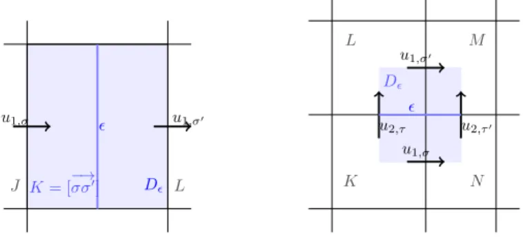
D! u1,σ ! u1,σ′ K = [−→σσ′] J L D! K L M N u1,σ u2,τ u1,σ′ u2,τ′ ! 1
Figure 2: Notations for the definition of the momentum flux on the dual mesh for the first component of the velocity- left: first case - right: second case.
- First case – The vectore(i)is normal to , and is included in a primal cell K, with
K = [−−−→σσ′] (see Definition 1 and Figure 2 on the left for i = 1). Then for a dual edge ∈ E(i)such that = −−−→σ|σ′, the flux Fσ,through the edge is given by:
Fσ,= 1 2(FK,σ′− FK,σ) = 1 2|| (hσui,σ+hσ′ui,σ′), (15) since |σ| = |σ′| = ||.
- Second case – The vectore(i)is tangent to , and is the union of the halves of two
primal edges τ and τ′ such that τ = −−→K|L, τ ∈ E(K) and τ′ = −−−→N|M ∈ E(N) (see
Definition 1 and Figure 2 on the right for i = 1). Let j ∈ {1, 2}, j i: the numerical flux through is then given by:
Fσ, = 1
2 (FKτ+FLτ′) = 1
2 (|τ| hτuj,τ+|τ′| hτ′uj,τ′). (16)
Note that the numerical momentum flux on a dual edge is conservative. It is easy to check that the unknowns hn
Dσ and F
n
σ,thus defined satisfy the discrete dual mass balance (13).
Discrete water height on the dual mesh, for the topography term – In equation (7d) the interpolation operatorIEis defined as the mean value of the water height:
IEh = σ∈Eint hσ,c11Dσ with hσ,c= 1 2(hK+hL) for σ = K|L ∈ Eint,
hKfor σ ∈ Eext∩ E(K).
(17) This choice is important to preserve steady states, see Lemma 2.
§4. Properties of the scheme
The scheme (7) enjoys some interesting properties, which we now state. First of all, thanks to the upwind choice for hnin (1a), the positivity of the water height is preserved under a CFL
Lemma 1 (Positivity of the water height). Let n ∈ 0, N −1, let (hn
K,uni,σ)K∈M, σ∈E(i)be given
and such that hn
K ≥ 0, for all K ∈ M, and let hn+1K be computed by (7b). Then hn+1K ≥ 0, for
all K ∈ M under the following CFL condition, ∀K ∈ M, δt ≤ |K|
σ∈E(K)
|σ| |unK,σ|
. (18)
Second, thanks to the choice (17) for the reconstruction of the water height, the "lake at rest" steady state is preserved by the scheme.
Lemma 2 (Steady state "lake at rest"). Let n ∈ 0, N − 1, C ∈ R+; let un+1 ∈ HE,0 and
hn+1 ∈ L
Mbe a solution to (7b)-(7d) withun =0 and hn+z = C, where C is a given real
number. Thenun+1=0 and hn+1+z = C.
As a consequence of the careful discretisation of the convection term, the scheme satisfies a discrete kinetic energy balance, as stated in the following lemma. The proof of this result is an easy adaptation of [10, Lemma 3.2].
Lemma 3 (Discrete kinetic energy balance). A solution to the scheme (7) satisfies the fol-lowing equality, for i = 1, 2, σ ∈ E(i)and 0 ≤ n ≤ N − 1:
1 2 δt(hn+1Dσ(u n+1 i,σ)2− hnDσ(u n i,σ)2) + 1 2 |Dσ| ∈E(i)(Dσ) Fn σ,(uni,)2
+un+1i,σðσpn+1+ ghσ,cn+1un+1i,σðσz = −Rn+1i,σ, (19)
with Rn+1
i,σ ≥ 0 under the CFL like restriction:
∀σ ∈ E(i), δt ≤ |Dσ| hn+1Dσ ∈E(Dσ) (Fn σ,)− . (20)
The scheme also satisfies the following potential energy balance [10, Lemma 3.3]. Lemma 4 (Discrete elastic potential balance). Let, for K ∈ M and 0 ≤ n ≤ N the potential energy be defined by (Ep)nK = 12g(hnK)2. A solution to the scheme (7) satisfies the following
equality, for K ∈ M and 0 ≤ n ≤ N − 1:
(ðtEp)n+1K +divK(Enpun) + pnKdivKun=−Rn+1K , (21) with Rn+1 K ≥|K|1 g σ∈E(K) |σ| unK,σhnσ(hn+1K − hnK). (22)
Note that the right-hand side of Equation (22) may be negative, and thus also the quan-tities Rn+1
K . This is specific to explicit schemes (for implicit or pressure-correction schemes,
However, combining the two previous lemmas allows to prove that convergent sequences of solutions to the scheme satisfy an entropy inequality, as depicted in the next section. To this purpose, we will pass to the limit in a discrete entropy balance which is built as follows. Let K ∈ M and let us denote by (Ek)nK the following quantity, which may be seen as a kinetic
energy associated to K: (Ek)nK = 1 4 |K| 2 i=1 σ∈E(K)∩E(i) |Dσ| hnDσ(uni,σ)2.
Then, for σ0∈ E(K), we define a kinetic energy flux, which we denote by GnK,σ0, as follows.
Let us suppose, for instance, that σ0 ∈ E(1). We denote by the face of Dσ0 parallel to σ0
and included in K and by ′the opposite face of Dσ
0. In addition, σ0 is the union of two
half-faces of the dual mesh associated to the second component of the velocity, which we denote by τ and τ′, and we denote by σ and σ′the two faces of K belonging to E(2)such that
τ∈ E(Dσ) and τ′∈ E(Dσ′). We then set:
Gn K,σ0= 1 4 −Fn σ0,(u n 1,)2+Fσn0,′(u n 1,′)2+Fnσ,τ(un2,τ)2+Fnσ,τ′(un2,τ′)2
Multiplying the kinetic energy balance equation (19) associated to each face σ of K by 1 2|Dσ|
and summing the four obtained relations with Equation (21) multiplied by |K|, we get
(ðtEk)n+1K +(ðtEp)n+1K + σ∈E(K) Gn K,σ+12ghnσFnK,σ+ σ∈E(K) σ=K|L |σ|pnKunK,σ + σ∈E(K) σ=K|L |σ| 12 (pn+1 L − pn+1K ) un+1K,σ+ σ∈E(K) σ=K|L |σ| 14g(hn+1 K +hn+1L ) (zL− zK) un+1K,σ=−TKn+1, where Tn+1
K collects the residual terms in (19) and (21), and thus TKn+1≥ Rn+1K . We now remark
that, thanks to the discrete mass balance equation and the fact that the topography does not depend on time, 1 2 σ∈E(K) Fn K,σ(zL− zK) = |K| δt (hn+1K zK− hnKzK) +1 2 σ∈E(K), σ=K|L Fn K,σ(zK+zL),
and we finally obtain the following discrete entropy balance:
(ðtEk)n+1K +(ðtEp)n+1K + gzK(ðth)n+1K + σ∈E(K) Gn K,σ+12ghnσFnK,σ+12FnK,σ(zK+zL) + σ∈E(K) σ=K|L |σ| 12 (pn K+pnL) unK,σ=−(Re)n+1K , (23)
with (Re)n+1K ≥ TKn+1+ g σ∈E(K) 1 2F n K,σ− 1 4|σ| (hn+1K +hLn+1) un+1K,σ (zL− zK) + σ∈E(K), σ=K|L |σ|12 (pn+1 K un+1K,σ− pnKunK,σ+pn+1L un+1L,σ− pnLunL,σ). (24)
Note that the above remainder term Recannot be proven to be non negative ; however, the
relation (24) allows to obtain a weak entropy consistency property when passing to the limit, as stated in the next section.
§5. Consistency analysis
The objective of this section is to show that the schemes are consistent in the Lax-Wendroff sense, namely that if a sequence of solutions is controlled in suitable norms and converges to a limit, this latter necessarily satisfies a weak formulation of the continuous problem.
A weak solution to the continuous problem satisfies, for any ϕ ∈ C∞
cΩ× [0, T) (ϕ ∈ C∞ cΩ× [0, T)2): T 0 Ω h ∂tϕ +h u · ∇ϕ dx dt + Ω h0(x) ϕ(x, 0) dx = 0, (25a) − T 0 Ω hu · ∂tϕ +(hu ⊗ u) : ϕ +1 2 gh2div(ϕ) + g h ∇(z)ϕ dx dt (25b) − Ω h0(x) u0(x) · ϕ(x, 0) dx = 0.
This system is supplemented with a weak entropy inequality, for any nonnegative test func-tions ϕ ∈ C∞ cΩ× [0, T), R+ : − T 0 Ω η ∂tϕ + Φ· ∇ϕ dx dt − Ω η0(x) ϕ(x, 0) dx ≤ 0, (26) with η and Φ defined by (4).
Before stating the global weak consistency of the scheme (7), some definitions and esti-mate assumptions are needed.
Let (M(m),E(m))
m∈Nbe a sequence of meshes in the sense of Definition 1 and let (h(m)
u(m))
m∈Nbe the associated sequence of solutions of the scheme (7)).
Assumed estimates - We need also some a priori estimates on the sequence of discrete solutions (h(m), u(m))
m∈Nin order to prove the consistency result we are seeking. First of all
we assume that h(m) > 0, ∀m ∈ N which can be obtained under the CFL condition (18).
– The water height h(m)and its inverse are uniformly bounded in L∞(Ω×(0, T)), i.e.there
exists some constants C, C′∈ R∗
+such that for m ∈ N and 0 ≤ n < N(m):
1/C < (h(m))n
K ≤ C, 1/C′<1/(h(m))nK≤ C′ ∀K ∈ M(m) (27)
– The velocityu(m)is also uniformly bounded in L∞(Ω × (0, T))2:
|(u(m))n
σ| ≤ C, ∀σ ∈ E(m). (28)
Finally, the weak consistency to the entropy inequality is only proved under additional as-sumptions. First we need the following condition on the space and time steps, which is stronger than a CFL condition:
δt(m)
δM(m) → 0 as m → +∞ (29)
Second, the L1(Ω, BV) norm of the height is required to be bounded, i.e. there exists one
constant C such that, for m ∈ N,
N−1 n=0 K∈M |K| |(h(m))n+1 K − (h(m))nK| ≤ C. (30)
We are now in position to state the following consistency result. Theorem 5 (Weak consistency of the scheme). Let (M(m),E(m))
m∈Nbe a sequence of meshes
such that δt(m) and δ
M(m) → 0 as m → +∞ ; assume that there exists η > 0 such that
ηM(m) ≤ η for any m ∈ N (with ηM(m) defined by (5)); assume moreover that (27) and (28)
hold. Let (h(m),u(m))
m∈Nbe a sequence of solutions to the scheme (7) converging to (¯h, ¯u) in
L1(Ω ×(0, T))× L1(Ω ×(0, T))2. Then (¯h, ¯u) satisfies the weak formulation (25) of the shallow
water equations.
If we furthermore assume the space and time steps satisfy (29) and that the sequence of heights is uniformly bounded in L1(Ω, BV), i.e. satisfy (30), then (¯h, ¯u) satisfies the entropy
inequality (26).
Proof. The proof is obtained by passing to the limit in the scheme and in the discrete en-tropy balance (23), using the tool of [6] (or, more precisely speaking, simplified versions of these tools adapted to Cartesian grids). The additional assumptions required for the entropy condition are used to prove that the residual term appearing in the discrete potential energy balance, given by (22), tends to zero. □
§6. Numerical results
We now assess the behaviour of the scheme on some numerical experiments. The compu-tations presented here are performed with the CALIF3S free software developed at IRSN
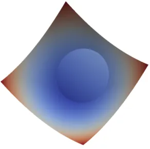
Figure 3: Sloshing of a drop on a parabolic support – State obtained after one revolution (very close to the initial state).
6.1. Rotation in a paraboloid
This first test case consists in calculating the uniform rotation of a circular drop on a support of parabolic shape (see Figure 3). The computational domain is (0, L)×(0, L) and the elevation of the support is:
z = −h01 − (x − L2)2− (y −L2)2,
with L = 4 and h0=0.1. The fluid height is given by
h = h0 max0, (x −L2) cos(ωt) + (y −L2) sin(ωt) − z − 0.5,
and the velocity is
u = 12ω − sin(ωt) cos(ωt) .
It is then easy to check that the mass and momentum balance equations are verified provided that ω2 = 2 g h0. The solution is thus regular, and this test features a regular topography
and dry zones (i.e. zones where h = 0). We compare the numerical and theoretical height obtained after one rotation (i.e. ωt = 2π), for different uniform grids and with a time step δt = δx/8. (the maximal speed of sound and the maximal velocity are both close to 1); results are gathered in the following table:
grid error (discrete L1norm)
100 × 100 3.02 10−3
200 × 200 1.54 10−3
400 × 400 0.896 10−3
800 × 800 0.511 10−3
We observe an order of convergence between 0.8 and 1, which is consistent with a first-order approximation of the fluxes and the time derivative.
6.2. A dam-break problem
In this test, the computational domain is:Ω =(0, 200) × (0, 200) \ Ωwwith Ωw=(95, 105) × (0, 95) ∪ (95, 170) × (0, 200).
The fluid is supposed to be initially at rest, and the initial height is h = 10 for x1≤ 100 and h =
5 for x1>100. A zero normal velocity is prescribed at all the boundaries of the computational
domain. The computation is performed with a mesh obtained from a 1000×1000 regular grid, by removing the cells included in Ωw. The time step is δt = δx/25 (the maximal speed of
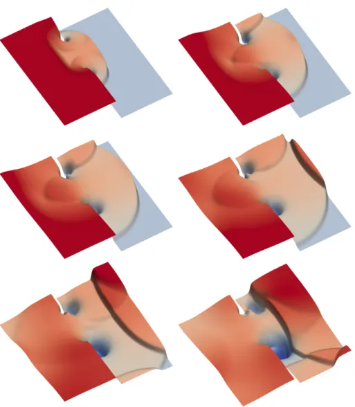
sound and the maximal velocity are both close to 10). The obtained fluid height is shown at different times on Figure 4; they confirm the efficiency of the scheme, and its capability to deal with reflexion phenomena very simply (i.e. just by setting the normal velocity at the boundary to zero, by contrast with schemes based on Riemann solvers which need to implement fictitious cells techniques).
Acknowledgements
The authors would like to thank Robert Eymard and Thierry Gallouët for several interesting discussions.
References
[1] Arakawa, A., and Lamb, V. A potential enstrophy and energy conserving scheme for the shallow water equations. Monthly Weather Review 109 (1981), 18–36.
[2] Bonaventura, L., and Ringler, T. Analysis of discrete shallow-water models on geodesic delaunay grids with c-type staggering. Monthly Weather Review 133, 8 (2005), 2351–2373.
[3] Bouchut, F. Nonlinear Stability of finite volume methods for hyperbolic conservation laws. Birkhauser, 2004.
[4] CALIF3S. A software components library for the computation of fluid flows.
https://gforge.irsn.fr/gf/project/califs.
[5] Doyen, D., and Gunawan, H. An explicit staggered finite volume scheme for the shallow water equations. In Finite volumes for complex applications. VII. Methods and theoret-ical aspects, vol. 77 of Springer Proc. Math. Stat. Springer, Cham, 2014, pp. 227–235.
Figure 4: Partial dam break – Height obtained at t = 4, t = 8, t = 10, t = 12, t = 16 and t = 20 with a mesh obtained (by supression of the zones associated to the obstacles) from a 1000 × 1000 regular grid. In the last Figure (t = 20), the obtained minimal and maximal heights are h = 2.149 and h = 9.306 respectively.
[6] Gallou¨et, T., Herbin, R., and Latch´e. On the weak consistency of finite volumes schemes for conservation laws on general meshes. under revision (2019). Available from: https://hal.archives-ouvertes.fr/hal-02055794.
[7] Gallou¨et, T., Herbin, R., Latch´e, J.-C., and Mallem, K. Convergence of the marker-and-cell scheme for the incompressible Navier-Stokes equations on non-uniform grids. Foundations of Computational Mathematics 18 (2018), 249–289.
[8] Gunawan, H. Numerical simulation of shallow water equations and related models. PhD thesis, Université Paris-Est and Institut Teknologi Bandung, 2015.
[9] Herbin, R., Kheriji, W., and Latch´e, J.-C. On some implicit and semi-implicit staggered schemes for the shallow water and Euler equations. ESAIM: Mathematical Modelling and Numerical Analysis 48 (2014), 1807–1857.
[10] Herbin, R., Latch´e, J.-C., and Nguyen, T. Explicit staggered schemes for the compress-ible Euler equations. ESAIM: Proceedings 40 (2013), 83–102.
[11] Herbin, R., Latch´e, J.-C., and Nguyen, T. Consistent segregated staggered schemes with explicit steps for the isentropic and full Euler equations. ESAIM: Mathematical Modelling and Numerical Analysis 52 (2018), 893–944.
[12] Stelling, G., and Duinmeijer, S. A staggered conservative scheme for every Froude number in rapidly varied shallow water flows. International Journal for Numerical Methods in Fluids 43 (2003), 1329–1354.
R. Herbin and Y. Nasseri
Aix-Marseille Université, Institut de Mathématiques de Marseille, 39 rue Joliot Curie
13453 Marseille
[email protected] [email protected]
J.-C. Latché
Institut de Radioprotection et Sûreté Nucléaire, 13115, Saint-Paul-lez-Durance [email protected] N. Therme CEA/CESTA 33116, Le Barp, France [email protected]