Coupling the Soil-Vegetation-Atmosphere-Transfer Scheme ORCHIDEE to the agronomy model STICS to study the influence of croplands on the European carbon and water budgets

HAL Id: hal-00886031

https://hal.archives-ouvertes.fr/hal-00886031

Submitted on 1 Jan 2004

HAL is a multi-disciplinary open access

archive for the deposit and dissemination of

sci-entific research documents, whether they are

pub-lished or not. The documents may come from

teaching and research institutions in France or

abroad, or from public or private research centers.

L’archive ouverte pluridisciplinaire HAL, est

destinée au dépôt et à la diffusion de documents

scientifiques de niveau recherche, publiés ou non,

émanant des établissements d’enseignement et de

recherche français ou étrangers, des laboratoires

publics ou privés.

Scheme ORCHIDEE to the agronomy model STICS to

study the influence of croplands on the European carbon

and water budgets

Nathalie de Noblet-Ducoudré, Sébastien Gervois, Philippe Ciais, Nicolas

Viovy, Nadine Brisson, Bernard Seguin, Alain Perrier

To cite this version:

Nathalie de Noblet-Ducoudré, Sébastien Gervois, Philippe Ciais, Nicolas Viovy, Nadine Brisson, et

al.. Coupling the Soil-Vegetation-Atmosphere-Transfer Scheme ORCHIDEE to the agronomy model

STICS to study the influence of croplands on the European carbon and water budgets. Agronomie,

EDP Sciences, 2004, 24 (6-7), pp.397-407. �10.1051/agro:2004038�. �hal-00886031�

DOI: 10.1051/agro:2004038

Original article

Coupling the Soil-Vegetation-Atmosphere-Transfer Scheme

ORCHIDEE to the agronomy model STICS to study the influence

of croplands on the European carbon and water budgets

Nathalie de N

-D

_{*, Sébastien G}

_{, Philippe C}

_{, Nicolas V}

_{, Nadine B}

_,

Bernard S

, Alain P

a _{Laboratoire des Sciences du Climat et de l’Environnement (LSCE), Bât. 701, Orme des Merisiers, 91191 Gif-sur-Yvette Cedex, France}

b _{Institut National de Recherche Agronomique (INRA), Unité Climat, Sol et Environnement, Domaine St Paul, Site Agroparc, 84914 Avignon Cedex 9, France} c _{INAPG, Chaire de Bioclimatologie, Département AGER, 16 rue Claude Bernard, 75231 Paris Cedex 05, France}

(Received 16 June 2003; accepted 14 May 2004)

Abstract – Agriculture is still accounted for in a very simplistic way in the land-surface models which are coupled to climate models, while the area it occupies will significantly increase in the next century according to future scenarios. In order to improve the representation of croplands in a Dynamic Global Vegetation Model named ORCHIDEE (which can be coupled to the IPSL1 climate model), we have (1) developed a procedure which assimilates some of the variables simulated by a detailed crop model, STICS, and (2) modified some parameterisations to avoid inconsistencies between assimilated and computed variables in ORCHIDEE. Site simulations show that the seasonality of the cropland-atmosphere fluxes of water, energy and CO₂ is strongly modified when more realistic crop parameterisations are introduced in ORCHIDEE. A more realistic representation of wheat and corn croplands over Western Europe leads to a drying out of the atmosphere at the end of summer and during autumn, while the soils remain wetter, specially at the time when winter crops are sowed. The seasonality of net CO₂ uptake fluxes is also enhanced and shortened.

global biosphere modelling / heat and water fluxes / water balance / carbon balance / phenology

1. INTRODUCTION

Terrestrial vegetation affects atmospheric composition, sur-face energy budgets and hence climate through exchanges of water, energy, momentum, CO2, CH4, N2O and chemically active species (NH₃, NO_x), and aerosols. Changes in the veg-etation composition and in land cover alter those fluxes and therefore have the potential to feed back on the atmospheric cir-culation and composition.

Many authors have outlined the importance of vegetation in influencing past climates at the regional level. In North Africa, for example, greater summer insolation received 6 000 years ago induced a deepening of the thermal trough over the Sahara, which increased the summer monsoon flow and rainfall, thereby allowing for the growth of grass (e.g. [23]). The latter in turn amplified the process initiated by the change in summer insolation (e.g. [7, 9, 25, 35]).

Another example is the transition between boreal forest and tundra at high northern latitudes which was located at a more southerly position (than today) during the last glacial inception (e.g. 115 000 years ago) and further north during the

mid-Holocene warm period. The last glaciation would not have started without the southward migration of grasses and shrubs, at the expense of forests, inducing a positive feedback via snow-covered vegetation on the insolation-induced cooling (e.g. [10, 16]).

For a long time mankind has modified the landscape [37], clearing forests to grow crops and pastures, and build houses and cities. Numerical simulations of the impact of tropical deforestation in South America have found decreased eva-potranspiration rates, increased surface temperatures, and sig-nificant changes in water vapour advection from the Atlantic, resulting in changes in the distribution of rainfall over northern South America (e.g. [17, 31, 32, 39]). Tropical land-use changes have been shown to impact on the climate in a similar mode to during an El Niño event [30].

Deforestation also results in large emissions of CO2 into the atmosphere, thereby enhancing the greenhouse warming effect [21].

Other studies have examined the effects of changes in extra-tropical land cover on regional climates. Eastman et al. [13], for example, simulated the effect of grazing suppression in the

* Corresponding author: noblet@lsce.saclay.cea.fr

Great Plains of the United States after European settlement and found a cooling response in daily maximum temperature asso-ciated with reduced precipitation. Heck et al. [20] showed that the suppression of European forests that took place during the past 2 000 years probably led to a moister and cooler spring fol-lowed by a drier and warmer summer in the Mediterranean region. Copeland et al. [8] have examined the effect of cropping in the United States and found that current land use was causing the summertime surface conditions to be warmer and wetter than under natural land cover.

Global-scale simulations have also been carried out using simplified climate models (e.g. [5, 26]) or more complex ones (e.g. [1, 6, 19]) and all agreed on the role of land-cover changes (induced by land use) in cooling the Earth's surface when for-ests are converted to grasslands, thereby opposing the green-house warming effect. Figure 1 illustrates the potential impact that cultivated areas may have on the climate of Europe. The simulation, which was carried out using version 5.3 of the IPSL model (http://www.ipsl.jussieu.fr/~omamce/IPSLCM4), com-pares the climate with present-day land cover with climate in a scenario where natural vegetation is potential in all places (i.e. before the extensive European deforestation of the Middle Ages). We simulate milder winters when crops are present, with wetter conditions in northern Europe and drier conditions in the Mediterranean, resulting from an increased advection of heat and moisture from the tropical Atlantic. Summers, on the other hand, are cooler due to increased latent heat flux. Euro-pean crops do indeed transpire more than a natural forest due to their enhanced photosynthetic capacity that induces a larger canopy conductance. But this numerical experiment, like all the others reported earlier, assumed crops to have the same sea-sonality as a natural grass (see Sect. 2).

Moreover, future scenarios of changes in vegetation distri-bution from the IMAGE project [36], resulting from an inte-grated assessment approach, outline the almost total disappear-ance of forests in equatorial and tropical Africa in about 40 to 100 years from now, while part of the temperate crops and pas-tures will be re-forested. The climate impacts of such projected land-cover changes are largely unknown.

Replacing forests with crops also has an indirect effect via changes in the atmospheric greenhouse gas concentrations. Cutting forests to establish arable lands and plowing natural grasslands result in a disturbance of carbon stocks, augmenting erosion and causing net release of CO₂ to the atmosphere. This loss can be slowed down and even offset by several carbon sequestering practices (e.g. reduced or no tillage, manure appli-cation and fallow).

The role of croplands in adding carbon to or removing it from the atmosphere is still highly uncertain, and depends on practice [34], and past land-use history. In the case of European crop-lands, Vleeshouwers et al. [38], using the CESAR model forced with statistical data and empirical processes, concluded a car-bon source of 400 TgC y–1, that is, ~40% of fossil fuel emis-sions. The uncertainty on this number, however, is very large (on the order of the mean) as discussed in Janssens et al. [22]. The poor representation of crops and pastures in biogeo-chemical and soil-vegetation-atmosphere transfer global mod-els justifies the improvement of the description of those eco-systems. In a former paper [18] we presented the specific changes we made to our original model (ORCHIDEE) to parameterise crops better. The approach is briefly recalled in Section 2, with a quick presentation of the models. Section 3 shows the performances of the updated model at some selected sites. Section 4 discusses the influence of croplands on the European carbon and water budget.

Figure 1. Differences in simulated surface air temperature (°C) in (a) winter (December-January-February) and (b) summer (June-July-August), and (c) in simulated winter precipitation (mm/day) between a simulation of the present-day climate (using version 5.3 of the LMD atmospheric general circulation model) with actual vegetation and a simulation of the present-day climate where agricultural land has been replaced by potential vegetation (mainly forests).

2. MODELS AND COUPLING STRATEGY

The objective is to improve the generic, spatially explicit, carbon-water-energy model ORCHIDEE [24] for use in studies estimating the changes in global carbon sources/sinks and cli-mate, due to human-induced changes in land cover. Instead of introducing specific parameterisations for crops in ORCHIDEE, we rather decided to make use of an existing crop model, STICS [3, 4], specifically designed to represent as accurately as pos-sible the yield and phenology of crops. Only wheat and corn, two dominant crop species grown in Europe, are considered in this preliminary work.

In the “coupled” approach, some variables initially simu-lated by ORCHIDEE are replaced with the ones computed by STICS. This allows us to use all future improvements that will be made in STICS, with minimum further adjustments of ORCHIDEE. Using STICS in place of ORCHIDEE to force the atmosphere was not possible since the STICS daily time-step lacks adequate description of diurnal fluxes as required by cli-mate models (e.g. water, heat, momentum and CO₂).

2.1. ORCHIDEE (“Organising Carbon and Hydrology In Dynamic EcosystEms”)

ORCHIDEE [24] is built on the Soil-Vegetation-Atmos-phere Transfer Scheme SECHIBA [11, 12], which was designed to be coupled to atmospheric general circulation mod-els. It computes the “instantaneous” fluxes of momentum, heat, water, the soil water budget and the surface energy budget. Its time-step is half an hour, to ensure numerical stability and to adequately represent the diurnal cycle. The carbon cycle has been added to SECHIBA based on a number of previously pub-lished works (e.g. Botta et al. [2] for the phenology; Friedling-stein et al. [15] for allocation processes). Photosynthesis and respiration have been included in SECHIBA since these proc-esses have to be computed at the shortest time-step, while leaf shooting, allocation, litter production, decomposition and the fire index are simulated using a daily time-step. A third module (with a time-step of one year) was taken from the LPJ model [33] to compute the vegetation dynamics (evolution from one vegetation type to another one). In this study, this module was turned off since the distribution of vegetation was always pre-scribed.

Vegetation types are grouped into ten natural plant func-tional types (PFTs) (evergreen and deciduous trees and C₄ and C₃ grasses), bare soil, and two “super-grasslands”, C3 and C4, which we name crops but which only differ from natural grass in their prescribed higher rates of carboxylation and Rubisco regeneration. Several PFTs can coexist within the same grid box (also referred to as a mosaic vegetation). They all share the same climate forcing but compute fluxes depending on their own properties. The fluxes are thereafter averaged before enter-ing the first atmospheric level.

2.2. STICS (“Simulateur mulTIdisciplinaire pour les Cultures Standard”)

STICS2 [3, 4] is a modular crop model developed by INRA (France) as a tool for computing crop yield (amount and qual-ity) and environmental variables (water and nitrogen losses).

It relies on empirically characterised processes and simulates, daily, the behaviour of crops in the soil-plant-atmosphere con-tinuum (above-ground biomass and its nitrogen content, leaf area index, number of harvested grains and their biomass, soil water and nitrogen budgets, root profile and density, etc.). STICS has been validated and applied to a variety of crops (wheat, corn, tomato, banana, soybean, grassland, vineyards etc.) without any structural changes. Only some parameters and the technical agenda (sowing date, amount of fertilisers, amount of irrigation, etc.) need to be updated depending on the chosen crop type.

STICS is divided into seven modules. The first three calcu-late the above-ground state of crops (leaf area index and bio-mass, and allocation to grains), the last four the soil water and nitrogen budgets (there is no explicit soil carbon budget), the root growth and the transfers of water and nutrients between the soil and the above-ground biomass through the roots

2.3. Coupling strategy

At two sites (wheat and corn in France) we compared the above-ground biomass (hereafter AGB) simulated by ORCHIDEE in its standard version and by STICS (Fig. 2), as well as the observed AGB. This variable is directly related to foliage den-sity (or leaf area index) which is of particular importance since

2 _{In this study, we have used version 4.0 of STICS.}

Figure 2. Time evolution of observed (triangles) and simulated above-ground biomass (gC/m2). Simulated values from STICS are plotted using the thick black line, while results from ORCHIDEE are plotted using the dark grey line (ORCHIDEE-STICS) and the dotted grey line (ORCHIDEE). Results are shown for (a) winter wheat at Grignon in 1995, and (b) corn in Poitou-Charentes in 1996.

it feeds back on albedo, roughness length and canopy conduct-ances and thereby on turbulent fluxes of latent and sensible heat, and on canopy photosynthesis. ORCHIDEE represents wheat as a natural C3 grass but with enhanced photosynthesis (Fig. 2a) and the pertaining AGB thus closely follows the cli-matic conditions: a germination in spring and a maximum in late summer. In the real world, wheat is sown in October-November, starts to germinate before winter and reaches max-imum AGB in spring before being harvested in early summer. For corn, even if the AGB timing is not as crucial (Fig. 2b) since this cereal is only sown in spring and therefore germinates at the same time as a natural grass, the amplitude of the simu-lated AGB is underestimated by ORCHIDEE, despite the pre-scribed increased photosynthetic capacity which allows more productivity than in a natural grassland. Moreover, the simu-lated growing season is too long in our model.

The reasons for all these shortcomings of ORCHIDEE relate to crop-specific processes present in STICS (implicitly or explicitly) and absent from ORCHIDEE such as selection of crop species, use of fertilisers to maximise grain yield over short growing cycles, agricultural practices (e.g. ploughing, sowing date, irrigation, harvest date and tillage).

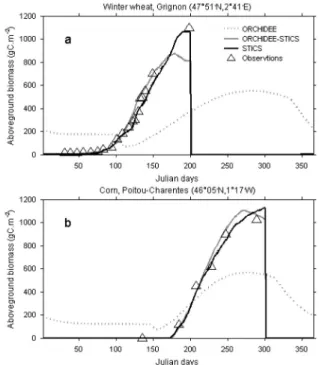
The strategy we adopted to improve ORCHIDEE is to use some of STICS’ outputs in place of the ones that are either badly simulated (e.g. leaf area index; hereafter LAI) or missing (e.g. nitrogen stress). Each model is run simultaneously and forced with the same atmospheric forcing and surface characteristics (see Fig. 3 for schematic diagram). Each day STICS provides ORCHIDEE with values of leaf area index, root profile, nitro-gen stress and vegetation height. The parameterisations that had to be updated in ORCHIDEE to maintain a basic consist-ency with input variables from STICS are (1) the allocation pro-cedure and leaf senescence, to ensure consistency between LAI (resp. root profile) and leaf biomass (resp. root biomass), and (2) the soil moisture stress to ensure consistency with the root profile from STICS. Detailed descriptions of these changes and of their impact on the simulated fluxes and biomass can be found in Gervois et al. [18].

We will hereafter refer to our modified version of ORCHIDEE as ORCHIDEE-STICS.

3. EVALUATION AT SPECIFIC SITES

3.1. Simulated above-ground biomass at two sites in France

The simulated above-ground biomass using ORCHIDEE-STICS is shown in Figure 2, where a significant improvement can be seen. The biomass increases up to day 160 for winter wheat and day 265 for corn, then decreases following the decrease in leaf area index and the removal of senescent leaves by litterfall. In STICS (and in reality), on the other hand, the decrease in above-ground biomass does not start until harvest. Moreover, the above-ground biomass continues to increase because the filling of grains starts once the LAI has reached its climax. In ORCHIDEE-STICS the allocation of assimilates to grains takes place as soon as net primary production is positive (i.e. since leaf shooting). This is why there is a slight

overesti-mation of biomass during the growing season in ORCHIDEE at both sites. The simulated grain biomass at harvest is, how-ever, similar in both models (~380 gC/m2 for winter wheat and ~550 gC/m2 for corn) and matches the observed values well. Outside the growing season, ORCHIDEE predicts constant above-ground biomass for corn, while there is no biomass in both STICS and the data. This “residual” biomass is an inert reserve put aside in ORCHIDEE, from the harvested grains, to start the next season’s growth of leaves. This reservoir therefore mimics the amount of seeds spilled on the ground by the farmer. It is almost null for wheat since emergence occurs in winter, and despite the very small amount of leaves some primary pro-ductivity is simulated and allocated to the growth of leaves (reserves are therefore not really necessary in that case).

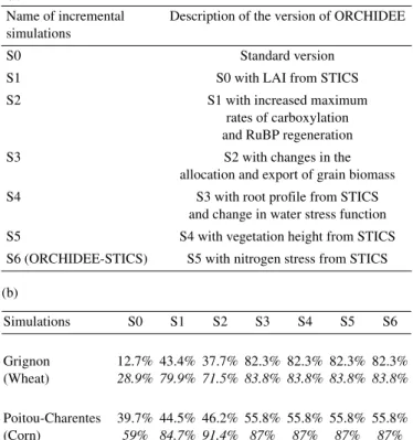
Table Ia summarises the incremental changes that we made to ORCHIDEE. The two modifications that led to the major changes in total aerial biomass for the wheat and corn sites (Tab. Ib) are the LAI values taken from STICS (from simula-tion S0 to S1), and the change in allocasimula-tion (from S2 to S3). After the change in allocation was made, there was no subse-quent alteration of the simulated aerial biomass. The changes from S0 to S1 are the most significant improvements in ORCHIDEE if one focuses on the growing season only (num-bers in italic in Tab. Ib). Very great changes from S5 to S6 were obtained at a site where a strong nitrogen stress was felt. This result is not presented here but discussed in Gervois et al. [18].

3.2. Simulated water and net CO₂ fluxes at two sites in North America

With ORCHIDEE-STICS being able to realistically simu-late the biomass growth, we then checked the model against in situ continuous flux measurements by the eddy covariance tech-nique. Two sites of the Ameriflux network [14] were chosen (Fig. 4): a winter wheat field in Ponca (Oklahoma, 97°08’W / 36°46’N), and a corn field in Bondville (Illinois, 88°17’W / 40°00’N). The meteorological data used as input were those measured at a half-hourly time-step in 1997. Sowing occurred on October 14th 1996 in Ponca (George, pers. comm.), and the 1st of May 1997 in Bondville (Meyers, pers. comm.). All other data on agricultural practices such as the timing and amount of irrigation or fertilisers (if any) were not available and we let STICS compute its own needs depending on its simulated water and nitrogen stress.

In Bondville (corn) the simulated LAI is in very good agree-ment with the observations (Fig. 4f) and controls the net eco-system exchange of CO₂ (NEE) from source to sink (and vice versa, Fig. 4d). Soon after the LAI has reached its maximum value (~day 180), the simulated carbon uptake is not as high as observed, probably reflecting an overestimated water stress (though not sufficient enough for STICS to initiate irrigation) in our simulation. Evapotranspiration (ETR) at peak LAI in ORCHIDEE-STICS (Fig. 4e) is much higher than observed, reducing strongly, and rapidly, the available soil water. Soon after that episode, the simulated ETR decreases together with the CO₂ sink, due to a strong decrease in gross photosynthesis (going from 19.1 to 15.9 gC/m2/day, while autotrophic respi-ration goes from 7.1 to 6.2 gC/m2/day, and heterotrophic res-piration from 2.1 to 2.2 gC/m2/day). At peak LAI, though, the simulated NEE was remarkably similar to that observed. The

large difference in ETR between the model and observations may result from the selected crop type. We did indeed choose the same characteristics for this American corn type as for the French site in Poitou-Charentes (Sect. 3.1). American corn may be more resistant to rainfall deficit and have a greater water-use efficiency, thereby preventing water loss while preserving large rates of photosynthesis. The strongest rainfall deficit, between days 220 and 230, causes a realistic model response (decrease in ETR and reduced NEE), although about 10 days earlier than observed. Here again, the water stress (even if small) experienced by our model prior to this event is respon-sible for this rapid response to rainfall, while in reality the stress

was probably felt only after ETR had extracted enough water from the soil.

In Ponca the winter wheat field acts as a net sink of atmos-pheric CO₂ between day 40 and day 140, and as a net source the rest of the year (Fig. 4a). This change in behaviour (with respect to CO₂) occurs shortly before harvest (Fig. 4c), at a time when most leaves are senescent and photosynthesis cannot compensate for respiration. ORCHIDEE-STICS reproduces very well the timing from sink to source but with a delay of about 6 days, which we assume is due to a similar delay in the onset of leaves, as suggested by both the too smooth an increase in CO₂ uptake and the too slow an increase in ETR (Fig. 4b).

Figure 3. Schematic of ORCHIDEE-STICS, an altered version of ORCHIDEE [24]. ORCHIDEE-STICS incorporates agro-ecosystems using crop phenology, crop management (e.g. fertiliser application, irrigation) and nitrogen cycling. Dotted arrows and bold text in dotted boxes indicate the variables that are simulated by STICS and assimilated in ORCHIDEE. Text in italic and underlined indicates parameterisations of ORCHIDEE that have been updated. Lightly dashed boxes refer to fast processes (time-step smaller than 1 hour), while grey boxes refer to processes/variables computed daily. White boxes show prescribed variables.

The amplitude of both quantities, though, as well as the length of the crop season, is well reproduced by ORCHIDEE-STICS. The rainfall deficit experienced by day 90 results in a sharp decrease in ETR and sharp decrease in NEE in the model, in good agreement with the observations. The magnitude of this stress event is smaller, though, in ORCHIDEE-STICS since the simulated area of standing leaves is still quite low (if our hypothesised delay is correct, the real-world LAI should be somewhat larger).

4. INFLUENCE OF CROPLANDS

ON THE CONTINENTAL SCALE EUROPEAN WATER AND CARBON BUDGETS

4.1. Designing a set of simplified simulations

We applied ORCHIDEE-STICS to Western Europe (36°N– 55°N; 10°W–19°E) where arable land amounts to a large frac-tion of the total land cover (~37.5% of Europe; [27]) and is

therefore expected to have a significant impact on regional cli-mates and on the CO2 fluxes.

Our purpose in this paper is to understand how a better rep-resentation of cropland will affect the estimated carbon and sur-face energy budgets.

We used as input the gridded present-day climate data derived from the ATEAM European-funded project (EVK2-2000-00075; http://www.pik-potsdam.de/ateam/). The vegeta-tion map is based on CORINE land cover (1995; http:// reports.eea.eu.int) for the distribution of natural vegetation and the area occupied by crops, combined with information from the FAO regarding the partitioning between C3 and C4 crops in each country (http://www.fao.org).

Two simulations were carried out, at 1° by 1° horizontal res-olution:

♦ NOCROP using the standard version of ORCHIDEE (where crops behave more like a natural grass),

♦ CROP using ORCHIDEE-STICS.

In upscaling to the continent, we had to make some arbitrary simplifications regarding the technical agenda which was not available on this scale (or at least not easily available). We chose, in this very first attempt, to describe all C3 crops as win-ter wheat, and all C4 ones as corn. The sowing date was fixed to October 1st for wheat, and once weekly mean temperature goes above 10 °C for corn. We let fertilisation and irrigation be computed by STICS once the nitrogen and water availability went below a certain threshold. The harvest date is computed using the growing-degree day concept. For all characteristics describing the specificities of each crop (e.g. GPP thresholds and conversion efficiency), we used the same ones as for the French sites described in Section 3. Remark also that the carbon simulations are done under equilibrium conditions, i.e. the annual carbon balance of the crop systems is zero, thus ignoring the effects of the historical climate, CO₂ and management changes on the carbon cycling. Thus the only predictive quan-tity is the simulated seasonality of NEE.

We are aware that these simplifications are very crude, but we believe that, given the enormous change in seasonality obtained when comparing both versions of ORCHIDEE (see Sects. 2 and 3), the arbitrary choices we have made may only have second-order effects. Moreover, it seems obvious from Table I that the biggest improvement that can be made to a glo-bal model concerns LAI seasonality and appropriate redistri-bution of photosynthate products.

4.2. Seasonal evolution of leaf area index

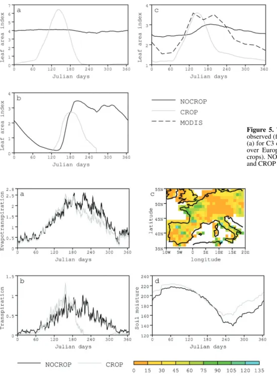
Leaf area index (LAI) is of primary importance since many other variables depend upon its value. The time evolution of LAI, averaged over the model domain, is plotted in Figure 5 for both versions of ORCHIDEE, and compared with satellite data (Fig. 5c). There is almost no seasonal cycle for wheat (Fig. 5a) in the standard simulation (NOCROP), and the grow-ing season is too long for corn (Fig. 5b) in the absence of har-vest. Because the area covered by C3 crops is quite large over Europe (~35% compared with ~2.5% for C4 crops), the mean LAI computed considering all other PFTs (natural vegetation) is strongly influenced by winter wheat (Fig. 5c).

Table I. Summary of the degree of agreement (expressed in %) between the above-ground biomass simulated by STICS (almost equal to observations) and the one simulated by different versions of ORCHIDEE. (a) Summary of the incremental (step-by-step improve-ment) versions of ORCHIDEE which are fully described in [18]. (b) The degree of agreement is computed as the integral of the common space covered by the above-ground biomass divided by the integral of the total space covered (including both STICS and ORCHIDEE). In plain text calculations were made throughout the year, while in italic calculations were made for the crop season (from actual emergence to harvest) only.

(a)

Name of incremental simulations

Description of the version of ORCHIDEE

S0 Standard version

S1 S0 with LAI from STICS

S2 S1 with increased maximum

rates of carboxylation and RuBP regeneration

S3 S2 with changes in the

allocation and export of grain biomass S4 S3 with root profile from STICS

and change in water stress function S5 S4 with vegetation height from STICS S6 (ORCHIDEE-STICS) S5 with nitrogen stress from STICS (b) Simulations S0 S1 S2 S3 S4 S5 S6 Grignon (Wheat) 12.7% 28.9% 43.4% 79.9% 37.7% 71.5% 82.3% 83.8% 82.3% 83.8% 82.3% 83.8% 82.3% 83.8% Poitou-Charentes (Corn) 39.7% 59% 44.5% 84.7% 46.2% 91.4% 55.8% 87% 55.8% 87% 55.8% 87% 55.8% 87%

When compared with the LAI derived from the MODIS sat-ellite observations [28], it is obvious that using ORCHIDEE-STICS (CROP) results in a significant improvement. The monthly LAI, though, seems to be underestimated in winter and the growing season seems too short (by about 60 days). During wintertime, this discrepancy could result from the regrowth of grass on cultivated lands, which is not accounted for in our model. The shorter growing season simulated could result from the choice we made to grow only winter wheat, instead of hav-ing part of the C3 crops behav-ing sprhav-ing fields. The first peak in satellite observations (~day 120) is indeed indicative of the maximum growth of winter crops, while the second one (~day 210) may be related to spring crops, prairies and decid-uous trees. It is obvious from these results that we need to include more than just winter crops in CROP in the future improvement of our code.

4.3. Energy and water balance

The seasonal evolution of evapotranspiration (ETR), as dis-played in Figure 6a for both CROP and NOCROP simulations,

does not parallel the behaviour of leaf area index (Fig. 5c). ETR values are indeed quite similar in both versions from November to June. The soil is not depleted in moisture during that period since it has replenished during winter and the water demand is not very great in spring. The ETR is therefore quite close to the potential rate. Moreover, the change in canopy resistance with increased LAI, when comparing both model versions, is small and results in a slight increase in ETR in CROP.

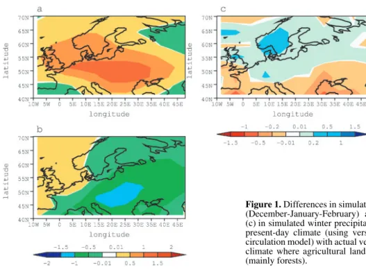
However, from early July until the end of October, the ETR rates simulated in NOCROP are larger than those simulated in CROP, reflecting the presence of leaves in NOCROP, in areas covered with winter wheat, while bare soil is the only potential source of evaporation in CROP (Fig. 6b). The annually cumu-lated difference of ETR between the standard and the improved version of our code (still averaged over Europe) amounts to 42 kg of water per m2 of soil, of which 41 kg/m2 arise from the four months of obvious discrepancy (July to October). Inte-grated over our European domain, 1.64 × 1011 m3 of water are lost in one year for the atmosphere, i.e. about 1% of its maxi-mum storage value (which is 13 × 1012 m3/year according to estimates from Perrier et al. [29]) .

Figure 4. Time evolution of a number of observed (thick black line) and simulated (thin dark grey line for ORCHIDEE-STICS and dotted grey line for ORCHIDEE) variables at the two American sites: winter wheat in Ponca on the left side and corn in Bondville on the right side. (a) and (d) Net ecosystem exchange (gC/m2/day). Negative values represent a sink of CO₂ with respect to the atmosphere, while positive values represent a source. (b) and (e) Total evapotranspiration (mm/day); (c) and (f) leaf area index. All values are presented as 5-day running means to smooth out very high frequencies.

These results imply that more accurate representation of crop phenology leads to a smaller loss of water to the atmos-phere, which therefore should dry out in the absence of feed-backs. The soil, on the other hand, remains wetter when crops are more realistically simulated. Differences are largest at the end of September (Fig. 6c-d) once the cropping season has stopped and right before the start of the next season. The areas where storage of water is the largest in CROP are those where the proportion of C3 cover is also the largest (not shown). At the end of May, on the other hand, although winter wheat has already been quite productive in CROP, the soil remains quite (and similarly) wet in both versions (Fig. 6d).

The large seasonal and annual changes in ETR that are described above are partly compensated by changes in sensible heat which slightly increases from July until October in CROP (Fig. 7a) and by the warming of the land surface (Fig. 7b), resulting in more thermal loss.

4.4. Carbon budget

Both CROP and NOCROP simulations assume equilibrium of all carbon reservoirs, and therefore the net annual NEE is zero. Nevertheless, we observe in Figures 8a–c that when crops are included in the model, the seasonality of photosynthesis

Figure 5. Time evolution of the simulated and observed (from MODIS satellite) leaf area index. (a) for C3 crops; (b) for C4 crops; (c) mean LAI over Europe, combining all PFTs (natural and crops). NOCROP is plotted using the black line, and CROP using the grey line.

Figure 6. Simulated water budget over Europe. (a) simulated time evo-lution of mean evapotranspiration (mm/day). (b) simulated time evo-lution of mean transpiration of C3 crops (mm/day). (c) Mean differ-ence (CROP – NOCROP) in total soil moisture (mm) at the end of the growing time (averaged between mid-September and mid-October). (d) simulated time evolution of mean total soil moisture over Europe (mm). For time evolutions, NOCROP is plotted using the black line, and CROP using the grey line.

(GPP) is enhanced, resulting in an increase in the seasonal peak-to-peak amplitude of GPP by ~60% compared with NOCROP (respective maximum GPP values are 11 gC/m2/yearin CROP and 7.9 gC/m2/year in NOCROP). Parallel to the simulated LAI seasonality, GPP remains close to zero prior to the start of plant growth (day 60) and after harvest (day 200), unlike in NOCROP where crops behave like grasslands, growing all year round.

The seasonal cycle of NEE is also enhanced (Fig. 10d), and primarily reflects the GPP increase in Figure 10c. The NEE enhancement quantified by the difference between CROP and NOCROP cumulated between day 60 and day 190 amounts to 171 gC/m2 (NEE in CROP is ~5.5 times higher than in NOCROP), compared with 175 gC/m2 (~25% of the NOCROP value) for the GPP enhancement. This shows that GPP, rather than respiration, controls NEE during the crop-growing season. This corroborates the results obtained at the North American flux sites. Note that global inversion studies using atmospheric CO2 concentration measurements to infer the large-scale dis-tribution of sources and sinks of CO₂ all calculate an increased seasonality of NEE in Europe when compared with the first guess fluxes where crops are not accounted (Rivier pers. comm.). This indirectly corroborates the increased seasonality of NEE over Europe found in the CROP run, although inver-sions remain too coarse to separate crops and forests within Europe.

Interestingly, in the two months following the harvest of the C3 crops (day 190-day 310), NEE in the CROP run is a larger source to the atmosphere compared with the NOCROP run. This is because larger amounts of assimilates formed during the growing season are laid off to the ground where they decom-pose rapidly.

Figure 8. Time evolution of simulated components of the carbon cycle, expressed in gC/m2 and averaged over Europe. (a) Mean gross primary production (GPP) of C3 crops. (b) Mean GPP of C4 crops. (c) European GPP (cumulated over all PFTs). (d) European net ecosystem productivity (cumulated over all PFTs). NOCROP is plotted using the dark line, and CROP using the grey line.

Figure 7. Time evolution of the simulated (a) sensible heat flux (W/ m2), averaged over Europe. NOCROP is plotted using the dark line, and CROP using the grey line. (b) difference in surface soil temperature between CROP and NOCROP, averaged over Europe. Negative values indicate colder temperature when crops are more adequately simulated.

The equilibrium soil carbon stocks are smaller in CROP (108 t/ha) than in NOCROP (152 t/ha) due to the export of har-vested biomass in ORCHIDEE-STICS (see simulation S3 in Tab. Ia). To study the behaviour of croplands as carbon net annual sinks or sources, we would need to run longer simula-tions with changing management, CO₂ and climate. The only comment we can make here is that carbon uptake by croplands occurs during a shorter time period and is more efficient in the CROP run.

5. CONCLUSION

We modified a global and dynamic vegetation model named ORCHIDEE to account for croplands better, using knowledge from the STICS crop model. Specific outputs from STICS describing the phenological state of agro-ecosystems are pre-scribed in ORCHIDEE which then recomputes the carbon, water and energy fluxes.

Application of ORCHIDEE-STICS over Western Europe shows that accounting for crops in that manner results in a much shorter growing season, leading to a drier atmosphere, wetter soils, and warmer soil temperatures in autumn with more sen-sible heat emitted to the atmosphere. The seasonal cycle of NEE is increased as reflecting enhanced photosynthesis during the crop-growing season, and results altogether in a shorter but more efficient period for carbon uptake.

Implications of theses changes on the European climate and on atmospheric CO₂ composition needs to be (and will be) stud-ied using a general circulation model of the atmosphere coupled to a land-surface scheme. ORCHIDEE is already coupled to the LMDz atmospheric model developed at IPSL and is therefore an adequate candidate for further testing.

Acknowledgements: This work was carried out at the Laboratoire des

Sciences du Climat et de l’Environnement (Saclay, France). The computer time and the computing facilities were provided by the Commissariat à l'Énergie Atomique. Most drawings were performed using VCDAT, the software developed at PCMDI.

REFERENCES

[1] Betts R.A., Biogeophysical impacts of land use on present-day climate: mear-surface temperature and radiative forcing, Atmos. Sci. Lett. 2 (2001) 39–51.

[2] Botta A., Viovy N., Ciais P., Friedlingstein P., Monfray P., A global prognostic scheme of leaf onset using satellite data, Global Change Biol. 15 (1999) 709–725.

[3] Brisson N., Mary B., Ripoche D., Jeuffroy M.H., Ruget F., Nicoullaud B., Gate P., Devienne-Barret F., Antonioletti R., Durr C., Richard G., Beaudoin N., Recous S., Tayot X., Plenet D., Cellier P., Machet J.M., Meynard J.M., Richard D., STICS a generic model for the simulation of crops and their water and nitrogen balances. I. Theory and parameterisation applied to wheat and maize, Agronomie 18 (1998) 311–346.

[4] Brisson N., Ruget F., Gate P., Lorgeou J., Nicoullaud B., Tayot X., Plenet D., Jeuffroy M.H., Bouthier A., Ripoche D., Mary B., Justes E., STICS: a generic model for the simulation of crops and their water and nitrogen balance. II. Model validation for wheat and maize, Agronomie 22 (2002) 69–93.

[5] Brovkin V., Ganopolski A., Claussen M., Kubatzki C., Petoukhouv V., Modelling climate response to historical land cover change, Global Ecol. Biogeogr. Lett. 8 (1999) 509–517. [6] Chase T.N., Pielke R.A., Kittel T.G.F., Nemani R.R., Running

S.W., Simulated impacts of historical land cover changes on global climate in northern winter, Clim. Dynam. 16 (2000) 93–105. [7] Claussen M., Gayler V., The greening of the Sahara during the

mid-Holocene: results of an interactive atmosphere-biome model, Global Ecol. Biogeogr. Lett. 6 (1997) 369–377.

[8] Copeland J.H., Pielke R.A., Kittem T.G.F., Potential impacts of vegetation change: a regional modeling study, J. Geophys. Res. 101 (1996) 7409–7418.

[9] de Noblet N., Claussen M., Prentice C.I., Mid-Holocene greening of the Sahara: first results of the GAIM 6000 year BP experiment with two asynchronously coupled atmosphere/biome models, Clim. Dynam. 16 (2000) 643–659.

[10] de Noblet N., Prentice C.I., Joussaume S., Texier D., Botta A., Haxeltine A., Possible role of atmosphere-biosphere interactions in triggering the last glaciation, Geophys. Res. Lett. 23 (1996) 3191–3194.

[11] de Rosnay P., Polcher J., Modelling root water uptake in a complex land surface scheme coupled to a GCM, Hydrol. Earth Syst. Sci. 2 (1998) 239–255.

[12] Ducoudré N., Laval K., Perrier A., SECHIBA a new set of para-metrizations of the hydrologic exchanges at the land/atmosphere interfaces within the LMD atmospheric general circulation model, J. Clim. 6 (1993).

[13] Eastman J.L., Coughenour M.B., Pielke R.A. Sr., Does grazing affect regional climate? J. Hydrometeorol. 2 (2001) 243–253. [14] Falge E., Baldocchi D., Olson R., Anthoni P., Aubinet M. et al., Gap

filling strategies for defensible annual sums of net ecosystem exchange, Agric. For. Meteorol. 107 (2001) 43–69.

[15] Friedlingstein P., Joel G., Field C.B., Fung I., Toward an allocation scheme for global -terrestrial carbon model, Global Change Biol. 5 (1998).

[16] Gallimore R.G., Kutzbach J.E., Role of orbitally induced changes in tundra area in the onset of glaciation, Nature 381 (1996) 503– 505.

[17] Gedney N., Valdes P., The effect of Amazonian deforestation on northern hemisphere circulation and climate, Geophys. Res. Lett. 27 (2000) 3053–3056.

[18] Gervois S., de Noblet-Ducoudré N., Viovy N., Ciais P., Brisson N., Seguin B., Perrier A., Including croplands in a global biosphere model: methodology and evaluation at specific sites, Earth Inter-act. (in press).

[19] Govindasamy B., Duffy P.B., Caldeira K., Land Use changes and Northern Hemisphere cooling, Geophys. Res. Lett. 28 (2001) 291– 294.

[20] Heck P., Lüthi D., Wernli H., Schär C., Climate impacts of Euro-pean-scale anthropogenic vegetation changes: a sensitivity study using a regional climate model, J. Geophys. Res. 106 (2001) 7817– 7835.

[21] IPCC: Climate Change 2001, The Scientific Basis, Cambridge University Press, 2001.

[22] Janssens I.A., Freibauer A., Ciais P., Smith P., Nabuurs G.-F., Folberth G., Schlamadinger B., Hutjes R.W.A., Ceulemans R., Schulze E.-D., Valentini R., Dolman A.J., Europe's terrestrial bio-sphere absorbs 7 to 12% of European anthropogenic CO2

emis-sions, Science 300 (2002) 1538–1542.

[23] Joussaume S., Taylor K., Braconnot P., Mitchell J., Kutzbach J.E., Harrison S.P., Prentice C.I., Abe-Ouchi A., Bonfils C., Broccoli A., Dong B., Herterich K., Hewitt C., Jolly D., Kim J.W., Kislov A., Kitoh A., Masson V., McAvaney B.J., McFarlane N., de

To access this journal online: www.edpsciences.org

Noblet N., Peterschmitt J.-Y., Pollard D., Rind D., Royer J.-F., Schlesinger M., Syktus J., Thompson S., Valdes P., Vettoretti G., Webb R.S., Wyputta U., Monsoon changes/Regional climates for 6000 years ago: results of 18 simulations from the Palaeoclimate Modelling Intercomparison Project (PMIP), Geophys. Res. Lett. 26 (1999) 859–862.

[24] Krinner G., Viovy N., de Noblet-Ducoudré N., Ogée J., Friedlingstein P., Ciais P., Sitch S., Polcher J., Prentice I.C., A dynamical global vegetation model for studies of the coupled atmosphere-biosphere system, Global Biogeochem. Cycles (submitted).

[25] Kutzbach J.E., Bonan G.B., Foley J.A., Harrison S.P., Vegetation and soil feedbacks on the response of the African monsoon to orbital forcing in the early to middle Holocene, Nature 384 (1996) 623–626.

[26] Matthews E., Weaver A.J., Eby M., Meissner K.J., Radiative forc-ing of climate by historical land cover change, Geophys. Res. Lett. 30 (2003) 1055, doi:1010.1029/2002GL016098.

[27] Mucher C.A., Steinnocher K., Champeaux J.L., Griguolo S., Wester K., Loudjani P., in 18th EARSEL Symposium on Opera-tionnal Remote Sensing for Sustainable development, Enschede, ITC, 11–13th May 1998, pp. 107–113.

[28] Myneni R.B., Hoffman S., Knyazikhin Y., Privette J.L., Glassy J., Tian Y., Wang Y., Song X., Zhang Y., Smith G.R., Lotsch A., Friedl M., Morisette J.T., Votava P., Nemani R.R., Running S.W., Global products of vegetation leaf area and fraction absorbed PAR from year one of MODIS data, Remote Sens. Environ. 83 (2002) 214–231.

[29] Perrier A., Tuzet A., L'eau dans la biosphère, in: Tiercelin J.-R. (Ed.), Traité de l'irrigation Vol. Lavoisier, 1998, pp. 7–43. [30] Pielke R.A., Marland G., Betts R.A., Chase T.N., Eastman J.L.,

Niles J.O., Niyogi D.D.S., Running S.W., The influence of land-use change and landscape dynamics on the climate system:

rele-vance to climate-change policy beyond the radiative effect of greenhouse gases, Philos. T. Roy. Soc. A. 360 (2002) 1705–1719. [31] Polcher J., Laval K., A statistical study of the regional impact of deforestation on climate in the LMD GCM, Clim. Dynam. 10 (1994) 205–229.

[32] Shukla J., Nobre C., Sellers P.J., Amazonian deforestation and cli-mate change, Science 247 (1990) 1322–1325.

[33] Sitch S., Smith B., Prentice C.I., Arneth A., Bondeau A., Cramer W., Kaplan J.O., Levis S., Lucht W., Sykes M., Thonicke K., Venevski S., Evaluation of ecosystem dynamics, plant geography and terrestrial carbon cycling in the LPJ dynamic vegetation model, Global Change Biol. 9 (2003) 161–185.

[34] Smith P., Milne R., Powlson D.S., Smith J.U., Falloon P.D., Coleman K., Revised estimates of the carbon mitigation potential of UK agricultural land, Soil Use Manage. 16 (2000) 293–295. [35] Texier D., de Noblet N., Harrison S.P., Haxeltine A., Joussaume

S., Jolly D., Laarif F., Prentice I.C., Tarasov P., Quantifying the role of biosphere-atmosphere feedbacks in climate change: a cou-pled model simulation for 6000 yr BP and comparison with palae-odata for northern Eurasia and northern Africa, Clim. Dynam. 13 (1997) 865–882.

[36] The-IMAGE-Project: Global Change Scenarios of the 21st Cen-tury, Elsevier Science Ltd, Oxford, 1998.

[37] Vitousek P.M., Mooney H.A., Lubchenco J., Melillo J.M., Human domination of Earth's ecosystems, Science 277 (1997) 494–499. [38] Vleeshouwers L.M., Verhagen A., Carbon emission and

sequestra-tion by agricultural land use: a model study for Europe, Global Change Biol. 8 (2002) 519–530.

[39] Zhang H., Henderson-Sellers A., Mc Guffie K., Impacts of tropical deforestation. Part I: process analysis of local climatic change, J. Clim. 9 (1996) 1497–1517.