HAL Id: inria-00605274
https://hal.inria.fr/inria-00605274v2
Submitted on 16 Aug 2011
HAL is a multi-disciplinary open access
archive for the deposit and dissemination of
sci-entific research documents, whether they are
pub-lished or not. The documents may come from
teaching and research institutions in France or
abroad, or from public or private research centers.
L’archive ouverte pluridisciplinaire HAL, est
destinée au dépôt et à la diffusion de documents
scientifiques de niveau recherche, publiés ou non,
émanant des établissements d’enseignement et de
recherche français ou étrangers, des laboratoires
publics ou privés.
Parametric Probability Density Function Estimation
Vladimir Krylov, Gabriele Moser, Sebastiano B. Serpico, Josiane Zerubia
To cite this version:
Vladimir Krylov, Gabriele Moser, Sebastiano B. Serpico, Josiane Zerubia. On the Method of
Logarith-mic Cumulants for Parametric Probability Density Function Estimation. [Research Report] RR-7666,
INRIA. 2011. �inria-00605274v2�
a p p o r t
d e r e c h e r c h e
0249-6399
ISRN
INRIA/RR--7666--FR+ENG
Vision, Perception and Multimedia Understanding
On the Method of Logarithmic Cumulants for
Parametric Probability Density Function Estimation
Vladimir A. Krylov
— Gabriele Moser
— Sebastiano B. Serpico
— Josiane Zerubia
N° 7666
July 2011
Centre de recherche INRIA Sophia Antipolis – Méditerranée
Estimation
Vladimir A. Krylov
∗ †, Gabriele Moser
‡ §, Sebastiano B. Serpico
‡ ¶
, Josiane Zerubia
∗ kTheme : Vision, Perception and Multimedia Understanding Perception, Cognition, Interaction
´
Equipe-Projet Ariana
Rapport de recherche n° 7666 — July 2011 — 39 pages
Abstract: Parameter estimation of probability density functions is one of the major steps in the mainframe of statistical image and signal processing. In this report we explore the properties and limitations of the recently proposed method of logarithmic cumulants (MoLC) parameter estimation approach which is an alternative to the classical maximum likelihood (ML) and method of moments (MoM) approaches. We derive the general sufficient condition of strong consis-tency of MoLC estimates which represents an important asymptotic property of any statistical estimator. With its help we demonstrate the strong consis-tency of MoLC estimates for a selection of widely used distribution families originating (but not restricted to) synthetic aperture radar (SAR) image pro-cessing. We then derive the analytical conditions of applicability of MoLC to samples generated from several distribution families in our selection. Finally, we conduct various synthetic and real data experiments to assess the comparative properties, applicability and small sample performance of MoLC notably for the generalized gamma and K family of distributions. Supervised image classi-fication experiments are considered for medical ultrasound and remote sensing SAR imagery. The obtained results suggest MoLC to be a feasible yet not uni-versally applicable alternative to MoM that can be considered when the direct ML approach turns out to be unfeasible.
∗EPI Ariana, CR INRIA Sophia Antipolis M´editeran´ee, 2004, Route des Lucioles, B.P.93,
F-06902, Sophia Antipolis Cedex (France)
†e-mail: [email protected]
‡Dept. of Biophysical and Electronic Engineering (DIBE), University of Genoa, Via Opera
Pia 11a, I-16145, Genoa (Italy)
§e-mail: [email protected] ¶e-mail: [email protected] ke-mail: [email protected]
Key-words: Probability density function, parameter estimation, classifica-tion, synthetic aperture radar image, SAR, high resolution image, ultrasound image, strong consistency, generalized gamma distribution, K-distribution.
probabilit´
e param´
etriques
R´esum´e : L’estimation de param`etres de fonctions de densit´e de probabilit´e
est une ´etape majeure dans le domaine du traitement statistique du signal
et des images. Dans ce rapport, nous ´etudions les propri´et´es et les limites
de l’estimation de param`etres par la m´ethode des cumulants logarithmiques
(MoLC), qui est une alternative `a la fois au maximum de vraisemblance (MV)
classique et `a la m´ethode des moments. Nous d´erivons la condition g´en´erale
suffisante de consistance forte de l’estimation par la m´ethode MoLC, qui
re-pr´esente une propri´et´e asymptotique importante de tout estimateur statistique.
Grˆace `a cela, nous d´emontrons la consistance forte de l’estimation par la m´ethode
MoLC pour une s´election de familles de distributions particuli`erement adapt´ees
(mais non restreintes) au traitement d’images acquises par radar `a synth`ese
d’ouverture (RSO). Nous d´erivons ensuite les conditions analytiques
d’applica-bilit´e de la m´ethode MoLC `a des ´echantillons g´en´er´es `a partir des diff´erentes
familles de distribution de notre s´election. Enfin, nous testons la m´ethode MoLC
sur des donn´ees synth´etiques et r´eelles, afin de comparer les diff´erentes propri´et´es
inh´erentes aux diff´erents types d’images, l’applicabilit´e de la m´ethode et les
effets d’un nombre restreint d’´echantillons. Nous avons, en particulier, consid´er´e
les distributions gamma g´en´eralis´ee et K. Comme exemple d’application, nous
avons r´ealis´e des classifications supervis´ees d’images m´edicales ultrason ainsi que
d’images de t´el´ed´etection acquises par des capteurs RSO. Les r´esultats obtenus
montrent que la m´ethode MoLC est une bonne alternative `a la m´ethode des
moments, bien qu’elle contienne certaines limitations. Elle est particuli´erement
utile lorsqu’une approche directe par MV n’est pas possible.
Mots-cl´es : Densit´e de probabilit´e, estimation de param`etres, classification,
image radar, RSO, image haute r´esolution, image m´edical ultrason, consistance
Contents
1 Introduction 6
2 Previous work on MoLC 10
3 Method of Logarithmic Cumulants 11
4 Strong consistency of MoLC estimates 13
4.1 Sufficient conditions . . . 13
4.2 Strong consistency for several pdf families . . . 14
5 Applicability of MoLC estimates 15 6 Synthetic-data experiments 17 6.1 Generalized gamma distribution . . . 17
6.2 K distribution . . . 22 7 Real-data experiments 26 8 Conclusions 29 Acknowledgments 30 Appendices 31 A Proofs of theorems 1-3 . . . 31 B Proofs of corollaries 1-5 . . . 33
C MoLC applicability conditions . . . 34
C.1 GΓD family . . . 34
1
Introduction
Parameter estimation of probability density functions (pdfs) is a topic of vital importance in pattern recognition, image and signal processing. Many real-time signal processing applications require automatic, stable and statistically consistent methods for the characterization of the underlying signals. In the mainframe of basic image processing applications, such as segmentation and classification, obtaining the parameter estimates is the classical problem en-countered while employing statistical approaches [1].
The classical methods of statistical parameter estimation include the maxi-mum likelihood (ML) and the method of moments (MoM) [2]. The ML approach suggests to choose the parameter values that provide the highest value of the likelihood function by, typically, finding the appropriate root of the likelihood function derivative. This simple yet powerful estimation strategy is widely used and its theoretical statistical properties are well established under some regu-larity conditions [2]. However, in a wide class of applications the considered pdf models involve complicated analytical expressions and do not originate from the exponential family of distributions and, as such, fail to comply with the classical regularity conditions that guarantee the attractive asymptotical prop-erties of ML estimates such as, first of all, asymptotic consistency and efficiency. Furthermore, ML procedures are notorious for their considerable computational load that originates from expressions not allowing analytical formulations and, thus, often involving intensive numerical procedures sensitive to initialization. For some distribution families the ML approach does not allow to formulate a well established and reliable parameter estimation procedure [3, 4, 5, 6]. Ap-proximate iterative ML estimation methods are frequently used, in particular, the Expectation Maximization approach [7] and its modifications.
The second generally used parameter estimation procedure is given by MoM.
This method is based on the idea of formulating the theoretical momentsEXk
of the considered random variable X as functions of its unknown parameters via the Laplace transform and setting them equal to the observed sample moments, thus, obtaining a system of equations with respect to parameters [2]. Outper-formed by ML in simple and well studied cases, such as, e.g., the exponential family of distributions including most popular Gamma and Gaussian pdfs [2], the MoM strategy often enables to obtain feasible and fast estimates in cases where ML fails or cannot perform in real-time [5, 8]. However this method suffers from its own limitations [2]. First, the applicability of this method is restricted by the existence of finite moments up to the necessary order which is not the case in some critical cases. Second, based on high order statistics MoM can be very sensitive to outliers that are inherent in real signals due to noise or registration faults. Finally, similar to ML, the Laplace transform can bring to some complicated expressions which result in a system of implicit MoM equations that may not allow analytical inversion, thus, resulting in the same numerical and initialization problems, see, e.g., [3]. To address some of these issues, various modifications of MoM have been developed, including negative, fractional moments methods and generalized MoM (see [2] and below).
In this report we study the use of the method of logarithmic cumulants (MoLC) parameter estimation approach that has been first introduced by
J.-M. Nicolas in [8]1. Contrary to the classical estimation methods based on the
use of Laplace and Fourier transforms that are not well adapted for pdfs on
R+ = (0, +∞), MoLC is a parameter estimation technique developed
specifi-cally for positive valued pdfs. Employing a strategy somewhat similar to MoM, this method is based on the use of the Mellin integral transform. It has been observed [9] that the use of Mellin transform is a natural analytical tool in studying the distributions of products of random variables, which tends to be a frequent case in signal processing applications [8]. More specifically, in case of some random variables with complicated pdf expressions, MoLC, unlike ML and MoM, enables to obtain systems of equations which allow analytical solutions, e.g., for the heavy-tailed Rayleigh pdf [8, 10], or a simple numerical estimation procedure, as is the case with the generalized gamma distribution (GΓD) [11] and K-distribution [12]. For this reason MoLC found many applications in syn-thetic aperture radar (SAR) image processing [13]. SAR sensors operate in the domain of microwaves and enable to obtain regular high-resolution imagery that represents an important source of information in remote sensing applications. Being registered by an active imaging system, SAR images suffer from the inher-ent multiplicative noise known as speckle, which originates from the interference of the coherent wavefronts [13]. Most SAR-specific statistical models take into account speckle and, therefore, constitute multiplicative models, which renders them well suited for the Mellin transform and MoLC. It is important, though, that the area of applications of MoLC is not exhausted by SAR image process-ing problems. For example, in the latter we will investigate the properties of MoLC as applied: to the GΓD pdf family, which is a universal statistical model that is employed in, e.g., speech [14] and image processing [3, 15], and to the K distribution, that found its place in a wide class of scattered signal processing problems [6].
The aim of this work is to further explore the properties and limitations of the MoLC approach, conduct new relevant comparisons and study the small sample performance of this estimator as applied to image processing problems. To this end, we consider the use of MoLC parameter estimator for the selection of statistical models presented in Table 1. These pdf models constitute a rep-resentative selection of models employed in statistical SAR image processing, see [13, 5, 16]. Above all, we concentrate on the above mentioned GΓD and K models since their application areas are not restricted to SAR.
The contribution of this report is threefold. First, we establish a general set of sufficient conditions for the strong consistency property of MoLC and then use it to demonstrate this property of MoLC estimates for the considered selection of pdf families. We stress that the demonstrated property is an important char-acteristic of any statistical estimator that guarantees its almost sure convergence to the true parameter values as the sample-size grows [2]. We consider the proofs of strong consistency to be a worthwhile contribution since they guarantee from the theoretical point of view the good statistical properties of MoLC estimation results. To the best of our knowledge, up to now it is only the consistency of MoLC estimates for the generalized Gaussian-Rayleigh that has been demon-strated [4]. Second, we derive the analytical conditions of MoLC applicability to GΓD, K and Fisher models, which is complementary to the visual representation
1The original paper is written in French, yet its translation into English, prepared by S.N.
of these conditions reported previously in [8, 5, 17]. The third contribution is the experimental study of the MoLC approach where we conduct new synthetic and real-data experiments in order to analyze the comparative and small sample per-formance as well as the applicability of the MoLC approach. As applied to image processing, we consider the performance of MoLC for the supervised classifica-tion of speckled imagery, such as medical ultrasound and remote sensing SAR. The report is organized as follows. In Section 2 we briefly summarize some important results previously obtained in the literature on MoLC estimation ap-plied to pdf families in the selection given by Table 1. In Section 3 we present the MoLC parameter estimation strategy. In Section 4 we prove novel sufficient condition of MoLC estimator’s strong consistency and employ it to demonstrate the MoLC estimates’ strong consistency for the families involved in this study. In Section 5 we derive the applicability restrictions of MoLC estimator to several pdf models. In Section 6 we perform synthetic-data comparisons of MoLC with alternative estimation techniques for GΓD and K-law. In Section 7 we perform real-data experiments with ultrasound and SAR imagery. Finally, in Section 8 we draw the conclusions of this study.
T able 1: Pdfs and MoLC equations for the considered p df families. Here Γ( ·) is the Gamma function [18 ], K α (· ) the α th order mo dified Bessel function of the second kind [18 ], J0 (· ) is the zero-th order Bessel function of the first kind [18 ], Ψ( ν ,· ) the ν th order p olygamma function [18 ] and Gν (· ) are the sp ecific in tegral functions for GGR [4 ] F amily Probabilit y densit y function MoLC equations Generalized Gamma fν ,κ,σ (r ) = |ν | σ Γ( κ ) (r σ )κν − 1 exp [ − (r σ )ν ] , k1 = Ψ(0 , κ )/ν + ln σ (GΓD) [11 , 14 , 15 , 3 , 17 ] ν 6= 0 , κ, σ > 0 , r > 0 kj = Ψ( j − 1 , κ )/ν j, j = 2 , 3 Lognormal [13 ] fm,σ (r ) = 1 σ r √ 2 π exp[ − (ln r − m ) 2 2 σ 2 ], m ∈ R , σ > 0 , r > 0 k1 = m k2 = σ 2 W eibull [13 ] fη ,µ (r ) = η rηµ η − 1 exp[ − ( r µ )η ], η , µ > 0 , r > 0 k1 = ln µ + η − 1 Ψ(0 , 1) k2 = η − 2 Ψ(1 , 1) Gamma [13 , 8 ] fL,µ (r ) = 1 Γ( L ) ( L µ )L r L − 1 exp [ − Lr µ ] , L, µ > 0 , r > 0 k1 = Ψ(0 , L ) + ln µ − ln L k2 = Ψ(1 , L ) Nak agami [13 , 8 ] fL,λ (r ) = 2 Γ( L ) (λL ) L r 2 L − 1 exp [ − λLr 2 ] , L, λ > 0 , r > 0 2 k1 = Ψ(0 , L ) − ln λ − ln L 4 k2 = Ψ(1 , L ) Fisher fµ,L,M (r ) = Γ( L + M ) Γ( L )Γ( M ) [C r ] L r [1+ C r ] L + M , k1 = ln µ + (Ψ(0 , L ) − ln L ) − (Ψ(0 , M ) − ln M ) [8 , 5 , 19 ] C = L M µ , µ, L, M > 0 , r > 0 kj = Ψ( j − 1 , L ) + (− 1) j Ψ( j − 1 , M ), j = 2 , 3 K -distribution fµ,L,M (r ) = 2 Γ( L )Γ( M ) r L + M 2 − 1 C L + M K M − L ( 2C r 1 / 2 ) , k1 = ln µ + Ψ(0 , L ) + Ψ(0 , M ) − ln LM [12 , 6 ] C = ( LM µ )1/ 2 , µ > 0 , 0 < L < M , r > 0 , kj = Ψ( j − 1 , L ) + Ψ( j − 1 , M ), j = 2 , 3 K -ro ot distribution fµ,L,M (r ) = 4 Γ( L )Γ( M ) r L + M − 1 C L + M K M − L (2 C r ) , 2 k1 = ln µ + Ψ(0 , L ) + Ψ(0 , M ) − ln LM [12 , 6 ] C = ( LM µ )1/ 2 , µ > 0 , 0 < L < M , r > 0 , 2 j k j = Ψ( j − 1 , L ) + Ψ( j − 1 , M ), j = 2 , 3 Generalized Gaussian -fλ,γ (r ) = γ 2r λ 2Γ 2( λ ) π / 2 ∫ 0 exp [ − (γ r ) 1 λ ( |cos θ| 1 λ + |sin θ| 1 λ )] dθ , k1 = λ Ψ(0 , 2 λ ) − ln γ − λG 1 (λ )[ G0 (λ )] − 1 Ra yleigh (GGR) [4 , 16 ] λ, γ > 0 , r > 0 k2 = λ 2[Ψ(1 , 2 λ ) + G2 ( λ ) G0 ( λ ) − ( G 1 ( λ ) G0 ( λ ) )2 ] Hea vy-tailed Ra yleigh fα,γ (r ) = r + ∞∫ 0 ρ exp[ − γ ρ α]J 0 (r ρ )dρ, αk 1 = (α − 1)Ψ(0 , 1) + ln γ 2 α [10 , 8 ] α , γ > 0 , r > 0 k2 = α − 2 Ψ(1 , 1)
2
Previous work on MoLC
In this section we recall some relevant results previously obtained in the liter-ature on the MoLC parameter estimation technique applied to the pdf families presented in Table 1.
First we recall the results obtained for the GΓD and its subfamilies. The use
of MoLC for GΓD has been advocated in [17]2 in order to address the arising
complicated parameter estimation problem and has demonstrated good compar-ative performance for SAR statistics modeling. The theoretical aspects of MoLC approach have not been previously investigated and will be addressed in this report. Some research has been performed concerning the subfamilies of GΓD. The theoretical analysis of the Gamma distribution performed in [8] demon-strated the lower variance of shape parameter L estimates obtained by MoLC than by MoM yet somewhat above the variance of lower order moments (LOM) method. However, due to optimal order estimation problem for LOM, the MoLC approach is preferable for the estimation of shape parameter. In [5] a panel of ex-periments was performed to analyze the performance of MoLC to the Nakagami distribution: Experimental comparisons demonstrating lower level of estimates’ mean square errors obtained via MoLC as compared to ML and MoM for sam-ples of moderate size (N = 1000). It is important to notice that the Gamma and Nakagami distributions have a strong connection, more specifically, if the
random variable X follows the Gamma law, then√X is Nakagami-distributed
(see Table 1). Therefore, the above mentioned results are closely connected. Further important results were obtained in [8, 5, 19] for the Fisher pdf family. It has been observed that the ML method does not automatically constitute the best parameter estimation strategy since one cannot claim the minimum vari-ance unbiased property as is the case with the classical gamma distribution [19]. Therefore, the MoLC estimation strategy has been compared in [5, 19] with
MoM and the mixed estimation method, based on mixed momentsE[Xslog X].
Several interesting observations have been obtained. First, the applicability of moment and mixed moment methods is restricted by the existence of the em-ployed moments, which corresponds to M > 2 for moments and M > 3 for the mixed moment approaches. Second, the acceptance rate of the obtained esti-mates was analyzed to evaluate their applicability, i.e. whether these estiesti-mates are positive and, therefore, can be utilized to construct a Fisher distribution. MoLC has demonstrated a 100% acceptance rate, notably for small size samples, which significantly outperformed the (mixed) moment-based methods. Finally, for small values of M the experimentally observed values of the Kullback-Leibler divergence between the true and estimated pdfs obtained by the MoLC approach were appreciably smaller than the ones acquired with (mixed) moment-based methods. These observations confirm the strong applicability and comparative efficiency of the MoLC approach to the Fisher family of distributions. It is
worth noticing that the Inverse Gaussian model G0 (see in [5]) coincides with
the Fisher pdf family and, as such, the same results apply.
The use of MoLC for the K and K-root distributions [12] has been sug-gested in [8]. As can be seen in Table 1, these distribution families are closely
connected: K-root gives the distribution of a random variable √X, when X
2More specifically, the GΓD model adapted by Li et al. in [17] is slightly different from the
classical GΓD, see [11, 3], adapted in this report. Nevertheless, most of the obtained results extend to both formulations.
follows the K-distribution. The advantage of MoLC is that it brings to simpler expressions than MoM, as is typically the case with multiplicative models, and, furthermore, the ML approach is not directly applicable. MoLC properties as applied to K and K-root families will be further addressed below.
In case of the GGR model the ML approach is not feasible since the likelihood function contains several integral summands that cannot be treated analytically and render the numerical maximization very costly [4]. MoLC estimates sta-bility for GGR has been validated in [4] in case of varying sample size. The applicability of MoLC for GGR is restricted by a certain condition on the sam-ple second-order logarithmic cumulant, otherwise the system of MoLC equations has no solution (see in [4]). The heavy-tailed Rayleigh distribution (equivalent to Rayleigh-mixture) was proposed in [10] for SAR images along with the cor-responding negative order moment procedure for parameter estimation. This procedure has been developed since the usual moments are not defined from or-der min(α, 2) and upwards (see Table 1). The applicability of the MoLC method to this model has been demonstrated in [8] and the corresponding equations were derived. One can notice that the MoLC equations allow a simple analytical so-lution (see Table 1) whereas the method proposed in [10] involves numerical approximations.
Finally, it is worth noticing that the experiments conducted with the mul-tivariate matrix-equivalent of MoLC [20], i.e. method developed based on the matrix-variate Mellin transform, to several state-of-the-art polarimetric SAR complex-valued pdf families have demonstrated superior bias and variance prop-erties than the original moment-based parameter estimation methods. As in the single-variate case Mellin kind statistics, the mathematical tractability and the simplicity of the obtained expressions [20] show that the extension of MoLC to matrix-valued data is a well-adapted and accurate tool for multilook polarimet-ric radar data.
3
Method of Logarithmic Cumulants
In this section we recall the method of logarithmic cumulants (MoLC) approach following the general notations introduced in [8].
MoLC is a parameter estimation technique developed for pdfs defined onR+.
Based on the Mellin integral transform it is well-suited for distributions defined as products of random variables [9], which is a frequent case in signal process-ing applications includprocess-ing signals collected by active acquisition systems such as radar and sonar in remote sensing [13] and ultrasound in medical imaging [21]. Therefore, as demonstrated in [8], the use of Mellin transform makes it possi-ble to perform a more effective analysis of practically important distributions
defined onR+.
Let X be a positive-valued random variable with pdf p(u) defined on u∈ R+.
The Mellin transform of p(u) is defined as
φ(t) =
∫ +∞
0
ut−1p(u)du, (1)
where the integral converges for t in an open vertical strip of the complex plane and φ(t) is analytical inside this convergence strip. Following the notations introduced in [8], this transform φ(t) is referred to as the first characteristic
function of the second kind. The inverse Mellin transform, which enables to retrieve p(u) from φ(t) is given by
p(u) = 1
2πi
∫ c+i∞
c−i∞
u−tφ(t)dt.
The second kind moment (log-moment) of order s∈ N is defined as
˜ ms= ds dtsφ(t) ¯¯ ¯ t=1= ∫ +∞ 0 (ln u)sp(u)du (2)
where the second equality follows from the properties of the Mellin transform [8]. One then defines the second characteristic function of the second kind as the natural logarithm of the first characteristic function of the second kind:
ψ(t) = ln φ(t)
and its derivatives as the second kind cumulants (log-cumulants): ˜ ks= ds dtsψ(t) ¯¯ ¯ t=1 . (3)
Analytically, second kind cumulants are constructed in the same way as the traditional cumulants and, therefore, the same relations between log-cumulants and log-moments hold as in the case of classical moments and cumulants [2]. For instance, the first three log-cumulants can be written as:
˜ k1= ˜m1 ˜ k2= ˜m2− ˜m21 ˜ k3= ˜m3− 3 ˜m1m˜2+ 2 ˜m31.
According to the sufficient condition proposed in [8], to ensure the existence of log-moments and log-cumulants of arbitrary orders it suffices to verify that the point t = 1 lies inside the convergence strip of the second kind characteristic function (1).
If we denote the Fourier transform of the pdf of a random variable Y as
ΦY(t) we obtain [8] (v∈ R):
Φln X(v) = φX(t)¯¯¯
t=1+iv
. (4)
In other words, finding the Mellin transform (characteristic function of the sec-ond kind) is equivalent to deriving the expression for the Fourier transform (or-dinary characteristic function) in the logarithmic scale. Therefore, log-moments and log-cumulants can be obtained by differentiating (4).
Taking into account the property given by (2) we get ˜ k1=E ln X ˜ ks=E [ ln X− ˜k1]s
for integer s > 2. If we then combine the definition (3) with the sample
es-timates of central moments [22] obtained on i.i.d. observations {xi}ni=1, with
xi ∼ X, we can deduce the following relations:
˜ k1= d dtln φ(t) ¯¯ ¯ t=1≈ ˆk1n = 1 n n ∑ i=1 ln xi ˜ ks= ds dtsln φ(t) ¯¯ ¯ t=1≈ ˆksn = 1 n n ∑ i=1 [ ln xi− ˆk1n ]s . (5)
This system of equations defines MoLC and provides a method to estimate the parametric pdf models given observations by expressing the characteristic func-tion of the second kind as the funcfunc-tion of pdf parameters and then inverting it.
4
Strong consistency of MoLC estimates
4.1
Sufficient conditions
In this section we analyze the statistical asymptotic property of strong con-sistency for the MoLC estimator by, first, developing a sufficient condition of consistency and, then, proceeding to the strong consistency. We notice that ear-lier it is only for the GGR model (see [4]) that the MoLC estimates consistency has been proved. The considered property of strong consistency is an impor-tant statistical characteristic which, in practice, means that, with probability one, for any admissible sample the sequence of estimates generated by MoLC converges to the true parameter values. By “admissible” we refer to samples for which the MoLC estimator is applicable for a given distribution; this problem is analyzed in detail in Section 5.
Let pξ(x) (x > 0) be a family of pdfs defined overR+and parameterized by
a vector ξ of M real-valued parameters, which takes values in a set Ξ⊂ RM.
Let system of MoLC-equations (5) defines a mapping Θ : ξ → k. Before
pro-ceeding to the statements of this section, we first introduce the following three underlying assumptions:
A For each ξ ∈ Ξ, the convergence strip of the Mellin transform of pξ(·)
includes a neighborhood of unity.
B The vector ˆkn = (ˆk1n, . . . , ˆkM n) of the first M sample log-cumulants
com-puted on the observed samples{x1, . . . , xN} is admissible, i.e. ˆkn∈ Θ(Ξ).
C Mapping Θ is injective on Ξ.
Assumption A guarantees the existence of log-cumulants of all orders, Assump-tion B ensures the applicability of the MoLC approach to the specific sample, and Assumption C allows to recover a unique solution of (5).
Theorem 1. If Assumptions A, B and C hold, and the inverse of the mapping
defined by the system of MoLC equations (5) is continuous at the true parameter
value ξ∗, then the sequence{ˆξn} provides a consistent estimate of ξ∗ or, in other
words:
ˆ
A stronger version of consistency property is given by the following theorem. Theorem 2. Under the same conditions as in Theorem 1 the MoLC estimator
{ˆξn} provides strongly consistent estimates of ξ∗, or, in other words:
ˆ
ξn→ ξ∗ almost surely.
The difference in the statements given by these two theorems allows the following explanation: The consistency guarantees that with the growing sample size the probability of observing a particular sample for which the estimates are “far” from the true parameter values (the difference is larger than any positive
ε) is fading to zero. On the other hand, the strong consistency ensures that if we
take any initial sample and start consecutively adding new observations to this sample then, with probability one, we obtain a sequence of estimates converging to the true parameter values. The second constitutes a stronger property [22], and, therefore, the result of Theorem 1 follows from Theorem 2. Nevertheless, we consider it important to give both proofs, which are presented in Appendix A, since each of them is based solely on the respective classical moment property.
The previous theorem ensures the strong consistency of the MoLC technique
under Assumptions A, B and C, and provided that the inverse Θ−1 of the
map-ping defined by MoLC-equations is continuous at the true log-cumulant vector
k∗. Given a parametric family {pξ(·)}ξ∈Ξ, this last statement may be difficult
to prove because it involves properties of the inverse mapping Θ−1, for which
a closed form expression may not be available. The following theorem provides a weaker consistency condition that may be more convenient in practice, since it only involves the direct mapping Θ, for which a closed form expression is available, by definition, thanks to the Mellin-transform formulation of MoLC. Theorem 3. Under Assumptions A, B and C, suppose that Ξ is an open subset
of RM, that Θ is continuously differentiable in Ξ, and that the Jacobian
deter-minant JΘ(ξ) is non-zero for all ξ ∈ Ξ. Then, the conclusions of Theorems 1
and 2 hold.
4.2
Strong consistency for several pdf families
The sufficient conditions discussed in the previous subsection are general and allow stating the (strong) consistency of the MoLC estimators developed for a wide collection of parametric families. Here, we focus more closely on several parametric distributions that have been widely employed in the SAR image-processing literature (see Table 1) and apply the result given by Theorem 3 to demonstrate the strong consistency of MoLC estimates for these distributions. In the statements of this section we consider that Assumption B holds or, in other words, that only samples reporting admissible sample log-cumulants are considered. We will investigate the restrictions given by Assumption B later (see Section 5).
Corollary 1. MoLC estimates for the GΓD distribution are strongly consistent.
The proofs of this and the following corollaries are given in Appendix B. Noticing that the Weibull (κ = 1), Gamma (ν = 1) and Nakagami (ν = 2) distributions are subfamilies of the GΓD family we immediately obtain the following.
Corollary 2. MoLC estimates for the Weibull, Gamma and Nakagami
distri-butions are strongly consistent.
As can be easily seen in Table 1 some pdf families allow formulating an explicit analytical continuous inverse of MoLC equations and, therefore, we obtain the following.
Corollary 3. MoLC estimates for the lognormal and heavy-tailed Rayleigh
dis-tributions are strongly consistent.
Finally, we demonstrate the strong consistency for the remaining several pdf families.
Corollary 4. MoLC estimates for the Fisher distribution are strongly
consis-tent.
Corollary 5. MoLC estimates for the K and K-root distributions are strongly
consistent.
Thus, when applicable (Assumption B), MoLC provides strongly consistent estimates for all the pdf families in the selection of Table 1. We stress that this is an important theoretical justification for the previously developed methods employing these estimates, including [16, 23].
5
Applicability of MoLC estimates
As concluded in the experimental studies in the literature and further supported by the attractive analytical properties established in Section 4, MoLC can be a suitable option, once the classical alternatives ML and MoM fail to provide feasible estimators either due to high complexity of expressions, or to infinite moments. However, as can be readily seen in Table 1, MoLC has its own limi-tations, originating from the possible noncompatibility of the system of MoLC
equations with the observed sample log-cumulants ˆk.
In this section we investigate the problem of the applicability of several pdf-families to model the sample data. The applicability conditions will be for-mulated in terms of log-cumulants and, as such, also represent the applicability conditions of MoLC to parameter estimation for these families. These
condi-tions have been explored previously in the form of ˆk2∼ ˆk3diagrams in [8, 5, 17]
for Fisher, Nakagami, K and GΓD distributions. In this report our aim is to
give analytical conditions on the sample ˆk to identify the applicability of MoLC
to specific families. In other words, we seek to formulate explicitly the condition given by Assumption B in Section 4 for several distribution families. We stress that such conditions have not been formulated in the literature and, however, are crucial in practice, as will be demonstrated in Section 7, in order to verify whether the MoLC method can be employed for a specific sample. We will con-centrate on the GΓD and K pdf families, obtaining the analytical applicability conditions for the Fisher and K-root distribution families as well.
In order to obtain the MoLC estimates for the GΓD distribution the follow-ing equation needs to be solved (see Table 1):
ˆ k32 ˆ k2 3 = Ψ 3(1, κ) Ψ2(2, κ) (6)
Figure 1: ˆk2∼ ˆk3diagram for GΓD, Fisher, K and K-root distributions.
where Ψ(n, x) denotes the n-th order polygamma function [18]. As demon-strated in Appendix C, the right hand side is continuous and monotonously
increasing to infinity (as κ→ ∞) with lim
κ→0
Ψ3(1,κ)
Ψ2(2,κ) = 0.25. Therefore, the MoLC
system of equations is compatible for samples reporting ˆ
k2> 0.63 |ˆk3|2/3. (7)
This represents the applicability condition of MoLC to GΓD.
Regarding now the approximative solution developed in [17], where (6) was solved based on the second order approximation of polygamma functions [18], we consider the direct numerical approach considered in this report preferable for
the following two reasons. First, the approximation involved in [17] holds as κ→
∞ which can be a wrong assumption in general case3. Second, the approximative
method [17], originating from the Cardano’s formula, can only be applied when ˆ
k3
2/ˆk32> 0.375, which is slightly more restrictive than the limitation given by (7).
The applicability of MoLC estimates to K-distributed samples is analyzed
in Appendix C. The following conditions on ˆk are obtained:
{ˆ k3< 0 Ψ[1, Φ2(ˆk3)] < ˆk26 2Ψ [ 1, Φ2 (ˆ k3 2 )] (8)
where Φ2(x) denotes the inverse of Ψ(2, x).
3More specifically, in multilook SAR image processing the value (κν− 1) of GΓD
corre-sponds to the shape parameter L of the gamma distribution (see Table 1), which represents the number of looks parameter that lies characteristically in range [1, 8]. Therefore, since
When MoLC is employed to estimate the parameters of the K-root distri-bution [4, 16] its applicability conditions are given by:
{ ˆ k3< 0 1 4Ψ[1, Φ2(8ˆk3)] < ˆk26 1 2Ψ[1, Φ2(4ˆk3)] . (9)
Finally, the restriction of MoLC applicability to the Fisher pdf family is written as:
ˆ
k2> Ψ[1, Φ2(−|ˆk3|)]. (10)
We note that there is no restriction on the sign of ˆk3 since the third MoLC
equation allows arbitrary values of ˆk3.
The derivation of these last two restrictions (9) and (10) can be performed analogously to that of the K distribution.
In Fig. 1 the applicability restrictions (7)-(10) are presented visually in the
form of ˆk2 ∼ ˆk3 diagram, ˆk3 < 0. The comparison of the Fisher distribution’s
applicability restriction (10) with that of K-law (8) confirms a significantly wider applicability of the Fisher family established in [5, 19]. On the other hand, com-parison of GΓD and Fisher restrictions confirms a wider range of applicability of GΓD [17].
6
Synthetic-data experiments
In this section we proceed with new synthetic data experiments for the GΓD and
K distribution families. We concentrate on these two families since we consider
them to be important for image processing applications, see [3, 21, 6], and the estimation of their parameters with MoLC to be less studied in the literature.
T able 2: Av erage and MSE of the GΓD parameter estimates and the a v eraged KS-distance b et w een the true and the estimated p dfs o v er 10 indep enden tly generated samples obtained b y MoLC, SISE and ML for samples of sizes 250, 1000 and 5000. Last column rep orts the a v erage computation time (in milliseconds) for the sample size 5000. (ν ∗, κ ∗,σ ∗) Sample N = 250 N = 1000 N = 5000 Metho d Av erage MSE KS Av erage MSE KS Av erage MSE KS T (2, 2, 1) MoLC (2.16, 2.22, 1.01) (0.25, 0.58, 0.10) 0.065 (2.00, 2.12, 0.99) (0.10, 0.39, 0.05) 0.066 (1.99, 2.04, 0.99) (0.09, 0.05, 0.05) 0.057 7 SISE (1.92, 2.43, 0.91) (0.24, 0.59, 0.12) 0.069 (1.98, 2.17, 0.97) (0.18, 0.32, 0.06) 0.063 (2.08, 1.89, 1.05) (0.12, 0.09, 0.05) 0.060 225 ML (1.95, 2.34, 0.93) (0.19, 0.41, 0.11) 0.070 (1.95, 2.20, 0.96) (0.11, 0.25, 0.04) 0.063 (2.05, 1.94, 1.03) (0.10, 0.17, 0.03) 0.055 372 (0.5, 5, 0.5) MoLC (0.54, 4.80, 1.23) (0.02, 1.12, 1.02) 0.081 (0.50, 5.21, 0.73) (0.01, 0.98, 0.17) 0.081 (0.49, 5.17, 0.49) (0.00, 0.81, 0.11) 0.076 8 SISE (0.56, 4.61, 1.44) (0.04, 1.91, 1.36) 0.080 (0.52, 5.20, 0.86) (0.01, 1.32, 0.22) 0.084 (0.51, 5.22, 0.48) (0.02, 0.62, 0.15) 0.075 261 ML (0.54, 4.69, 1.20) (0.01, 2.09, 0.81) 0.092 (0.51, 5.22, 0.74) (0.01, 1.11, 0.11) 0.087 (0.49, 4.87, 0.48) (0.00, 0.76, 0.09) 0.076 353 (3, 0.75, 2) MoLC (2.98, 0.93, 1.85) (0.40, 0.10, 0.11) 0.046 (2.97, 0.84, 1.91) (0.14, 0.02, 0.20) 0.044 (2.87, 0.82, 1.92) (0.09, 0.01, 0.01) 0.037 7 SISE (3.59, 0.67, 2.10) (0.35, 0.06, 0.05) 0.047 (2.97, 0.78, 1.97) (0.11, 0.01, 0.12) 0.050 (3.16, 0.70, 2.05) (0.05, 0.01, 0.02) 0.042 194 ML (3.35, 0.77, 2.01) (0.42, 0.08, 0.07) 0.041 (2.92, 0.81, 1.94) (0.10, 0.02, 0.19) 0.044 (3.10, 0.72, 2.04) (0.04, 0.01, 0.01) 0.038 445
Contrary to its fairly well explored subfamilies such as gamma, Weibull and lognormal distributions, GΓD pdf family remains largely an open field for pa-rameter estimation research. This owes to the fact, that both classical MoM and ML parameter estimation techniques bring to systems of highly non-linear ill-behaved systems of equations [24, 25, 3] that do not allow the use of classical numerical estimation approaches, such as, e.g., Newton-Raphson (NR) approach which reported persistent divergence in a panel of cases [26, 25]. Once the appro-priate converging techniques are defined different initializations bring the ML estimator to distinct minima of the likelihood function whereas the further study of their respective consistency poses yet another challenging problem [3]. In light of these problems, various alternative techniques have been explored to obtain ML estimates including parameter space reduction [24], root isolation [25], trial and error [27] and model augmenting to four-parameters [28] approaches. In case of GΓD, the MoM parameter estimation technique does not give solution to the problem, since MoM also leads to a system of highly nonlinear equa-tions [27, 29]. Their solution involves cumbersome numerical procedures such as iterative root-finding algorithms, and, in general, their comparative performance is weak [29, 17]. Another critical side of MoM estimates is that their theoretical properties, such as existence, uniqueness and consistency are yet to be estab-lished. To address some of these issues, a modification of the classical MoM ap-proach has been proposed in [3] that suggests the use of fractional order moments and allowed to reformulate the unfeasible system of MoM equations in a more ac-cessible way. More specifically, a scale-independent shape estimation (SISE) pro-cedure was developed in [3], that enabled to obtain one implicit non-linear equa-tion for the shape parameter ν. It has been demonstrated that the SISE method is globally convergent and brings to consistent GΓD parameter estimates.
In this section we analyze the use of MoLC to the GΓD parameter estimation problem. Sample configurations were generated by the inverse transform sam-pling (via numerically approximated incomplete gamma function). The analysis of the obtained samples suggests that sample configurations violating the restric-tion (7) arise rarely (in our study, in around 2% of cases), yet persistently for different parameter configurations on the considered sample sizes. In the fol-lowing, whenever such samples are encountered, the GΓD model is replaced by the best fitting (in terms of likelihood) GΓD subfamily, i.e. by either gamma, lognormal or Weibull distribution, whose applicability is universal in terms of log-cumulants.
In light of the above mentioned GΓD-specific parameter estimation difficul-ties, we compare the MoLC techniques with two benchmark approaches: 1) ML and 2) SISE. Contrary to MoLC, both benchmark approaches require appropri-ate initialization. We notice that although the global convergence of SISE has been proved in [3] we have observed some poor convergency cases which might
be due to small sample sizes4. Thus, in order to provide as good initialization
as possible we have employed the MoLC estimates as the first approximation for the NR numerical solution procedures involved in SISE (with shape
equa-tion S, see in [3]) and ML (we assumed the MoLC initialization to fall close
enough to the true estimate so that NR can converge locally). The estimation was performed for the three sample sizes: N = 250, N = 1000 and N = 5000.
4More specifically, in some cases we have observed the convergence of the shape parameter
ν to zero starting with very accurate initialization. In the following experimental study, we have removed the underlying sample configurations for the fairness of comparison.
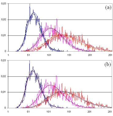
Figure 2: Histograms of (a) {SMSE(MoLC) - SMSE(SISE)} and (b)
{SMSE(MoLC) - SMSE(ML)} collected over 1000 independent samples of size N = 1000 with random configurations of parameters (ν, κ, σ).
The sampling and the respective estimation procedures were rerun 10 times and Table 2 presents the averages and the mean square errors (MSE) of the obtained estimates (compared to the true parameter values) over the performed 10 runs. Overall, MoLC estimates provided very competitive results that can in some cases be further refined by ML approach. Analyzing the SISE approach we can state the comparable accuracy of results as reported by MoLC. In or-der to further compare the performance of the estimation approaches we bring attention to several critical issues: first, the applicability, second, the sensitiv-ity of the estimators while operating with small sample sizes, and finally their computational complexity. We have always observed the ML convergence (NR procedure) initialized via MoLC which confirms the good MoLC accuracy in light of the generally unreliable behavior of ML approach to GΓD [25, 3]. It is worth noticing that the resulting two stage MoLC+ML approach constitutes a consistent estimator since both components have this property [2]. MoLC estimates demonstrated good competitive performance on small samples which became less pronounced with large sample sizes, especially as compared to ML which is largely known to be the best performing large sample estimator [30]. Fi-nally we can state the best computational performance demonstrated by MoLC, and especially so on larger sample sizes since this estimator does not involve it-erative sample statistics reestimation: This is demonstrated in th last column of Table 2 where we report the average computational times obtained on a Dual-core 1.83GHz, 2Gb RAM, WinXP system for the considered estimators on the sample size N = 5000. Further still, the polygamma and inverse polygamma functions numerical estimations involved in MoLC are fast and stable given the regular behavior of both functions.
We now comment on some large MSEs observed during the estimation pro-cess (see Table 2). We feel that it does not purely owe to the small sample sizes involved, but also reflects an inherent feature of the GΓD parameter estima-tion. More specifically, as has been observed in [24, 27], the GΓD pdf family is flexible to the point where substantially different parameter configurations can bring to close pdf shapes which renders the small sample parameter estimation procedure critically sensitive. To address this problem we estimate the obtained Kolmogorov-Smirnov (KS) distances
KS = max
x>0
¯¯
¯F (x) − F∗(x)¯¯¯
where F and F∗ are the estimated and the true GΓD cumulative distribution
functions, respectively. This distance represents one of the classical statistical tools to characterize the divergence between random variables [22]. Indeed, the values of KS distance allow to appreciate the accuracy of pdf estimation as a function, see Table 2. To present consistent results the obtained estimates have been averaged out over 10 runs.
To further evaluate the comparative performance of MoLC, we report the sample-based MSE (SMSE) estimation accuracy comparison generalizing the Nakagami pdf estimation analysis performed in [5]. More specifically, on 1000
independent samples{xi} of size N = 1000 each for the three considered
meth-ods we have calculated
SMSE = 1 N N ∑ i=1 ¯¯ ¯p(xi)− p∗(xi)¯¯¯ 2
where p and p∗ are the estimated and the true GΓD pdfs, respectively, and
constructed the histograms of {SMSE(MoLC)-SMSE(SISE)} (Fig. 2(a)) and
{SMSE(MoLC)-SMSE(ML)} (Fig. 2(b)). For each sample, the scale parameter
was fixed to σ = 1 and the shape parameters ν and κ were chosen randomly (uni-formly on [0.5, 50]). The analysis of the histograms (their bias to the negative side) reports slightly lower level of variances (in the form of SMSEs) achieved by MoLC.
The performed synthetic data experiments suggest MoLC to be a compet-itive alternative to ML and MoM whose principle advantages are the fast and stable computational procedure and the absence of initialization problem.
6.2
K distribution
Here we examine the applicability of MoLC parameter estimation strategy to the 3-parameter K-law distribution, which has been shown to represent the statis-tics of scattered signals at a diverse set of scales extending to both radar and sonar imagery [12], as well as some further applications (see, e.g., [6]). The pure ML strategy cannot be applied directly to this distribution since the derivative
of the modified Bessel function of the second kind Kν with respect to its index
does not allow an analytical expression. The Expectation-Maximization approx-imative iterative approach was used to address this problem in [31] and reported acceptable results for large sample sizes at the price of a heavy computational complexity. Similar conclusions were obtained with the other ML-approximation methods, for more details see [6]. Therefore, in most real applications with not excessively large size samples available and when the computational complexity is critical the MoM approaches might be preferable [6, 32]. These techniques, however, suffer from a nonzero probability that the moment equations are not invertible [6]: This occurs when the randomness inherent in the sample moments results in a moment ratio greater than the maximum theoretical value, which corresponds to a Rayleigh-distributed envelope. That means that for some sam-ples the MoM approach turns out to be inapplicable to the K distribution. As discussed in Section 5, MoLC approach is also restricted to samples that comply with (8), however, contrary to MoM, the respective applicability conditions are explicitly formulated in (8).
We present the comparison of the MoLC technique with the method of frac-tional moments (fMoM) that suffers from the same limitations as MoM (being its generalization) but demonstrates lower variances than MoM [32]. We con-sider the comparison with ML-based techniques for K-law outside of the scope of this study since we experimentally analyze foremost the small sample estimation performance, which is critically weak for ML-approaches to K [6]. In Table 3 the results of MoLC and fMoM parameter estimation for K-law with several pa-rameter configurations are presented. K-distributed samples were obtained via inverse transform sampling thanks to K-law representation as a product of two independent gamma-distributed random variables with parameters (1, L) and (µ, M ) [12]. As with GΓD, three sample sizes were considered and for each size the estimation process was rerun 10 times. Table 3 presents the average (over 10) estimates and the MSE between the estimates and the true parameter values.
For this comparison the samples for which either MoLC or fMoM failed to be applicable were not considered in this study. To analyze more the severeness of the applicability limitation given by (8) we generated 1000 K-distributed
Table 3: Average ( ¯L, ¯M ) and MSE ( ˆL− L∗, ˆM− M∗) of the K-law (with µ∗=
100, L∗, M∗) parameter estimates over 10 independently generated samples
obtained by MoLC and fMoM (ν =−0.75) for samples of sizes 250, 1000 and
5000
(L∗, M∗) (2, 10) (1, 20)
Sample Method Average MSE Average MSE
N = 250 MoLC (2.21, 11.26) (0.18, 2.17) (1.23, 18.81) (0.18, 3.21) fMoM (2.15, 7.92) (0.11, 2.31) (0.82, 18.21) (0.21, 3.54) N = 1000 MoLC (2.11, 9.41) (0.09, 1.57) (0.88, 21.12) (0.09, 2.32) fMoM (1.75, 9.40) (0.10, 1.87) (1.13, 18.92) (0.11, 2.71) N = 5000 MoLC (2.04, 9.90) (0.02, 1.13) (1.09, 20.51) (0.02, 1.44) fMoM (1.98, 11.12) (0.01, 1.10) (1.06, 19.39) (0.02, 1.62)
Table 4: GΓD parameter estimates on the ultrasound image on training sets of size N with obtained KS distances and classification accuracies
N Class 1 (black) Class 2 (white)
(ˆν, ˆκ, ˆσ) KS Acc (ˆν, ˆκ, ˆσ) KS Acc 1862 (0.84, 35.59, 2.86) 0.044 97.91% (3.08, 2.71, 87.39) 0.056 67.08% 912 (1.25, 25.71, 3.99) 0.044 97.70% (2.81, 3.06, 77.72) 0.060 68.13% 446 (0.91, 39.47, 1.88) 0.039 97.64% (1.55, 4.21, 66.04) 0.075 68.55% 218 (1.07, 38.74, 2.15) 0.041 97.41% (1.60, 4.04, 68.84) 0.070 69.07% 107 (2.72, 41.12, 1.44) 0.048 96.88% (0.97, 5.42, 61.35) 0.087 67.78%
samples of size N = 1000 each and concluded that MoLC approach failed (8)
in t1= 172 and fMoM was not applicable in t2= 154 cases. That suggests that
MoLC is considerably restrictive as applied to K law, which was experimentally observed in [4], and does not solve the problem of standard MoM applicability. For the reason of restricted applicability of both MoLC and fMoM the MSE comparison similar to the one presented in Fig. 2 is not feasible.
This study together with the conclusions obtained in [8] suggest the similar level of accuracy of MoLC and fMoM, with, however, an extra parameter to estimate for fMoM - the order of the lowest order moment employed ν. Further-more, both methods suffer from occasional inapplicability and, as such, some other more computationally intensive, yet universally applicable K parameter estimation approaches [6] might be preferable.
(a) Ultrasound image (b) Ground truth
(c) Result with N = 1862 (d) Result with N = 218
Figure 3: (a) Ultrasound image of gallbladder (with learning areas in
rect-angles), 250× 300 pixels, (b) nonexhaustive ground truth map (white, black
-mapped areas, grey tones - no ground truth) and GΓD-based supervised classi-fication results obtained with training samples of sizes: (c) N = 1862 and (d)
Figure 4: Plots of MoLC-based estimates for the ultrasound image obtained with the GΓD model: normalized histograms of the two considered classes and pdf estimates’ plots obtained with samples of sizes N = 1862 and N = 218.
(a) SAR image (b) Ground truth (c) GΓD with N = 912
(d) GΓD with N = 218 (e) K-root with N = 912
Figure 5: (a) SAR image of flooded area (with learning areas in rectangles)
of Piemonte, Italy (COSMO-SkyMed sensor, ©ASI), 1000× 1000 pixels, (b)
non-exhaustive ground truth map (white, black, grey - mapped areas, the rest - no ground truth) and supervised classification results obtained with: (c) GΓD model on N = 912 samples, (d) GΓD model on N = 218 samples and (e) K-root model on N = 912 samples.
Figure 6: Plots of MoLC-based estimates for the Piemonte image obtained
with (a) GΓD model (N1= 1862 and N2 = 218) and (b) K-root model (N1=
1862 and N2 = 912). Each graph contains normalized histograms of the three
considered classes and pdf estimates’ plots obtained with samples of two different sizes.
7
Real-data experiments
In this section we analyze the performance of the MoLC estimator applied to real-data. We notice that comparative performance of MoLC with alternative parameter estimation approaches for most of the pdf families in Table 1 in ap-plication to real imagery, and notably for SAR, has been previously tested: for GΓD in [17], Nakagami and Fisher models in [5, 19], GGR in [4], heavy-tailed Rayleigh in [10]. Further relevant MoLC-based mixture estimation experimental results were obtained for SAR pdf modeling in [16], and for SAR image classifi-cation in [23]. Therefore, in this section we concentrate on MoLC performance as a function of sample size which we will demonstrate for the GΓD and K families of distribution. The similar study has been performed previously for GGR and reported stable results in terms of correlation coefficient [4].
T able 5: GΓD and K -ro ot parameter estimates on the Piemon te image on training sets of size N with obtained KS distances and classification accuracies Class 1 (blac k) Class 2 (grey) Class 3 (white) GΓD N ( ˆν , ˆκ, ˆσ ) KS Acc ( ˆν , ˆκ, ˆσ ) KS Acc ( ˆν , ˆκ, ˆσ ) KS Acc 1862 (1.02, 12.60, 5.67) 0.021 96.19% (1.21, 7.29, 28.55) 0.019 93.79% (1.16, 7.47, 33.02) 0.018 95.97% 912 (1.01, 11.76, 4.81) 0.026 96.07% (1.07, 9.36, 23.32) 0.034 94.24% (1.25, 5.25, 40.64) 0.022 96.48% 446 (1.28, 5.22, 14.24) 0.032 96.16% (1.29, 5.61, 39.19) 0.035 94.82% (1.42, 3.38, 47.90) 0.026 97.24% 218 (1.39, 4.30, 21.19) 0.048 95.58% (1.34, 4.88, 45.20) 0.029 95.24% (1.37, 3.64, 50.52) 0.041 97.33% K -ro ot N ( ˆµ, ˆ L, ˆ M) KS Acc ( ˆµ, ˆ L, ˆ M) KS Acc ( ˆµ, ˆ L, ˆ M) KS Acc 1862 (66.63, 5.93, 8.79) 0.022 96.17% (113.11, 4.80, 23.13) 0.020 93.77% (149.22, 4.48, 16.39) 0.026 95.77% 912 (66.12, 4.91, 10.03) 0.025 96.08% (113.07 4.85, 21.61) 0.029 93.89% (146.23, 3.86, 26.36) 0.028 96.51%
In this report, we consider two types of speckled imagery: medical ultrasound and remote sensing SAR, both in application to supervised image classification. To analyze the small sample performance of MoLC we start with training
sam-ples of N ≈ 2000 observations and gradually reduce its size down to N ≈ 200.
First we demonstrate the fit of MoLC estimated pdfs with the normalized his-tograms and employ the Kolmogorov-Smirnov distance (KS) to quantify the obtained goodness-of-fit. Second, we analyze the MoLC performance in appli-cation to supervised image classifiappli-cation as a function of training sample size. To this end we construct classification maps and quantify the obtained accuracy by referring to non-exhaustive ground truth maps. The classification maps are obtained following a likelihood based approach [1] and, therefore, rely directly on the estimated pdf models and serve to characterize the estimation accuracy. In order to take into consideration spatial context in the image and improve the robustness of classification with respect to speckle [13] we employ the Markov random field approach via 2-nd order Potts model, see [1, 23]. The weight coef-ficient for this single parametric model is set manually based on trial and error method. To minimize the energy of the resulting Gibbs distribution we employ the graph cut approach based on expansion-moves [33, 34, 35].
First we investigate an ultrasound image of gallbladder, see Fig. 3(a). The considered classification is binary and the available non-exhaustive ground truth is presented in Fig. 3(b). The training areas come from the same image, see rectangles in Fig. 3(a) indicating the areas of size N = 1862. The first impor-tant observation is that for this image both, the Fisher and, consequently, the
K model (see Section 5), turned to be inapplicable, same for the fMoM method
of K. On the other hand, GΓD model was applicable for all sample sizes. The normalized histograms for both classes along with GΓD pdf estimates’ plots on
samples of sizes N1 = 1862 and N4 = 218 are presented in Fig. 4. The
cor-responding parameter estimates with the obtained KS distances are presented
in Table 4 for sample sizes from the initial N1 = 1862 to N5 = 107 (at each
step, the learning areas were reduced by taking out∼ 50% of randomly chosen
pixels). It is immediate, that the quality of pdf estimation both qualitatively (pdf plots) and quantitatively (KS) remains on the same level going from sample
size N1to N4, whereas the actual parameter estimates’ values demonstrate some
fluctuations. On the last step presented in Table 4 (N = 107) the estimation accuracy dropped significantly due to critically small sample size. Fig. 3(c)-(d) present the classification maps obtained with MoLC estimates based on samples
of sizes N1 and N4, respectively. The visual analysis reports negligible
classi-fication difference, and this observation is further confirmed by percentage of correct classification reported in Table 4.
The second set of experiments is conducted on a SAR image obtained by the COSMO-SkyMed satellite system in the Stripmap mode over an agricultural area in Piemonte, Italy (single-look, HH-polarized, 2.5-m ground resolution, 2008), see Fig. 5(a). On this image we investigate the performance of MoLC applied to the GΓD and K models to the supervised three class classification with the manually prepared non-exhaustive ground truth presented in Fig. 5(b). Since the considered image is in the amplitude domain, the K model is replaced by its amplitude equivalent K-root. As with the ultrasound image we start with learning areas of size N = 1862 pixels (delimited with rectangles in Fig. 5(a)) and go down to N = 218. We first notice that the GΓD model is applicable to all considered sample sizes, whereas reiterating the learning area subsampling
for the K-root model we persistently observed its inapplicability (i.e. failure to comply with restriction (9)) starting from sample size N = 446, notably so for class 3. We further report that the Fisher model failed altogether starting from the initial sample size to deal with classes 2 and 3 that reported sample values
of ˜k2and ˜k3outside of applicability region given by (10). The attempts to solve
this problem by changing the location of learning areas did not report success. Plots of pdf estimates obtained for the considered target classes with GΓD and
K-root models are presented in Fig. 6, classification maps in Fig. 5(c)-(e), and
numerical estimation and classification results are summarized in Table 5. From these experimental results we conclude that the estimation accuracy of MoLC demonstrates acceptably stable behavior with respect to small sample, and especially for classification purposes, where not the parameter values but rather the histogram fit is of importance. On the other hand the applicability restrictions of MoLC for some pdf families, including Fisher and K distributions, might be critical and need to be constantly verified.
8
Conclusions
In this report we have addressed the problem of pdf parameter estimation by means of the MoLC approach. This recently developed estimator found a wide range of applications, notably for SAR image processing, where the multiplica-tive nature of the underlying Mellin integral transform allows MoLC to accu-rately describe advanced texture-speckle statistical product models. We have demonstrated an important statistical property of strong consistency of MoLC estimates for a representative selection of pdf models for which the classical parameter estimators, such as ML and MoM, experience difficulties. For several distribution families, we then derived easy-to-check explicit analytical condi-tions of MoLC estimator applicability to a given sample to provide a complete picture of MoLC properties. The conducted synthetic-data experiments demon-strated a competitive accuracy of MoLC estimates and a reliable behavior of this estimator for small samples which is a critical issue in applications. Finally, we performed real-data image processing experiments to the problem of supervised classification applied to medical ultrasound and remote sensing SAR imagery. These experiments confirmed the stability of MoLC estimator with respect to sample size and at the same time illuminated the critical side of MoLC given by applicability restrictions.
Based on the Mellin transform, the MoLC approach can be considered as an alternative to MoM that is both more robust to outliers and in some important cases demonstrates better variance properties. On the other hand the issue of MoLC estimator applicability for a specific distribution to a given sample is critical and need to be constantly verified. Applied to a selection of pdf families MoLC enabled to obtain more feasible systems of equations and demonstrated better small sample properties as compared to MoM in situations when the ML approach is not directly applicable. Finally, the analysis performed in this report suggests MoLC, even with its restrictions, to be a valid estimator can-didate in case of multiplicative pdf models or when the classical ML and MoM methodologies fail to provide well-established estimators.
Acknowledgments
The first author was funded as a postdoc by the Institut National de Recherche en Informatique et en Automatique, France (INRIA). The authors would like to thank the Italian Space Agency for providing the COSMO-SkyMed (CSK®) image of Piemonte (COSMO-SkyMed Product - ©ASI - Agenzia Spaziale Ital-iana - 2008. All Rights Reserved).
Appendices
A
Proofs of theorems 1-3
Proof of Theorem 1. Let{xn}∞n=1 be a sequence of independent identically
distributed observations xn∼ pξ∗(·). To prove the consistency of MoLC, where
each estimate ˆξn is based on n first observations from {xn}∞n=1, we need to
demonstrate the convergence in probability of ˆξn to ξ∗ as n→ ∞, i.e.:
lim n→∞P { ||ˆξn− ξ∗||∞< ε } = 1
for any ε > 0, where by||v||∞= max
i=1,...,d|vi| we denote the uniform norm of an
d-dimensional vector v.
Define Θ : Ξ→ RM as a mapping of parameter vector ξ into log-cumulants
k. Thus, the vector of log-cumulants k∗ corresponding to the true parameter
values ξ∗may be found as k∗= Θ(ξ∗).
It is well known that the sample estimates of the log-cumulants ˆksn, s∈ N,
defined by the right hand side of (5) are consistent estimates of the central moments of the random variable ln X (see [22]).
If we employ now the continuity of mapping Θ−1 at ˆk∗, we obtain the
fol-lowing: for any ε > 0, there exists δε > 0 such that if ||ˆk − k∗||∞ < δε and
ˆ
k∈ Θ(Ξ), then ||Θ−1(ˆk)− ξ∗||∞< ε. Therefore, if by ||v|| = (v2
1+ . . . + v2n)1/2
we denote the Euclidean norm of the vector v, then from||ˆkn− k∗|| < δεfollows
||ˆξn− ξ∗||∞< ε or, in other words,
P{||ˆξn− ξ∗||∞< ε} > P{||ˆkn− k∗|| < δε}. (11)
By applying the Markov and Cauchy-Schwarz inequalities [22], we obtain:
P{||ˆkn− k∗|| < δε} > 1 − E{||ˆkn− k∗||} δε > 1 − ( E{||ˆkn− k∗||2} )1/2 δε . Therefore, P{||ˆξn−ξ∗||∞< ε} > 1− ( E{||ˆkn− k∗||2} )1/2 δε = 1− ( E{∑M s=1|ˆksn− k∗s|2} )1/2 δε = = 1− ( E{∑M s=1 [ ˆ ksn− ks∗− O (1 n )]2 + O(n12 )})1/2 δε .
We now take into account that [30]
Eˆksn= k∗s+ O ( 1 n ) and, hence, E[ˆksn− k∗ s− O ( 1 n )]2 =E [ ˆ ksn− Eˆksn ]2 =Dˆksn