HAL Id: hal-01584206
https://hal.archives-ouvertes.fr/hal-01584206
Submitted on 17 Sep 2020
HAL is a multi-disciplinary open access
archive for the deposit and dissemination of
sci-entific research documents, whether they are
pub-lished or not. The documents may come from
teaching and research institutions in France or
abroad, or from public or private research centers.
L’archive ouverte pluridisciplinaire HAL, est
destinée au dépôt et à la diffusion de documents
scientifiques de niveau recherche, publiés ou non,
émanant des établissements d’enseignement et de
recherche français ou étrangers, des laboratoires
publics ou privés.
Enhanced methane emissions from tropical wetlands
during the 2011 La Niña
Sudhanshu Pandey, Sander Houweling, Maarten Krol, Ilse Aben, Guillaume
Monteil, Narcisa Nechita-Banda, Edward J. Dlugokencky, Rob Detmers, Otto
Hasekamp, Xiyan Xu, et al.
To cite this version:
Sudhanshu Pandey, Sander Houweling, Maarten Krol, Ilse Aben, Guillaume Monteil, et al.. Enhanced
methane emissions from tropical wetlands during the 2011 La Niña. Scientific Reports, Nature
Pub-lishing Group, 2017, 7 (1), pp.45759. �10.1038/srep45759�. �hal-01584206�
Enhanced methane emissions from
tropical wetlands during the 2011
La Niña
Sudhanshu Pandey
1,2, Sander Houweling
1,2, Maarten Krol
1,2,3, Ilse Aben
2, Guillaume Monteil
4,
Narcisa Nechita-Banda
2, Edward J. Dlugokencky
5, Rob Detmers
2, Otto Hasekamp
2,
Xiyan Xu
6,7, William J. Riley
6, Benjamin Poulter
8, Zhen Zhang
9, Kyle C. McDonald
10,
James W. C. White
11, Philippe Bousquet
12& Thomas Röckmann
1Year-to-year variations in the atmospheric methane (CH4) growth rate show significant correlation
with climatic drivers. The second half of 2010 and the first half of 2011 experienced the strongest La Niña since the early 1980s, when global surface networks started monitoring atmospheric CH4 mole
fractions. We use these surface measurements, retrievals of column-averaged CH4 mole fractions from
GOSAT, new wetland inundation estimates, and atmospheric δ13C-CH
4 measurements to estimate
the impact of this strong La Niña on the global atmospheric CH4 budget. By performing atmospheric
inversions, we find evidence of an increase in tropical CH4 emissions of ∼6–9 TgCH4 yr−1 during this
event. Stable isotope data suggest that biogenic sources are the cause of this emission increase. We find a simultaneous expansion of wetland area, driven by the excess precipitation over the Tropical continents during the La Niña. Two process-based wetland models predict increases in wetland area consistent with observationally-constrained values, but substantially smaller per-area CH4 emissions,
highlighting the need for improvements in such models. Overall, tropical wetland emissions during the strong La Niña were at least by 5% larger than the long-term mean.
CH4 is the second most important anthropogenic greenhouse gas after CO2, accounting for 20% of direct
anthro-pogenic radiative forcing1. CH
4 contributes strongly to anthropogenic climate change, directly through its
radia-tive forcing as well as indirectly through impacts on atmospheric chemistry2. With a relatively short atmospheric
lifetime of ∼ 9 years, CH4 is a primary target for global warming mitigation strategies3. Over the past decades,
the atmospheric CH4 growth rate has been highly variable3–7, including an approximate stabilization from 1999
to 2006 followed by a renewed growth since 20078. Among a range of explanations that were proposed, some
studies have suggested that more than 70% of the interannual variations of CH4 can be explained by wetland CH4
emissions9,10.
Wetland CH4 emissions are highly sensitive to soil temperature and moisture11. Paleo records and studies of
contemporary CH4 suggest a strong positive feedback of wetlands to global warming through CH4 emissions12,13.
Proper quantification of this feedback is important for accurate future climate projections. Therefore, it is crucial to better understand the sensitivity of wetland CH4 emissions to changes in climatic parameters. The El Niño
Southern Oscillation (ENSO) is a major mode of variability of global precipitation and temperature, comprising alternating El Niño and La Niña phases14. Hodson et al.15 estimated the influence of precipitation and
tempera-ture change, driven by ENSO, on wetland CH4 emissions using a process-based wetland model. They found that 1Institute of Marine and Atmospheric Research Utrecht (IMAU), Utrecht, The Netherlands. 2SRON Netherlands
institute for Space Research, Utrecht, The Netherlands. 3Department of Meteorology and Air Quality (MAQ),
Wageningen University and Research Centre, Wageningen The Netherlands. 4Department of Physical Geography
and Ecosystem Science, Lund University, Lund, Sweden. 5NOAA Earth System Research Laboratory, Boulder,
Colorado, USA. 6Earth Sciences Division, Lawrence Berkeley National Laboratory, Berkeley, California, USA. 7CAS
Key Laboratory of Regional Climate-Environment for Temperate East Asia, Institute of Atmospheric Physics, Beijing, China. 8Institute on Ecosystems and Department of Ecology, Montana State University, Bozeman, USA. 9Swiss
Federal Research Institute WSL, Birmensdorf, Switzerland. 10City College of New York, City University of New York,
New York, NY, USA. 11Institute of Arctic and Alpine Research, Boulder, CO, USA. 12Laboratoire des Sciences du
Climatet de l’Environnement (LSCE), Gif-sur-Yvette, France. Correspondence and requests for materials should be addressed to S.P. (email: [email protected])
Received: 18 October 2016 Accepted: 03 March 2017 Published: 10 April 2017
www.nature.com/scientificreports/
a large fraction of CH4 variability is correlated with ENSO, with higher tropical wetland CH4 emission during La
Niña periods. However, this pattern has not been verified until now by atmospheric CH4 measurements during
a La Niña. Furthermore, La Niña periods have received less attention in studies of the atmospheric CH4 budget
than El Niño, since continued warming likely favors neutral or El Niño conditions16.
The La Niño of 2011 (LN11 hereafter) was the strongest since 1980 (see Fig. 1a) and offers the possibility to investigate the response of the atmospheric CH4 budget to La Niña conditions. In this study, we investigate this
response by combining different measurement dataset and model simulations. A brief overview of them is given in the next section.
Method and Data
Atmospheric CH4 measurements are available during the 2011 La Niña period from ground-based networks
(NOAA-ESRL, CSIRO), and space (GOSAT, SCIAMACHY). The Greenhouse Gases Observing Satellite (GOSAT) has been measuring spectra for retrieval of the column average mole fraction of CH4 (XCH4) since June
200917. Onboard GOSAT is the Thermal And Near infrared Sensor for carbon Observation-Fourier Transform
Spectrometer (TANSO-FTS), from which XCH4 is obtained with high sensitivity to the lower troposphere, and
hence, to surface emissions18. We analyze the interannual variability in GOSAT full-physics (FP) XCH
4, obtained
using the RemoteC algorithm19, and ground-based CH
4 flask-air measurements. Supplementary Material (SM)
Section 9 further explains the FP retrieval method and justifies our choice of FP XCH4 over XCH4 derived from
other retrieval algorithms.
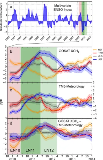
Figure 1. (a) Multivariate ENSO index (MEI53). The strong La Niña of 2011 (LN11) is shaded in dark green.
The preceding El Niño of 2010 (EN10) and succeeding weak La Niña of 2012 (LN12) are shaded in lighter red and green colors, respectively. (b,c,d) Detrended and smoothened XCH4 integrated over the large regions: (b)
GOSAT FP XCH4, (c) TM5-Meteorology XCH4—that is, XCH4 variability due to meteorological changes (TM5
is run with annually repeating emissions). (d) GOSAT FP XCH4 corrected for the influence of meteorology
(the difference between b and c). The light shaded regions represent the ± 1σ uncertainty of the respective time series. NET, SET, TRO, and GLO are abbreviation of Northern Extra Tropics, Southern Extra Tropics, Tropics and Globe, respectively.
In addition to the surface emissions, changes in atmospheric transport can cause interannual variability in CH420. Large-scale transport patterns, including the strength of inter-hemispheric exchange and atmospheric
temperature are influenced by ENSO3,21–23. To quantify the contribution of these meteorological parameters,
we ran the Tracer Transport Model version 5 (TM524) repeating surface emissions of 2008 for every year in
2009–2015. This simulation is referred to as TM5-Meteorology from hereon (see SM Section 1). To quantify the contribution of the surface emissions to XCH4 variability, we look at the difference between GOSAT FP XCH4 and
XCH4 sampled from TM5-Meteorology.
Atmospheric inverse modeling systems are well established tools to convert atmospheric CH4 measurements
into surface emissions25,26. We use the TM5-4DVAR (TM5-variational data assimilation system27) in combination
with GOSAT FP XCH4, and surface measurements from NOAA-ESRL3 and CSIRO28 to optimize surface CH4
emissions. Note that the inverse model makes use of actual meteorological fields from the ECMWF ERA-interim reanalysis to account for variability in the atmospheric transport of CH4. Earlier studies have established the link
between biomass burning CH4 emissions and ENSO29. To exclude the influence of biomass burning, fire related
CH4 emissions from the Global Fire Emissions Database version 4s (GFED4s) inventory have been subtracted
from the TM5-4DVAR emissions.
The origin of an atmospheric CH4 anomaly can be identified using CH4 stable isotope measurements. We
look at measurements of 13C/12C in CH
4 (expressed in δ-notation as δ13C-CH4) analyzed by INSTAAR in samples
from the NOAA-ESRL (ref. 30, see Fig. 2b). δ13C-CH
4 of atmospheric CH4 (global average in 2009= − 47.14‰) is
controlled by the relative contribution from different source types with distinct isotopic signatures. The mean iso-topic signatures of the biogenic category is ∼ − 60‰ (includes wetlands, agriculture, waste), for the thermogenic category it is ∼ − 37‰ (includes fossil-fuels) and for pyrogenic category it is ∼ − 22‰ (includes biomass burn-ing)31. To account for impact of meteorological variability on δ13C-CH
4, a meteorology simulation of δ13C-CH4
was performed using TM532.
To identify factors which might have altered the wetland emissions, we look at the variability in land precipi-tation and temperature data in CRU-TS version 3.23 (Climatic Research Unit-time series33). We also analyze CH
4
emission and surface inundation extent from two process-based wetland models: LPJ-wsl15,34 and CLM4.535,36.
Additionally, we derive an independent estimate of inundation extent from remotely sensed Surface WAter Microwave Product Series (SWAMPs37).
The primary sink of CH4 is the reaction with OH in the troposphere (∼ 454–617 TgCH4 yr−12), and
inter-annual variations in OH can also contribute to the observed CH4 variability. Tropospheric OH concentrations
are influenced by many factors, including temperature, water vapor, O3, NOx, CH4, CO, and the overhead
strat-ospheric ozone column38. The TM5-4DVAR inversions performed in this study make use of OH fields from ref.
39, which vary seasonally, but are the same each year. To investigate possible variations caused by the OH sink, we analyze posterior CH4 emissions of LMDz-PYVAR-SACS inversion40–42. In this inversion, the OH fields were
optimized simultaneously using methyl chloroform (MCF) measurements (see SM Section 1.3).
Data Analysis.
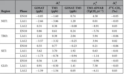
The above mentioned measurements and model outputs have been analyzed by taking their monthly averages and integrating them over three zones over the globe (GLO) : Tropics (TRO: 30°S to 30°N), Northern Extra Tropics (NET: 30°N to 90°N), Southern Extra Tropics (SET: 90°S to 30°S). The time series of these monthly averages have been detrended and smoothened using a 12 month running mean. The resultingFigure 2. (a) Detrended and smoothened CH4 surface emissions estimates from TM5-4DVAR for the same
regions as in Fig. 1. The variability of GFED4s biomass burning emissions has been subtracted. (b) δ13C-CH 4
measurements54 corrected for the influence of transport using a meteorology-only TM5 simulation of δ13C-CH
www.nature.com/scientificreports/
time series of GOSAT FP XCH4 from this method is less influenced by systematic errors, which often affect the
satellite retrievals9,43,44.
Further, based on the Multivariate ENSO index (MEI) we define three periods: 1) La Niña in 2011 as LN11; 2) The preceding El Niño of 2010 as EN10; 3) succeeding weak La Niña of 2012 as LN12 (see Fig. 1a). Time series of measurements and model outputs are analyzed during these periods using the following parameters:
1. ∆rq: Defined as the change of a quantity q in region r during an ENSO phase.
2. µrq: Defined as the mean of a quantity q in region r during an ENSO phase.
Table 1 summarizes ∆rq or µ
rq of time series shown in Figs 1 and 2.
Results and Disscussion
GOSAT observations.
Figure 1b shows detrended and smoothened time series of GOSAT FP XCH4. DuringLN11, SET and TRO have increasing XCH4 (∆XCHSET 4 = 5.6ppb and ∆XCHTRO4 = 2.4) contrasted by a decrease in NET
(∆XCH
NET4 = − 2.7 ppb). During LN12, the opposite trends are found: XCH4 gradually reduced in SET and TRO and
increased in NET.
Figure 1c shows the results of TM5-Meteorology simulation. The modeled XCH4 decreases over NET and
increases over SET (∆XCH = .3 7
SET 4 ppb, ∆NETXCH4= − .3 9 ppb). These trends can be attributed to the faster
inter-hemispheric exchange during La Niña conditions, which transferred additional CH4 rich air from the
Northern Hemisphere to the Southern Hemisphere. Francey et al.21 found the strongest inter-hemispheric
trans-port of CH4 during LN11 since 1990. Previous studies have reported such enhancement in inter-hemispheric
transport, and consequent increase in CH4 in the Southern Hemisphere, during the La Niña of 2007–20083 and
198923. During LN12, the strength of anomalies over both regions weakens as inter-hemispheric exchange returns
to its normal strength. Modeled XCH4 over TRO show less variation during LN11. During LN12, the modeled
XCH4 (∆XCHTRO4= − .3 3 ppb) explains a major fraction of GOSAT XCH4 (∆TROXCH4= − .3 6 ppb) variability. It is
noteworthy that OH concentrations are not affected in our meteorology simulation as TM5 uses OH fields from Spivakovsky et al.39. Eventhough these fields don’t vary interannually, temperature variations can still cause
vari-ability in the atmospheric CH4 sink, as the rate constant for reaction with OH is temperature dependent45.
Figure 1d shows the GOSAT FP XCH4 after correction for variations in atmospheric transport using the
TM5-Meteorology simulation, and indicates the fraction of CH4 variability that can be attributed to variability in
CH4 sources and sinks. An analogous plot showing surface flask-air measurements is given in the SM section 4
and shows similar patterns. During LN11, the largest transport-corrected ∆XCH4 is seen in TRO (∆XCH = .2 0 TRO4
ppb), pointing to higher CH4 emissions from the tropical continents. As SET does not have large CH4 surface
emissions, it is caused most likely by transport from TRO. This means the transport-corrected anomaly of TRO is transferred to SET.
Emissions and source attribution.
Detrended and smoothened time series of the posterior TM5-4DVAR emissions are shown in Fig. 2a. The CH4 emissions over TRO show a positive anomaly during LN11(µTROemission= .5 9 TgCH
4 yr−1). µTROemission is higher by 11.7 TgCH4 yr−1 in LN11 than in the preceding EN10
(µTROemission= − .5 8 TgCH4 yr−1). This can be due to higher CH4 emissions from tropical wetlands during the La
Niña, as suggested by ref. 15. During LN12, the CH4 emission enhancement over TRO is weaker (µTROemission= .3 9 Region Phase ∆rq µrq ∆rq GOSAT (ppb) (ppb)TM5 GOSAT-TM5(ppb) TM5-4DVAR(TgCH4 yr−1) δ13C-CH4 (‰) NET: EN10 − 0.85 − 1.60 0.74 4.58 − 0.05 LA11 − 2.66 − 3.86 1.20 0.01 − 0.03 LA12 0.31 0.38 − 0.08 − 8.91 0.03 TRO: EN10 0.86 0.61 0.24 − 5.76 0.01 LA11 2.42 0.38 2.04 5.94 − 0.06 LA12 − 3.57 − 3.32 − 0.25 3.94 0.02 SET: EN10 0.55 0.77 − 0.23 0.21 − 0.06 LA11 5.62 3.70 1.92 0.63 − 0.01 LA12 − 1.73 − 0.78 − 0.94 − 1.14 0.03 GLO: EN10 0.56 1.18 − 0.61 − 0.96 − 0.03 LA11 0.91 − 0.50 1.41 7.58 − 0.03 LA12 − 1.59 − 1.54 0.05 − 6.11 0.03
Table 1. ∆rq (i.e. the sum of the derivative) or µrq (i.e. mean) of the times series of quantity q, averaged over
region r, as shown in Figs 1 and 2 during different ENSO phases. Please note that the GOSAT and
TM5-4DVAR time series do not cover the whole EN10 period, as continuous GOSAT measurements are only available since June 2009, and the 12-month smoothing causes data points loss. Only δ13C-CH
4 values cover the
TgCH4 yr−1). NET has a sharp decrease in CH4 emissions during LN11 (∆NETemission= −13 TgCH4 yr−1), which
shifts the maximum of the global CH4 emission anomaly towards the beginning of LN11.
Detrended and smoothened time series of δ13C-CH
4 is shown in Fig. 2b. During LN11, δ13C-CH4 decreased
over each region. Over TRO, we observe a decrease of 0.06‰, which is a larger decrease than the GLO δ13C-CH 4
decrease by 0.03‰. An isotope mass balance calculation shows that if the increase in TRO CH4 emissions of 11.7
TgCH4 yr−1 (change from EN10 with µTROemission= − .5 8 TgCH4 yr−1 to LN11 with µTROemission= .5 9 TgCH4 yr−1), is
attributed to a biogenic source, it would cause a drop in δ13C-CH
4 of similar magnitude. This indicates that the
source of the LN11 CH4 anomaly in the Tropics is of biogenic origin. The increase of GLO δ13C-CH4 (≈ 0.03‰)
over LN12 can be explained by reduced biogenic emissions (µGLOemission(LN12) - µ
GLOemission(LN11) = ∼ − 14 TgCH4
yr−1) and increased biomass burning emissions (µ
GLOGFED4s (LN12) – µGLOGFED4s (LN11) = 2.2 TgCH4 yr−1) in
compar-ison to LN11.
Tropical Biomass burning is strongly influenced by ENSO46. Globally, GFED4s biomass burning CH 4
emis-sions indicate a decrease of 0.67 TgCH4 yr−1 from EN10 to LN11 (see SM Section 5). The effect of this change on
the isotopic composition is only − 0.003‰, thus much smaller than the observed trend. According to GFED4s, CH4 emissions from biomass burning over TRO during LN11 are close to average over the whole period
(µTROGFED4s = − 0.23 TgCH
4 yr−1). In LN12, these emissions were higher in NET and TRO (µTROGFED4s = 1.09 TgCH4
yr−1 and µ
NETGFED4s = 1.32 TgCH4 yr−1). This increase may be explained by higher fuel availability due to enhanced
biomass growth during the preceding LN11. Ref. 47 suggested a similar impact of Australian biomass burning on CO2 emissions.
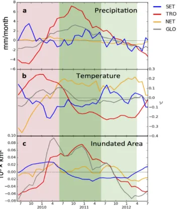
Figure 3a and b show monthly anomalies recorded in climate parameters. A significant redistribution of heat and precipitation is seen during the different phases of ENSO. µTROprecipitation was − 1.72, 4.90, and 0.64 mm during
EN10, LN11, and LN12, respectively. During LN11 the precipitation anomaly in TRO (and in GLO) was the highest since the onset of the 21st century (see SM Figure 10). Regions like Australia had six consecutive seasons of increased rainfall over the La Niña of 2011 and 201248. Higher temperatures were observed in NET during
LN11 (µNETtemperature = 0.18 °C), favoring increased biomass burning, for example, near Moscow during the summer
of 201049,50. Mean temperatures during LN11 (µ
TROtemperature = − 0.05 °C) were in between those during EN10
(µTROtemperature = 0.15 °C) and LN12 (µ
TROtemperature = − 0.22 °C).
An increase in total inundated area is observed in the remotely sensed SWAMPS data (see Fig. 3c). The total inundated area estimated by the wetland models LPJ-wsl and CLM4.5 also show a similar increase. However, these wetland models estimate a relatively weaker enhancement in CH4 emissions with µTROemission= .1 54 TgCH4
yr−1 for LPJ-wsl and µ = .2 38
TROemission TgCH4 yr−1 for CLM4.5 during LN11 (see SM Section 8).
To further investigate the relation between inversion-estimated CH4 emissions and potential climatic drivers, we
examine their correlation coefficients (R) [see SM Figure 11]. CH4 emission anomalies (as shown in
Figure 3. (a,b) Detrended and smoothened regionally averaged precipitation and temperature measurements
over land in CRU-TS version 3.23 (Climatic Research Unit-time series33). (c) Anomalies in the total inundated
www.nature.com/scientificreports/
Fig. 2a) correlate stronger with precipitation anomalies than with temperature anomalies (as shown in Fig. 3) in both NET Rprecipitation,emission= .0 86, Rtemperature,emission= − .0 52) and TRO (Rprecipitation,emission= .0 85,
= − .
Rtemperature,emission 0 62). This points to precipitation as the more important driver of the CH4 anomaly in TRO
during LN11, supported further by the correlation with inundated area (Rinundation,emission= .0 67). This is consistent with the findings of Bloom et al.51, who show that precipitation plays a more dominant role than temperature in
deter-mining anomalous CH4 variability in the Tropics.
To investigate possible variations caused by the OH sink, we analyzed optimized CH4 emissions from a
LMDz-PYVAR-SACS inversion, in which OH fields were also optimized. During LN11, the results of this inver-sion suggest µTROemission of 9.1 TgCH
4 yr−1, compared to TM5-4DVAR µTROemission of ∼ 6 TgCH4 yr−1 (see SM Section
6). The differences in interannual variations of the emission estimates of the two inversions are mainly caused by their different treatment of OH sink. Assuming that the MCF-optimized OH sink of LMDz-PYVAR-SACS is more accurate than TM5, the sink was stronger than normal during LN11 by ∼ 3 TgCH4 yr−1. This is consistent
with the hypothesis of an increased CH4 sink during La Niña and a weaker sink during El Niño52.
Conclusion
Our inversion results, supported by δ13C-CH
4 measurements, provide strong evidence of enhanced tropical
bio-genic CH4 emissions by ∼ 6–9 TgCH4 yr−1, during the La Niña of 2011. Wetlands were the likely cause of this
anomaly as a simultaneous increase in total inundated area is shown by remote sensing observations and hydro-logical models. The increase in inundated area was in response to La Niña induced increase in precipitation. 2011 experienced the strongest La Niña event in the past 4 decades as well as since the onset of modern atmospheric CH4 measurements. It is noteworthy that during this La Niña the increase in global CH4 mole fractions were not
as pronounced due to a simultaneous decrease in the CH4 emissions in the Northern Extra Tropics. Our analysis
presents the first evidence of the large-scale response of wetland CH4 emissions to ENSO variability using satellite
retrievals.
Data Availability
We use Level 2 SRFP XCH4 v2.3.7 GOSAT XCH4 retrievals that are publicly available from ESA’s Climate Change Initiative website (www.esa-ghg-cci.org/). NOAA CH4 and INSTAAR δ13C-CH4 measurements are freely avail-able from NOAA’s public ftp server (ftp://aftp.cmdl.noaa.gov/data). CSIRO CH4 measurements can be down-loaded from the WDCGG (World Data Centre for Green-house Gases) website. GFED4s CH4 emissions can be downloaded from http://daac.ornl.gov. CRU TS3.23). Precipitation and temperature data are held at British Atmospheric Data Centre, RAL, UK (http://badc.nerc.ac.uk/data/cru/). SWAMP wetlands fraction data can be downloaded from http://wetlands.jpl.nasa.gov after a short registration. CLM4.5 and LPJ-wsl CH4 emissions and wetlands fractions can be obtained by contacting William J. Riley and B. Poulter, respectively.
References
1. Myhre, G. et al. Anthropogenic and Natural Radiative Forcing. In Stocker, T. F. D., Qin, G.-K., Plattner, M., Tignor, S. K., Allen, J., Boschung, A., Nauels, Y., Xia, V. B. & (eds)]., P. M. (eds) Climate Change 2013: The Physical Science Basis. Contribution of Working
Group I to the Fifth Assessment Report of the Intergovernmental Panel on Climate Change, 659–740 (Cambridge University Press,
Cambridge, United Kingdom and New York, NY, USA, 2013).
2. Kirschke, S. et al. Three decades of global methane sources and sinks. Nature Geoscience 6, 813–823 (2013).
3. Dlugokencky, E. J. et al. Observational constraints on recent increases in the atmospheric CH4 burden. Geophysical Research Letters
36, L18803 (2009).
4. Heimann, M. Atmospheric science: Enigma of the recent methane budget. Nature 476, 157–158 (2011).
5. Kai, F. M., Tyler, S. C., Randerson, J. T. & Blake, D. R. Reduced methane growth rate explained by decreased Northern Hemisphere microbial sources. Nature 476, 194–7 (2011).
6. Aydin, M. et al. Recent decreases in fossil-fuel emissions of ethane and methane derived from firn air. Nature 476, 198–201 (2011). 7. Ferretti, D. F. et al. Unexpected changes to the global methane budget over the past 2000 years. Science (New York, N.Y.) 309, 1714–7
(2005).
8. Nisbet, E., Dlugokencky, E. J. & Bousquet, P. Methane on the Rise–Again. Science 343, 493–495 (2014).
9. Bousquet, P. et al. Contribution of anthropogenic and natural sources to atmospheric methane variability. Nature 443, 439–43 (2006).
10. Chen, Y. H. & Prinn, R. G. Estimation of atmospheric methane emissions between 1996 and 2001 using a three-dimensional global chemical transport model. Journal of Geophysical Research Atmospheres 111, 1–25 (2006).
11. Christensen, T. R. Factors controlling large scale variations in methane emissions from wetlands. Geophysical Research Letters 30, 10–13 (2003).
12. Nisbet, E. G. & Chappellaz, J. Shifting Gear, Quickly. Science 324, 477–478 (2009). 13. Petrenko, V. V. et al. 14CH
4 Measurements in Greenland Ice: Investigating Last Glacial Termination CH4 Sources. Science 324,
506–508 (2009).
14. Walker, G. & Bliss, E. World weather V. Memoirs of the Royal Meteorological Society 4, 53–84 (1932).
15. Hodson, E. L., Poulter, B., Zimmermann, N. E., Prigent, C. & Kaplan, J. O. The El Niño-Southern Oscillation and wetland methane interannual variability. Geophysical Research Letters 38, 3–6 (2011).
16. Cai, W. et al. Increasing frequency of extreme El Niño events due to greenhouse warming. Nature Climate Change 5, 1–6 (2014). 17. Yokota, T. et al. Global Concentrations of CO2 and CH4 Retrieved from GOSAT: First Preliminary Results. SOLA 5, 160–163 (2009).
18. Kuze, A., Suto, H., Nakajima, M. & Hamazaki, T. Thermal and near infrared sensor for carbon observation Fourier-transform spectrometer on the Greenhouse Gases Observing Satellite for greenhouse gases monitoring. Applied optics 48, 6716–33 (2009). 19. Butz, A., Hasekamp, O. P., Frankenberg, C., Vidot, J. & Aben, I. CH4 retrievals from space-based solar backscatter measurements:
Performance evaluation against simulated aerosol and cirrus loaded scenes. Journal of Geophysical Research 115, D24302 (2010). 20. Warwick, N., Bekki, S., Kaw, K., Nisbet, E. & Pyle, J. The impact of meteorology on the interannual growth rate of atmospheric
methane. Geophysical Research Letters 29, 1947 (2002).
21. Francey, R. J. & Frederiksen, J. S. The 2009–2010 step in atmospheric CO2 interhemispheric difference. Biogeosciences 13, 873–885
(2016).
22. Prinn, R. et al. Global average concentration and trend for hydroxyl radicals deduced from ALE/GAGE trichloroethane (methyl chloroform) data for 1978-1990. Journal of Geophysical Research 97, 2445–2461 (1992).
23. Steele, L. et al. Slowing down of the global accumulation of atmospheric methane during the 1980s. Nature 358, 313–316 (1992). 24. Krol, M. et al. The two-way nested global chemistry-transport zoom model TM5: algorithm and applications. Atmospheric
Chemistry and Physics 5, 417–432 (2005).
25. Hein, R., Crutzen, P. J. & Heimann, M. An inverse modeling approach to investigate the global atmospheric methane cycle. Global
Biogeochemical Cycles 11, 43–76 (1997).
26. Houweling, S., Kaminski, T., Dentener, F., Lelieveld, J. & Heimann, M. Inverse modeling of methane sources and sinks using the adjoint of a global transport model. Journal of Geophysical Research 104, 26137–26160 (1999).
27. Meirink, J. F., Bergamaschi, P. & Krol, M. C. Four-dimensional variational data assimilation for inverse modelling of atmospheric methane emissions: method and comparison with synthesis inversion. Atmospheric Chemistry and Physics Discussions 8, 12023–12052 (2008).
28. Francey, R. J., Steele, L. P., Langenfelds, R. L. & Pak, B. C. High Precision Long-Term Monitoring of Radiatively Active and Related Trace Gases at Surface Sites and from Aircraft in the Southern Hemisphere Atmosphere. Journal of Atmospheric Sciences 56, 279–285 (1999).
29. Worden, J. et al. El Nino, the 2006 Indonesian peat fires, and the distribution of atmospheric methane. Geophysical Research Letters
40, 4938–4943 (2013).
30. Miller, J. B. et al. Development of analytical methods and measurements of 13C/12C in atmospheric CH
4 from the NOAA-CMDL
global air sampling network. J. Geophys. Res. 107 (2002).
31. Dlugokencky, E. J., Nisbet, E. G., Fisher, R. & Lowry, D. Global atmospheric methane: budget, changes and dangers. Philosophical
transactions. Series A, Mathematical, physical, and engineering sciences 369, 2058–2072 (2011).
32. Monteil, G. et al. Interpreting methane variations in the past two decades using measurements of CH4 mixing ratio and isotopic
composition. Atmospheric Chemistry and Physics 11, 9141–9153 (2011).
33. Harris, I., Jones, P., Osborn, T. & Lister, D. Updated high-resolution grids of monthly climatic observations - the CRU TS3.10 Dataset. International Journal of Climatology 34, 623–642 (2014).
34. Zhang, Z., Zimmermann, N. E., Kaplan, J. O. & Poulter, B. Modeling spatiotemporal dynamics of global wetlands: Comprehensive evaluation of a new sub-grid TOPMODEL parameterization and uncertainties. Biogeosciences 13, 1387–1408 (2016).
35. Riley, W. J. et al. Barriers to predicting changes in global terrestrial methane fluxes: Analyses using CLM4Me, a methane biogeochemistry model integrated in CESM. Biogeosciences 8, 1925–1953 (2011).
36. Xu, X. et al. A multi-scale comparison of modeled and observed seasonal methane cycles in northern wetlands. Biogeosciences 13, 5043–5056 (2016).
37. Schroeder, R. et al. Development and evaluation of a multi-year fractional surface water data set derived from active/passive microwave remote sensing data. Remote Sensing 7, 16688–16732 (2015).
38. Dalsoren, S. et al. Atmospheric methane evolution the last 40 years. Atmospheric Chemistry and Physics Discussions 16, 3099–3126 (2016).
39. Spivakovsky, C. M. et al. Three-dimensional climatological distribution of tropospheric OH: Update and evaluation. Journal Of
Geophysical Research-Atmospheres 105, 8931–8980 (2000).
40. Locatelli, R., Bousquet, P., Saunois, M., Chevallier, F. & Cressot, C. Sensitivity of the recent methane budget to LMDz sub-grid-scale physical parameterizations. Atmospheric Chemistry and Physics 15, 9765–9780 (2015).
41. Chevallier, F. et al. Inferring CO2 sources and sinks from satellite observations: Method and application to TOVS data. Journal of
Geophysical Research: Atmospheres 110, 1–13 (2005).
42. Hourdin, F. et al. The LMDZ4 general circulation model: climate performance and sensitivity to parametrized physics with emphasis on tropical convection. Climate Dynamics 27, 787–813 (2006).
43. Basu, S. et al. Global CO2 fluxes estimated from GOSAT retrievals of total column CO2. Atmospheric Chemistry and Physics 13,
8695–8717 (2013).
44. Schepers, D. et al. Methane retrievals from Greenhouse Gases Observing Satellite (GOSAT) shortwave infrared measurements: Performance comparison of proxy and physics retrieval algorithms. Journal of Geophysical Research 117, D10307 (2012). 45. Sander, S. P. et al. Chemical Kinetics and Photochemical Data for Use in Atmospheric Studies: Evaluation Number 14. JPL
Publication 02-25 14, 1–334 (2003).
46. van der Werf, G. R. et al. Interannual variability in global biomass burning emissions from 1997 to 2004. Atmospheric Chemistry and
Physics 6, 3423–3441 (2006).
47. Detmers, R. G. et al. Anomalous carbon uptake in Australia as seen by GOSAT. Geophysical Research Letters 42, 8177–8184 (2015). 48. Poulter, B. et al. Contribution of semi-arid ecosystems to interannual variability of the global carbon cycle. Nature 509, 600–603
(2014).
49. Konovalov, I. B., Beekmann, M., Kuznetsova, I. N., Yurova, A. & Zvyagintsev, A. M. Atmospheric impacts of the 2010 Russian wildfires: Integrating modelling and measurements of an extreme air pollution episode in the Moscow region. Atmospheric
Chemistry and Physics 11, 10031–10056 (2011).
50. Krol, M. C. et al. Correction to “Interannual variability of carbon monoxide emission estimates over South America from 2006 to 2010”. Journal of Geophysical Research: Atmospheres 118, 5061–5064 (2013).
51. Bloom, A. A., Palmer, P. I., Fraser, A., Reay, D. S. & Frankenberg, C. Large-Scale Controls of Methanogenesis Inferred from Methane and Gravity Spaceborne Data. Science 327, 322–327 (2010).
52. Elshorbany, Y. F., Duncan, B. N., Strode, S. A., Wang, J. S. & Kouatchou, J. The description and validation of the computationally Efficient CH4-CO-OH (ECCOHv1.01) chemistry module for 3-D model applications. Geoscientific Model Development 9, 799–822
(2016).
53. Wolter, K. The Southern Oscillation in Surface Circulation and Climate over the Tropical Atlantic, Eastern Pacific, and Indian Oceans
as Captured by Cluster Analysis (1987).
54. Fisher, R., Lowry, D., Wilkin, O., Sriskantharajah, S. & Nisbet, E. G. High-precision, automated stable isotope analysis of atmospheric methane and carbon dioxide using continuous-flow isotope-ratio mass spectrometry. Rapid communications in mass spectrometry :
RCM 20, 200–8 (2006).
Acknowledgements
We acknowledge the support by the Netherlands Organization for Scientific Research (NWO) under project number ALW-GO-AO/11-24. The computations were carried out on the Dutch national supercomputer Cartesius maintained by SURFSara (www.surfsara.nl). Access to the GOSAT data was granted through the third GOSAT research announcement jointly issued by JAVA, NIES, and MOE.
Author Contributions
S.P., S.H., T.R., I.A. and M.C.K. conceived the research. P.B., S.P., N.B., G.M., W.J.R, X.X., B.P. and Z.Z. developed and ran the computations models. J.W.C.W., E.J.D., R.D., I.A., K.C.M. and O.T. provided data. S.P. and M.C.K.
www.nature.com/scientificreports/
analyses the data and model outputs. S.P., S.H., M.C.K. and T.R. wrote the manuscript with suggestion from all the authors.
Additional Information
Supplementary information accompanies this paper at http://www.nature.com/srep Competing Interests: The authors declare no competing financial interests.
How to cite this article: Pandey, S. et al. Enhanced methane emissions from tropical wetlands during the 2011
La Niña. Sci. Rep. 7, 45759; doi: 10.1038/srep45759 (2017).
Publisher's note: Springer Nature remains neutral with regard to jurisdictional claims in published maps and
institutional affiliations.
This work is licensed under a Creative Commons Attribution 4.0 International License. The images or other third party material in this article are included in the article’s Creative Commons license, unless indicated otherwise in the credit line; if the material is not included under the Creative Commons license, users will need to obtain permission from the license holder to reproduce the material. To view a copy of this license, visit http://creativecommons.org/licenses/by/4.0/
![[PDF] Cours général sur Ruby | Formation informatique](data:image/gif;base64,R0lGODlhAQABAIAAAP///wAAACH5BAEAAAAALAAAAAABAAEAAAICRAEAOw==)