HAL Id: hal-00267007
https://hal.archives-ouvertes.fr/hal-00267007
Submitted on 26 Mar 2008
HAL is a multi-disciplinary open access
archive for the deposit and dissemination of
sci-entific research documents, whether they are
pub-lished or not. The documents may come from
teaching and research institutions in France or
abroad, or from public or private research centers.
L’archive ouverte pluridisciplinaire HAL, est
destinée au dépôt et à la diffusion de documents
scientifiques de niveau recherche, publiés ou non,
émanant des établissements d’enseignement et de
recherche français ou étrangers, des laboratoires
publics ou privés.
vector flows for X-ray microtomography segmentation
Laurence Guillot, Emmanuel Le Trong, Olivier Rozenbaum, Maïtine
Bergounioux, Jean-Louis Rouet
To cite this version:
Laurence Guillot, Emmanuel Le Trong, Olivier Rozenbaum, Maïtine Bergounioux, Jean-Louis Rouet.
A mixed model of active geodesic contours with gradient vector flows for X-ray microtomography
segmentation. 2009. �hal-00267007�
A mixed model of active geodesic contours with
gradient vector flows for X-ray microtomography
segmentation
Laurence Guillot, Emmanuel Le Trong, Olivier Rozenbaum, Ma¨ıtine Bergounioux and Jean-Louis Rouet
Abstract—The structural characterization of weathered
build-ing stones of historical monuments can be achieved with a pow-erfull imagering technique, X-ray microtomography. It requires however a carefull extraction of each phase constituting the sample from the raw gray-level images obtained (the segmen-tation process). This contribution presents an original method of segmentation of such images that combines active contour models driven by gradient vector flows with a morphological preprocessing, alternate sequential filters. Preliminary results on high resolution, structuraly complex images are presented and compared to more classical approaches.
Index Terms—Segmentation, Alternate Sequential Filtering
(ASF), microtomography, active contours
I. INTRODUCTION
W
EATHERING of buildings is a widespread problem encountered in most of countries all around the world. This weathering concerns buildings made with concrete as well as historical buildings made with stones or bricks. Indeed, these porous materials are subjected to deterioration due to the action of external environmental (physical, chemical and biological) agents [8], [14]. In all cases, water transfer within the whole volume of the porous media is the common point to weathering. Then, for aesthetical reasons, durability aspects, historical and cultural interests, architects, restorers and sci-entists work together in order to protect and restore these buildings. On this topic, a lot of studies concerns building material characterisations by analysing mineral and chemical composition and determining their porous characteristics [13], [25]. A complementary way in this field is to characterize the medium and to simulate some physical processes (e.g. fluid and mass transfer) in a realistic geometry. Such a goal can be achieved by 3D grey level image analysis obtained by X-ray microtomography. This technique gives a map of the X-ray absorption coefficient of the various phases constituting the material. Indeed, X-ray tomography [17] is a powerful tool to extract accurately the structure of various porous materials: rocks [1], [6], [30], cements [12], and others [7], [24], [16].However the segmentation of a 3D image is rarely a straightforward process, because it depends strongly on the raw image and on the objects to extract. Segmentation of
Emmanuel Le Trong, Olivier Rozenbaum and Jean-Louis Rouet are with ISTO .UMR 6113 1A, rue de la F´erollerie 45071 Orl´eans Cedex 2
Laurence Guillot and Ma¨ıtine Bergounioux are with MAPMO Labora-tory,UMR 6628-MAPMO F´ed´eration Denis Poisson, Universit´e d’Orl´eans, BP 6759, F-45067 Orl´eans Cedex 2
email : {laurence.guillot, maitine.bergounioux}@univ-orleans.fr Manuscript received February, 2008
a 3D image is the process to determine to which phase or object a grey-level pixel belongs. In the case of porous material images, segmentation has to separate the void phase (actually filled with resin) from some distinct solid phases (two for the stone studied as example in this paper). Most of the segmentation complexity is related to the presence of noise (a single phase is addressed by two or more grey values) and blur (the boundaries between the phases are not well defined). Furthermore, as the images are large and three-dimensional, the analysis cannot be done by hand (e.g. by marking the objects of interests) and must be as automated as possible.
A. Material and image acquisition
Our works focuses on buildings stones of heritage mon-uments (here called “tuffeau”), keeping in mind that our methodologies are perfectly applicable for all kind of building porous materials. Most of heritage monuments (chateaux, cathedrals) constituting the cultural heritage of the Loire valley are made with tuffeau, a highly porous limestone (porosity ! 45%) originating from this valley. Previous studies [11], [25] showed that minerals are essentially sparitic (large grains) or micritic (small grains) calcite (! 50% of the solid phase), silica (! 45%) and some secondary minerals (clays, micas) in much smaller proportion (a few %). The scanning electron microscopic (SEM) image in Figure 1 illustrates the structural complexity of the main phases of tuffeau. The typical sizes of the structural components of tuffeau (few µm to 20 µm in size) justify the use of a high resolution tomograph, which leads toward synchrotron radiation facilities that enables high quality and high resolution images compared to the more conventional X-ray tubes. However smallest structures as micritic calcite (b) on Figure 1, could not be so well defined as their size is far below the best resolution any X-ray tomographic facility can achieve nowadays. The microtomographic images presented in this study were collected at the ID-19 beamline of the ESRF (European Synchrotron Radiation Facility, Grenoble, France) [3], [26] at the smallest possible pixel size: 0.28 µm. The energy used was 14.7 keV and 1500 successive rotations of the sample corresponding to 1500 regularly spaced angular positions ranging between 0o and 180o were acquired by
a FReLoN camera with 2048×2048 pixels image size. In order to stay in the field of view of the detector and avoid supplementary artefacts, the samples have to measure less than 700 µm in diameter [19]. For such size, the cohesiveness of the material implies to glue it with resin. Samples were prepared
Fig. 1. SEM image of a tuffeau sample with (a) sparitic calcite (large grains), (b) micritic calcite (small grains of a few µm), (c) opal spheres of 10 to 20
µm diameter.
Fig. 2. One slice extracted from a 3D tomographic image of a tuffeau sample. The image is 2048× 2048 pixels, pixel size is 0.28 µm (the radius of the sample is " 600µm) with (a) resin, (b) silica (opal sphere), (c) air bubble in the resin (caused by the impregnation process), (d) silica (quartz crystal), (e) calcite and (f) phyllosilicate. The rectangle marks the location of the zoomed image that appears in Figure 3-(a).
as cylindrical cores of that diameter and were mounted on a vertical rotator on a goniometric cradle. Imaging time was approximately 45 minutes and the 2048 horizontal slices (0.28
µm thick) were reconstructed from the projections with a
dedicated filtered back-projection algorithm. The outputs of the tomographic process are then 2048 images of 2048×2048 pixels with 256 level grey level values (one uncompressed image is 8 GB in size). Stacking these images produced a 3D volume. The grey level value of a pixel is linked to the X-ray absorption of the sample at the pixel position [4]. Figure 2 gives a typical output on which the pores appear.
The different phases are easily distinguishable to the naked-eye. Calcite is present in the form of large irregular grains (sparitic calcite) or small grains that look like crumble
(mi-critic calcite). Silica has the form of large crystals and small spheres. Therefore, it is not possible to depend to some shape or size criteria to identify the phases and solely the grey level is pertinent. Unfortunately, even though looking smooth to the naked eye, the images are in fact noisy as shown in Figure 3-(a). This noise affects at random the pixels grey value, preventing to identify these pixels only from this sole information . This noise effect is also visible on the image histogram that is smoothed (c.f. histogram of the original image in Figure 4) and the bands corresponding to the three main phases (resin, silica and calcite) are impossible to separate. As a result, segmentation by a simple thresholding on such images would lead to an incorrect result. Since the grey levels are the only relevant information to distinguish the phases, the segmentation technique will firstly consist in an efficient image denoising: enough noise must be removed to identify the phases. In addition the filtering process should not add blur which yields to loosing the smaller structures of the images (e.g. micritic calcite). Some basic smoothing filters (e.g. convolution, mean or gaussian filters) have been found unable to fulfil both these requirements. For this reason, the first treatment to apply on these images turn towards morphological tools.
Two different approaches have been tested. The first one is a full 3D approach : the tomographic reconstruction provides a 3D object that is denoised and segmented with morphological methods. This is described in [19]. An alternative approach is to consider 2D slices of the object and perform a 2D treatment. The object is a posteriori reconstructed adding the different slices. This approach allows to use different denoising and segmentation methods. The denoising process will be performed with a (2D) mathematical morphology technique. Indeed, this has been fully developed for the 3D case and we recover 2D slices very easily. Note that another denoising process is also tested in a forthcoming paper [15], that deals with the so-called Rudi-Osher-Fatemi (ROF) model [27]. The filtering step is described in next section. Section III is devoted to the theoretical presentation of the segmentation model and section IV to the numerical implementation. We present numericals results in section V.
II. FILTERING STEP BY MATHEMATICAL MORPHOLOGY TREATMENT
I
N order to apply a contour detection method we first filter the images. Because the objectif is to detect contours we use Alternate Sequential Filtering (ASF). This method is one of the main tool of mathematical morphology theory formulated by Matheron and Serra [20], [28]. An ASF is using the two main operators of mathematical morphology that are erosion ε and dilation δ by a structuring element B. They are defined on a grey level image at every point x byδB(Io)(x) = ∨{Io(x − y), y ∈ B(x)} (1)
εB(Io)(x) = ∧{Io(x − y), y ∈ B(x)} (2)
where B(x) is a structuring element centred at point x, ∨ is the supremum (or maximum) operator and ∧ the infimum (minimum) operator. Here Io is the discrete intensity function
of a 2D image (considered square for the sake of simplicity) which support is constituted by a set of N ×N pixels, N ∈ N (i.e. a squared grid). Io has integer values (the grey level),
in the range [0, 255]. In the sequel we identify the intensity function with the image. The opening γ and closing ϕ are then defined by the adjunctions
ϕB = δB◦ εB (3)
γB= εB◦ δB . (4)
Finally on order p ASF is a sequence of opening followed by a closing operator on image I using larger and larger structuring elements Bi, i = 1,· · · , p. Here the structuring
element is a Digital balls Bp, with radius p, defined by
Bp(x) = {y, d(x, y) ≤ p}, p ∈ N (5)
where d(x, y) is the Euclidian distance between the digital points x and y. The ASF operations are brought up to p = 3, yielding the filtered image I
I = γB3ϕB3γB2ϕB2γB1ϕB1(Io). (6)
An ASF up to a structuring element of size n = 2p + 1 removes the noise with characteristic length smaller than n but, as a counter part, generates an undesirable side effect by destroying each object of the image smaller than that size. Therefore, the more the ASF is pushed towards bigger sizes, the more the image is denoised but the more structural components of the image are lost: a compromise has to be done. For the stone images presented here we take n = 7. Consequently, each object bigger than a ball with a diameter of 7 pixels is kept (which is the just under typical size of micritic calcite grains) and each object smaller than this structuring element is lost. An ASF up to a smaller structuring element appeared to let too much noise. The intermediate steps and the result of this filtering operation are shown in Figure 3-(a) to (d). In the sequel n = 2p + 1, with p = 1, 2, 3.
III. THE SEGMENTATION MODEL
T
HE classical parametric active contour model, also called “snakes” model, was proposed by D.Terzopoulos, A.Witkin et M.Kass [31]. The performance of this model is limited by unstable initialization process and poor convergence when the boundary is concave. Chenyang Xu and Jerry L. Prince [32] build a class of vector fields derived from images. The Gradient Vector Flow (GVF) can be viewed as external forces for active contour models: it allows to solve problems where classical methods convergence fail to deal with bound-ary concavities. Its formulation fundamentally differs from external forces of snakes model since it includes a divergence-free component and a curl-divergence-free component [18], [34]. In the sequel f denotes an edge detector function. There are many choices for f: in [33], C.Xu and JL.Prince considerf (x) =−|∇I(x)|2
where I is the continuous intensity function (identified to the image). From an operational point of view I will be the result
(a) p=0
(b) p=1
(c) p=2
(d) p=3
Fig. 3. Illustration of the image denoising process. In the left column a 2D zoom in the sample (white rectangle in Figure 2) undergoes the image treatment. In the right column, a line of the zoomed image is plotted (pixel coordinate in abscissa, grey level in ordinate). From top to bottom: (a) the original image; (b) after step 1 of the ASF; (c) after step 2, (d) after step 3. The histograms of the whole 3D image at each steps are visible on Figure 4. The ASF clearly removes the noise in the image without blurring the borders between the phases.
Fig. 4. Evolution of the histogram of a 1024×1024 pixels image during the image processing. Original is the histogram of the original image (dotted line) , ASF after the ASF (n=2p+1,p =1, 2, 3). In the starting image, the noise precludes any thresholding, the peaks are not distinguishable. The ASF makes them become visible, resulting in the last histogram where the threshold levels are straightforward.
of the previous filtering treatment presented in section II. R. Deriche and O. Faugeras propose in [10]
f (x) = h(|∇I(x)|2) where h(b) = 1 −√1
2πσe
− b
2σ2, σ∈ R.
Here x = (x, y) stands for pixel coordinates. We made tests with the above detectors. As we could not recover thin contours, we finaly take in the following applications
f (x) = 1
1 + c|∇I(x)|2, c > 0
where c is chosen depending on whether we want recover more or less contrasted contours according to delimited grey levels. Here | · | denotes the R2- euclidean norm.
The gradient vector flow Vµ = (uµ, vµ) is defined by the
following decoupled equations respectively verified by each of its coordinates u(t, x) and v(t, x) :
∂uµ ∂t − µ∆uµ+ f|∇f| 2(u µ− fx) = 0 in Q ∂uµ ∂N = 0 on Σ uµ(0, ·) = fx in Ω ∂vµ ∂t − µ∆vµ+ f|∇f| 2(v µ− fy) = 0 in Q ∂vµ ∂N = 0 on Σ vµ(0, ·) = fy in Ω
where Ω stands for the image frame (domain) and N (x) is unit the outward normal vector at x.
Q :=]0, +∞[×Ω, Σ is the lateral boundary of Q. Here fx, fy
denotes the partial derivatives of f with respect to x, y respectively and µ > 0.
The GVF is built as a spatial diffusion of the edge map f gradient. This is equivalent to a progressive construction of the gradient vector flow starting from the object boundaries and moving toward the flat background. In [33], the GVF is
normalized to obtain a more efficient propagation. It is denoted ˆ Vµ(x) = (ˆuµ(x), ˆvµ(x)) where ˆuµ(x) = uµ(x) % uµ(x)2+ vµ(x)2 , ˆvµ(x) = vµ(x) % uµ(x)2+ vµ(x)2 .
We used a geodesic active contour model combined with the GVF [9], [23], [5]. It is based on the remark that the GVF field after the rescaling refers to the direction that has to be followed to locally deform the contour and to reach the closest object boundaries. On the other hand, given the fact that the propagation of a contour often occurs along the normal direction, the propagation will be optimal when ˆVµ and the
unit outward normal N are colinear. So we choose to project the normalized gradient vector flow onto the outward normal. Then we multiply the velocity by an edge detector function g (that may be different from f), which represents the contour information. The contour evolution velocity Vt is given by
Vt(x) = Ct(x)N (x) where Ctsatisfies : Ct(x) = g(|∇I(x)|2) & '( ) boundary ,(ˆuµ, ˆvµ)(x), N (x)-R2 & '( ) projection (7) When there is no boundary information ( |∇I|2. 1) g ! 1,
the contour evolution is driven by the inner product between the Normalized Gradient Vector Flow (NGVF) and the normal direction : it is adapted to deal with concave regions. When the curve reaches the object boundaries neighbourhood ( |∇I|2
/ 1 ) then g ≈ 0 : the flow becomes inactive and the
equilibrium state is reached.
It is classical to impose a regularity condition on the contour propagation adding a curvature term κ and a “balloon force”
H so that the evolution equation for Ctbecomes
Ct(x) = g(|∇I(x)|2)(−βκ(x) & '( ) smoothness +H(x) &'() balloon force ) +ν$(ˆuµ, ˆvµ)(x),N (x)%R2 & '( ) boundaries attraction
where β and ν are positive constants. In the following appli-cations, we choose for the detector
g(|∇I(x)|2) = f(x) := 1
1 + c|∇I(x)|2, c > 0.
Problems of topologic changes can be solved using the level set method [22]. The moving 2D-curve is viewed as the zero level set of a 3D surface which equation is z − Φ(x, y) = 0. We denote Φt the partial derivative
∂Φ
∂t of Φ towards t. The
3D-surface Φ evolution is described by : Φt(x) = *g(x) (βκ(x) − H(x))|∇Φ(x)| − ν, ˆVµ(x), ∇Φ(x)-R2 in Q, ∂Φ ∂N = 0 on ∂Q, Φ(0, ·) = Φo in Ω (8) where Φo is the usual signed distance to an initial curve.
IV. SEGMENTATION DISCRETIZATION SCHEME
T
O do the numerical computation we have adopted thescheme proposed by J.A. Sethian in [29]. We approche a level sets equation by using techniques from hyperbolic conservation laws equations [29], [21]. In order to write the agorithm we consider discretizations in space and time. We write discrete times tn:= nτ, where n ∈ N and τ is the time
step size. The image is divided in a grid of nodes (i, j) by a uniform mesh grid of size h that we choose equal to 1. By Φn
i,j we denote approximations to Φ(ih, jh, tn).
The Gradient Vector Flow is computed with an explicit scheme: the equation satisfied by uµ (vµ is implemented in
the same way) is approximated as follows
un+1i,j =un
i,j+µ∆th2 +uni+1,j+uin−1,j+uni,j+1+uni,j−1−4uni,j
,
−∆tf(i, j)(f2
x(i, j) + fy2(i, j))(uni,j− fx(i, j)).
The GVF is initialized in the gradient of the edge map
∇f and the boundary conditions are Neuman conditions. If |∇f(x, y)|2, |∇f(x, y)|2f
x(x, y) and |∇f(x, y)|2fy(x, y) are
bounded, the scheme is stable if the CFL condition :µ∆t
h2 ≤
1 4 is satisfied [33]. Then the GVF is normalized and the advection term g(|∇I(x)|2), ˆV
µ(x), ∇Φ(x)- can be estimated. The term
, ˆVµ(x), ∇Φ(x)- can be computed with an upwind scheme
that selects the right direction according to the sign of the coordinate uµ or vµ of the Gradient Vector Flow ˆVµ :
! ˆVµ(x),∇Φ(x)# ≈ max (ˆuni,j, 0)D−xΦi,j+ min (ˆuni,j, 0)D+xΦi,j
+ max (ˆvn
i,j, 0)D−yΦi,j+ min (ˆvi,jn, 0)Dy+Φi,j.
where
D±xΦi,j:= ±Φi±1,j∓ Φi,j
and
D±yΦi,j:= ±Φi,j±1∓ Φi,j.
The curvature dependent term βg(|∇I(x)|2)κ(x)|∇Φ(x)| is a
parabolic contribution to the evolution equation of the surface Φ, so an upwind scheme is not appropriate.The most natural approach is a finite central differences of each derivative approximation. For this term we obtain :
βgi,jn Ki,jn
-(D0
xΦi,j)2+ (Dy0Φi,j)2
where Kn
i,j is the curvature approximation κ = div
.
∇Φ |∇Φ|
/ as in [2]. The term g(|∇I(x)|2)H(x)|∇Φ(x)| describes the
balloon force. We choose a constant balloon force equal to
α that is usually a constant nonnegative real number. This
contributed term comes from the dilatation/erosion hyperbolic equation ∂tw =±|∇w|. Therefore we use an upwind scheme
to approach the gradient that provides two possible approxi-mations of |∇Φ|n
i,j at the pixel (i, j) if α ≥ 0
|∇+Φ|n i,j =
+max(D−
xΦni,j, 0)2+ min(Dx+Φni,j, 0)2
+ max(D−
yΦni,j, 0)2+ min(Dy+Φni,j, 0)2
,1/2 , and if α ≤ 0 |∇−Φ|n i,j= +min(D−
xΦni,j, 0)2+ max(D+xΦni,j, 0)2
+ min(D−
yΦni,j, 0)2+ max(D+yΦni,j, 0)2
,1/2
.
Finally the approximated equation stands
Φn+1 i,j =Φni,j+ ∆t βgn i,jKi,jn -(D0 xΦi,j)2+ (D0yΦi,j)2 − max(αgn i,j, 0)|∇+Φ|ni,j + min(αgn i,j, 0)|∇−Φ|ni,j −ν max (ˆun i,j, 0)Dx−Φi,j + min (ˆun i,j, 0)D+xΦi,j + max (ˆvn i,j, 0)Dy−Φi,j + min (ˆvn i,j, 0)Dy+Φi,j V. NUMERICAL RESULTS
W
E present now numerical results for both the filtering process and the segmentation process that have been described in the previous sections.The parameters choice constitutes a significant difficulty. We have chosen the same time step for the discretization of the GVF and of the surface evolution equation. In the sequel we set ∆t = 1, h = 1. As in [32], we take µ ∈ [0, 0.2]. The value of ν is very important since it accounts the GVF importance; ν is chosen in [0, 0.3]. We will see in the presented examples that the balloon force H = Cst= α is essential to
make evolve the initial contour and the choice of the value c of the detector *g is important to have satisfactory results. In the examples we chose µ = 0.1.
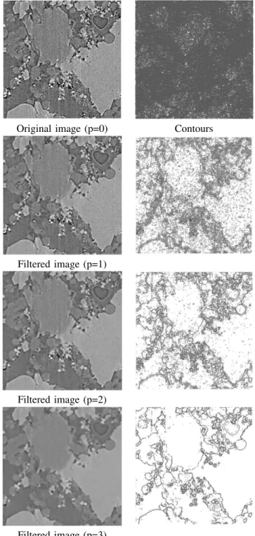
In Figure 5, we present the segmentation process on the images given by the filtering operation intermediate steps. The edge detector has been “set” to c = 0.75. One can see that the original image segmentation is quite poor: a lot of small contours that are generated by the noise appear.
Figure 6, shows the segmentation sensitivity process with respect to the edge detector and parameter c. It has been performed on the filtered image (n = 7, p = 3). If c is small we find contours that are quite constrasted : this gives the global structure of the material. A larger c provide the details via the less contrasted contours. We give the contours that are obtained with a standard Canny’s edge detector as well.
VI. CONCLUSION
We conclude that the mixture of different techniques gives an interesting segmentation of the images we consider. In-deed, the filtering step allows to get rid of the noise that would provide articial contours otherwise. With a suitable choice of a contour detector function (that we tune via the
c parameter) we have a hierarchical segmentation (from the very contrasted contours to the less ones) which can be adpated to the “textured areas” that appear when the stone is completely pulverulent. However, we try to improve the method : the filtering step can be performed with variational techniques (namely the Rudin-Osher-Fatemi model [27]) and the segmentation process is now investigated with a watershed approach.
Original image (p=0) Contours
Filtered image (p=1)
Filtered image (p=2)
Filtered image (p=3)
Fig. 5. Segmentation of filtered images with respect to p and c = 0.75.
REFERENCES
[1] C. R. Appoloni, C. P. Fernandes and C. R. O. Rodrigues, X-ray tomography study of a sandstone reservoir rock, Nuclear instruments and methods in physics research A, 580:629632, 2007.
[2] J.F. Aujol, Traitement d’images par approches variationnelles et ´equations aux d´eriv´ees partielles, Semestre d’enseignement UNESCO sur le traitement des images num´eriques, Tunis, ENIT, Avril 2005. [3] J. Baruchel, J.-Y. Buffiere, P. Cloetens, M. Di Michiel, E. Ferrie, W.
Ludwig, E. Maire and L. Salvo, Advances in synchrotron radiation microtomography, Scripta Materialia, 55:4146, 2006.
[4] J. Baruchel, J.-Y. Buffiere, E. Maire, P. Merle and G. Peix, X-Ray Tomography in Material Science, Hermes, 2000.
[5] M. Bergounioux, and L. Guillot, Existence and uniqueness results for the Gradient Vector Flow and geodesic active contours mixed model, submitted, 2007.
Filtered image Canny’s algorithm
c = 0.25 c = 0.5
c = 0.75 c = 1
Fig. 6. Segmentation with p = 3 and different values of c. Comparison with Canny’s edge detector.
[6] M. Betson, J. Barker, P. Barnes and T. Atkinson, Use of synchrotron tomographic techniques in the assessment of diffusion parameters for solute transport in groundwater flow, Transport in Porous Media, 60:217223, 2005.
[7] A. Carminati, A. Kaestner, O. Ippisch, A. Koliji, P. Lehmann, R. Hassanein, P. Vontobel, E. Lehmann, L. Laloui, L. Vulliet and H. Fluhler. Water flow between soil aggregates. Transport in Porous Media, 68:219236, 2006.
[8] D. Cammuffo, Physical weathering of stones, Sci. Total Environ. 167:1-14, 1995.
[9] V. Caselles, R. Kimmel and G. Sapiro, Geodesic Active Contours, International Journal of Computer Vision, Vol. 22, 1, 1997, pp. 61-79. [10] R. Deriche and O. Faugeras, Les EDP en Traitement des Images et
Vision par Ordinateur, Traitement du Signal, 13, 1996.
[11] D. Dessandier. ´Etude du milieu poreux et des propri´et´es de transfert des fluides du tuffeau blanc de Touraine. Application `a la durabilit´e des pierres en œuvre. PhD thesis, University of Tours, France, 1995. [12] S.T. Erdogan, P.N. Quiroga, D.W. Fowler, H.A. Saleh, R.A. Livingston,
E.J. Garboczi, P.M. Ketcham, J.G. Hagedorn and S.G. Satterfield. Three-dimensiona l shape analysis of coarse aggregates: New techniques for and preliminary results on several different coarse aggregates and reference rocks. Cement and Concrete Research, 36:16191627, 2006. [13] E. Galan, M.I. Carretero and E. Mayoral. A methodology for locating the
original quarries used for constructing historical buildings: application to malaga cathedral, spain. Engineering Geology, 54:287298, 1999. [14] P.L. Gaspar and J. de Brito, Quantifying environmental
ef-fects on cement-rendered facades: A comparison between dif-ferent degradation indicators, Building and Environment (2007), doi:10.1016/j.buildenv.2007.10.022
[15] L. Guillot, The Gradient Vector Flow and geodesic active contours mixed model applied to Tuffeau segmentation , preprint, 2008 [16] A. C. Jones, B. Milthorpe, H. Averdunk, A. Limaye, T. J. Senden,
A. Sakellariou, A. P. Sheppard, R. M. Sok, M. A. Knackstedt, A. Brandwood, D. Rohner and D. W. Hutmacher. Analysis of 3D bone ingrowth into polymer scaffolds via micro-computed tomography imag-ing. Biomaterials, 25:49474954, 2004.
[17] A. C. Kak and M. Slaney. Principles of Computerized Tomographic Imaging. Society for Industrial and Applied Mathematics, 2001. [18] S. Kichenassamy, A. Kumar, P. Olver, A. Tannenbaum and A. Yezzi,
Gradient Flows and Geometric Active Contour Models, Proc. IEEE Int. Conf. Computer Vision, vol.1, pp. 67-73, 2001.
[19] E. Le Trong, O. Rozenbaum, J.L. Rouet and A. Bruand, A methodology to segment X-ray tomographic images of multiphase porous media: application to building stones. Submitted to Image Analysis and Stere-ology, HAL-00260435
[20] G. Matheron. Random sets and integral geometry. Wiley, New York, 1975.
[21] S. Osher and N. Paragios, Geometric Level Set Sethods in Imaging, Vision, ad Graphics , Springer, 2003.
[22] S. Osher and Sethian Fronts propagating with curvature-dependent velocity : algorithms based on the Hamilton-Jacobi formulation, Journal of Computational Physics, 79, pp. 12-49, 1988.
[23] N. Paragios, O. Mellina-Gottardo and V. Ralmesh, Gradient Vector Flow Fast Geodesic Active Contours, Proc. IEEE Int. Conf. Computer Vision, vol.1, pp. 67-73, 2001.
[24] S. Rolland du Roscoat, J.-F. Bloch and X. Thibault. Synchrotron radiation microtomography applied to investigation of paper. Journal of Physics D: Applied Physics, 38(10):7884, 2005.
[25] O. Rozenbaum, E. Le Trong, J. L. Rouet and A. Bruand. 2d-image analysis: A complementary tool for characterizing quarry and weathered building limestones. Journal of Cultural Heritage, 8:151159, 2007. [26] L. Salvo, P. Cloetens, E. Maire, S. Zabler, J. J. Blandin, J.-Y. Buffiere, W.
Ludwig, E. Boller, D. Bellet and C. Josserond. X-ray microtomography an attractive characterisation technique in materials science. Nuclear Instruments and Methods in Physics Research Section B: Beam Inter-actions with Materials and Atoms, 200:273286, 2003.
[27] L. Rudin, S. Osher and E. Fatemi, Nonlinear total variation based noise removal algorithms, Physica D, 60, 1992, pp. 259-268.
[28] J. Serra, Image analysis and mathematical morphology. AcademicPress, London, 1982.
[29] J. A. Sethian, Level Set Methods, Cambridge University Press, 1996. [30] A. P. Sheppard, R. M. Sok and H. Averdunk. Techniques for image
en-hancement and segmentation of tomographic images of porous materials. Physica A, 339:145151, 2004.
[31] D. Terzopoulos, A. Witkin and M. Kass, Snakes : Active contour models, International Journal of Computer Vision, Vol. 1, 1988, pp. 321-331. [32] C. Xu and J.L. Prince, Gradient Vector Flow : A new external force for
snakes, IEEE Proc. Conf. on Comp. Vis. Patt. Recog. (CVPR’97), 1997, pp. 66-71.
[33] C. Xu and J.L. Prince, Snakes, Shapes, and Gradient Vector Flow, IEEE Transactions on image processing, Vol.7, 3, pp. 359-369, March 1998. [34] C. Xu, A. Yezzi and J.L. Prince, On the relationship between parametric and geometric active contours, In Proc. of 34th Asilomar Conference on Signals, Systems, and Computers, pp. 483-489, October 2000.
Laurence Guillot PhD. student in mathematics at the University of Orleans. Her research interests are in the areas of image processing, segmentation by geodesic active contours and gradient vector flow.
Emmanuel Le Trong Doctor in mechanics (2003) is currently postdoctoral fellow at the Institut des Sciences de la Terre dOrlans . His main research interest is the relation between the microstructure of a porous medium and its macroscopic transport properties.
Olivier Rozenbaum Doctor in physical sciences (1999), Assistant Professor at the University of Orlans and member of the Institut des Sciences de la Terre dOrlans . Since 2001, his works have been devoted to the study of the weathering of building stones. His research concerns (i) the characterization of porous media, notably by microtomography X and analysis of the resulting 3D images and (ii) the water transfer simulation at the pore scale.
Ma¨ıtine Bergounioux Full professor in mathematics at Orlans University. Her research fields are mathematical modelling, partial derivative equations, optimal control and optimization, signal and image processing.
Jean-Louis Rouet Doctor in physical sciences (1990), Full Professor at the University of Orlans. His works have been devoted to modelisation and simulation of long range interacting systems and in the social science area. More recently he joins the Institut des Sciences de la Terre dOrlans and works on water transfer simulation at building stones pore scale .