Call-by-Value Lambda-calculus and LJQ

HAL Id: hal-00150284

https://hal.archives-ouvertes.fr/hal-00150284

Preprint submitted on 30 May 2007

HAL is a multi-disciplinary open access

archive for the deposit and dissemination of

sci-entific research documents, whether they are

pub-lished or not. The documents may come from

teaching and research institutions in France or

abroad, or from public or private research centers.

L’archive ouverte pluridisciplinaire HAL, est

destinée au dépôt et à la diffusion de documents

scientifiques de niveau recherche, publiés ou non,

émanant des établissements d’enseignement et de

recherche français ou étrangers, des laboratoires

publics ou privés.

Call-by-Value Lambda-calculus and LJQ

Roy Dyckhoff, Stéphane Lengrand

To cite this version:

Call-by-Value λ-calculus and LJQ

Roy Dyckhoff and Stéphane Lengrand

School of Computer Science,

University of St Andrews,

St Andrews, Fife,

KY16 9SX, Scotland.

{rd,sl}@dcs.st-and.ac.uk

19th April 2007

LJQis a focused sequent calculus for intuitionistic logic, with a simple re-striction on the first premiss of the usual left introduction rule for implication. In a previous paper we discussed its history (going back to about 1950, or be-yond) and presented its basic theory and some applications; here we discuss in detail its relation to call-by-value reduction in lambda calculus, establishing a connection between LJQ and the CBV calculus λCof Moggi. In particular,

we present an equational correspondence between these two calculi forming a bijection between the two sets of normal terms, and allowing reductions in each to be simulated by reductions in the other.

Keywords: lambda calculus, call-by-value, sequent calculus, continuation-passing, semantics

1

Introduction

Proof systems for intuitionistic logic are well-known to be related to compu-tation. For example, a system of uniform proofs for Horn logic is a coherent explanation of proof search in pure Prolog, as argued by (e.g.) [17]; likewise, natural deduction corresponds under the Curry-Howard correspondence to the ordinary typed λ-calculus, with beta-reduction, i.e. to the classic model of computation for typed functional programs.

Similarly, the sequent calculus can also be related to computation via the process of cut-elimination. In particular, two intuitionistic sequent calculi LJT and LJQ, presented in Herbelin’s thesis [10] and based on earlier work [14], [2] by Joinet et al, feature cut-elimination systems in connection with call-by-name (CBN) and call-by-value (CBV) semantics, respectively.

Such semantics apply to functional programming [20] and concern the choice of evaluating an argument after or (resp.) before being passed to a function.

The λ-calculus is so pure a model for functional programs that any compu-tation is, in a sense defined in [20], call-by-name. This relates to the sequent calculus LJT whose notion of focus [1] establishes a close connection with nat-ural deduction, of which the λ-calculus is a proof-term language. The cut-free proofs of LJT are in 1-1 correspondence with the normal natural deductions; LJThas a well-developed theory of proof-reduction with strong normalisation [11, 5, 3] that relates to the normalisation of the simply-typed λ-calculus. Note that LJT itself can be given with proof-terms, which help formalising such con-nections directly with call-by-name (i.e. unrestricted) λ-calculus; these terms are meaningful even in an untyped setting.

Likewise, LJQ (as presented in [4]) is a focused sequent calculus, captur-ing a simple restriction on proofs significant for structural proof theory and automated reasoning. In [10], LJQ is related to Lorenzen dialogues, but the suggested connection with call-by-value semantics has never, as far as we are aware, been formalised as a relation between cut-elimination in LJQ and nor-malisation in a call-by-value (λ-)calculus.

Addressing this issue raises the questions of what call-by-value λ-calculus is, and what cut-elimination process specific to LJQ is to be used. These ques-tions have very satisfying answers for CBN and LJT(c.f. [11, 5, 3]); extending (for implicational logic) the brief discussion in [4], the present paper

• formalises, by means of a proof-term calculus, a cut-elimination system specific to LJQ and its particular notion of focus,

• optimises a CBV λ-calculus due to Moggi [18], so that it satisfies finer semantical properties and thus better connects to LJQ,

• proves the confluence of the obtained calculi and relates them by using notions of abstract rewriting such as equational equivalences.

The logical inspiration for this investigation is strong, but once proof-terms are considered, all results in this paper hold even in an untyped framework.

Call-by-valueλ-calculus

Recall that CBV λ-calculus partially (and only partially) captures the com-mon convention, in implementation of functional languages, that arguments are evaluated before being passed to functions. The fundamental ideas are explored by Plotkin in [20], where a calculus λV is introduced; its terms are

exactly those of λ-calculus and its reduction rule βV is merely β-reduction

restricted to the case where the argument is a value V , i.e. a variable or an abstraction.

βV (λx.M ) V −→ M {x = V }

Clearly, in the fragment λEvalArg of λ-calculus where all arguments are

values, βV = β. Hence, applying CBN- (general β) or CBV- (βV) reduction

is the same, a property that is called strategy indifference; therefore, in the context of λEvalArg, we will not distinguish βV from β.

Using the notion of continuation, of which a history can be found in [22], the (CBN) λ-calculus can be encoded [20] into λEvalArg with a

continuation-passing-style (CPS) translation in a way such that two terms are β-equivalent if and only if their encodings are β-equivalent.

Similarly, for the CBV calculus λV, two CPS-translations into λEvalArgcan

be defined: Reynolds’ [21, 23] and Fischer’s [7, 8]. Both are sound, in that in each case any two βV-equivalent λ-terms are mapped to two β-equivalent

terms, but they are both incomplete in that the β-equivalence in λEvalArg is

bigger than needed (see e.g. [20]).

This problem is solved by Moggi’s calculus λC[18]; this extends λV with

a let _ = _ in _ constructor and new reduction rules, such as:

letV letx = V in M −→ M {x = V }

In particular, with the use of this new constructor, an application cannot be a normal form if one of its components is not a value. Both the aforementioned CPS-translations on λV can be extended to λC, in a way such that they are

both sound and complete.

Thus, equivalence in the extended CBV λ-calculus λC of Moggi can be

modelled by equivalence in λEvalArg; but (as we show below) this modelling

does not extend to modelling of reductions. Our more refined analysis, pre-sented in this paper, of the CBV λ-calculus λCconsiders how reductions, rather

than equivalence, are modelled by CPS-translations. Here the crucial concept is that of a reflection, i.e. a reduction-preserving encoding that makes one calculus isomorphic to a sub-calculus of another. Already in [25], a refined

Reynolds translation is proved to form a reflection in λCof its target calculus

λR CPS.

However, [25] states that a particular refined Fischer translation cannot be a reflection. We show here that a different (and more natural) refined version of the Fischer translation that does form a reflection of its target calculus λF

CPS

in (a minor variation of) λC.

We leave the discussion about the different refinements for section 3.1. The minor variation of λCconsists of the replacement of rule βVwith the following:

B (λx.M ) N −→ let x = N in M

This change is justified for three reasons:

• It does not change the equational theory of λC.

• Splitting βVinto B followed by letVseems more atomic and natural, with

only one rule controlling whether a particular sub-term is a value or not. • This variation makes our refined Fischer translation a reflection in λCof

its target calculus.

From the reflection result we can also prove that our version of λC is

confluent (Theorem 1), using the confluence of λF CPS.

In summary, then, we are able to show that a minor variation of Moggi’s calculus λCis a natural candidate as the canonical CBV λ-calculus, admitting

two CPS-translations each of which not merely models equivalences but also models reductions. We turn now to using this as a basis for considering the properties of LJQ -as a CBV sequent calculus (analogous to the use of CBN λ-calculus in relation to the properties of LJT as a CBN sequent calculus, viz. strong normalisation, confluence and simulation of β-reduction).

LJQ

The history of LJQ goes back to Vorob’ev [26] (detailing ideas published in 1952), who showed (his Theorem 3) that, in a minor variant of Gentzen’s calculus LJ for intuitionistic logic, one may, without losing completeness, re-strict instances of the left rule L⊃ for implication to those in which, if the antecedent A of the principal formula A⊃B is atomic, then the first premiss is an axiom. Much later, Hudelmaier [12] showed that one could further restrict this rule to those instances where the first premiss was either an axiom or the conclusion of a right rule; the result was proved in his thesis [12] and described in [13] as folklore. The same result is mentioned by Herbelin in [10] as the completeness of a certain calculus LJQ, described simply as LJ with the last-mentioned restriction.

Following our approach in [4], we formalise such a restriction on LJ as a focussed calculus with two forms of sequent, ordinary sequents and focussed sequents. We also use proof-terms, so that LJQ becomes the typing system of a calculus called λQwith two syntactic categories, that of (ordinary) terms

and that of values. These are respectively typed by ordinary sequents and focussed sequents.

Letting Γ range over environments (i.e. finite functions from variables to formulae), we have the ordinary sequent Γ ⇒ M : A to express the deducibility (as witnessed by the term M ) of the formula A from the assumptions Γ, and the focussed sequent Γ → M : A to impose the restriction that the last step in the deduction is by an axiom or a right rule (i.e. with the succedent formula principal).

The rules of the calculus are then as presented below, in Sect. 4. For ex-ample, the rule L⊃ has, as conclusion and second premiss, ordinary sequents, but as first premiss a focussed sequent, capturing the restriction on proofs discussed by Hudelmaier (given that the focussed sequents are exactly the axioms or the conclusions of right introduction rules).

λQ can be considered independently from typing, while its notion of

re-duction (not necessarily representing proof transformations) still expresses the call-by-value operational semantics of the calculus. This is revealed by continuation-passing style translations [22] and relates to Moggi’s call-by-value calculus λC[18], modified as outlined above.

The connection between λQ and λCcan be summarised as follows: There

are encodings from λQto λCand from λCto λQsuch that

• they form a bijection between cut-free terms (a.k.a. normal forms) of λQ

and normal forms of λC,

• they form an equational correspondence between λQand λC,

• the reductions in λQare simulated by those of λC,

• the reductions in λCare simulated by those of λQ.

Thus, LJQ can be considered as a sequent calculus version of a canonical CBVλ-calculus (our modified Moggi calculus λC) in the same way that LJT

has been shown [3] to be a sequent calculus version of the CBN λ-calculus.

Structure of the paper

Section 2 is a preliminary section that presents the main tools that are used to relate λQ to λC. Section 3.1 presents Plotkin’s CBV λV-calculus [20] and

the CPS-translations from λV. Section 3.2 identifies the target calculi λRCPS

and λF

CPS, and proves the confluence of λFCPS. Section 3.3 presents Moggi’s

calculus λC [18] extending λV, introducing the aforementioned variant, and

in section 3.4 we prove that the Fischer translation forms a reflection in (our slightly modified version of) λCof λFCPS. In section 4 we present (at last) the

calculus λQ, including its reduction system. Section 5 investigates the CBV

semantics of λQ, via an adaptation of the Fischer CPS-translation. Section 6

combines the results of the previous sections to express the connection between λQand λC. Section 7 concludes with directions for further work.

2

Preliminary notions

In this section we recall some concepts (mainly from [16]) about reduction relations, especially notions used to relate one calculus to another.

Definition 1 (Simulation) Let R be a total function from a set A to a set B, respectively equipped with the reduction relations →Aand →B.

→B weakly simulates →A through R if for all M, M′ ∈ A, M →A M′

implies R(M ) →∗

BR(M′).

The notion of strong simulation is obtained by replacing R(M ) →∗ B R(M

′₎

by R(M ) →+ B R(M

′_{) in the above definition, but in this paper we only deal}

with weak simulation and thus abbreviate it as “simulation”.

We now define some more elaborate notions based on simulation, such as equational correspondence [24], Galois connection and reflection [16]. A useful account of these notions, with intuitive explanations, can be found for instance in [25]. In the following definition and in the rest of the paper, we write f · g for the functional composition that maps an element M to g(f (M )).

Definition 2 (Galois connection, reflection & related notions) Let A and B be sets respectively equipped with the reduction relations →A

and →B. Consider two mappings f : A −→ B and g : B −→ A.

• f and g form an equational correspondence between A and B if the following conditions hold:

– If M →AN then f (M ) ↔∗Af (N )

– f · g ⊆↔A

– g · f ⊆↔B

• f and g form a Galois connection from A to B if the following conditions hold: – →B simulates →A through f – →A simulates →B through g – f · g ⊆→∗ A – g · f ⊆←∗ B

• fand g form a pre-Galois connection from A to B if in the four conditions above we remove the last one.

• f and g form a reflection in A of B if the following conditions hold: – →B simulates →A through f

– →A simulates →B through g

– f · g ⊆→∗ A

– g · f = IdB

Note that saying that f and g form an equational correspondence be-tween A and B only means that f and g extend to a bijection bebe-tween ↔A

-equivalence classes of A and ↔B-equivalence classes of B. If f and g form an

equational correspondence, so do g and f ; it is a symmetric relation, unlike (pre-)Galois connections and reflections.

A Galois connection provides both an equational correspondence and a pre-Galois connection. A reflection provides a Galois connection. Also note that if f and g form a reflection then g and f form a pre-Galois connection.

The notions of equational correspondence, pre-Galois connection, Galois connection, and reflection are transitive notions, in that, for instance, if f and g form a reflection in A of B and f′ _{and g}′ _{form a reflection in B of C}

then f · f′ and g · g′ form a reflection in A of C (and similarly for equational correspondences, pre-Galois connection and Galois connections).

These notions based on simulation can then be used to infer, from the confluence of one calculus, the confluence of another calculus. This technique is also known as the Interpretation Method [9].

Theorem 1 (Confluence by simulation) If f and g form a pre-Galois connection from A to B and →B is confluent, then →A is confluent.

Proof: The proof is graphically represented in Fig. 1. ✷

3

Call-by-value λ-calculus

In this section we present some new developments in the theory of CBV λ-calculus.

3.1

λ

& CPS-translations

We present the λV-calculus of [20]:

Definition 3 (λV) The syntax of λV is the same as that of λ-calculus,

al-though it is elegant to present it by letting values form a syntactic category of their own:

V, W, . . . ::= x | λx.M M, N, . . . ::= V | M N V, W, . . .stand for values, i.e. variables or abstractions.

∗ AGGG_G## G G G G G ∗ A {{wwww wwww f ®¶ ∗ A »» f ®¶ f ®¶ ∗ A §§ ∗ BGGG_G## G G G G G ∗ B {{wwww wwww ∗ BGGG_G## G G G G G g ®¶ ∗ B {{wwww wwww g ®¶ g ®¶ ∗ A ## G G G G G G G G G ∗ A {{wwww wwww w

Figure 1: Confluence by simulation

We obtain the reduction rules of λVby restricting β-reduction to the cases

where the argument is a value and restricting η-reduction to the cases where the function is a value:

βV (λx.M ) V −→ M {x = V }

ηV λx.V x −→ V if x 6∈ FV(V )

In presence of βV, the following rule has the same effect as ηV:

η′V λx.y x −→ y if x 6= y

Definition 4 (λEvalArg) λEvalArgis the fragment of λ-calculus where all

argu-ments are values, hence given by the following syntax:

V, W, . . . ::= x | λx.M M, N, . . . ::= V | M V

Remark 2 (Strategy indifference) In the λEvalArg fragment, βV = β, so

applying CBN- (general β) or CBV- (βV) reduction is the same.

Note that the situation is different for η-conversion in λEvalArg, since ηV6= η.

The fragment λEvalArgis stable under βV/β-reduction and under ηV-reduction,

but not under η-reduction.

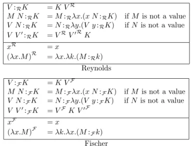
We can encode λV into λEvalArg by using the notion of continuation and

defining Continuation Passing Style translations (CPS-translations). There are in fact two variants of the CBV CPS-translation: Reynolds’ [21, 23] and Fischer’s [7, 8], presented in Fig. 2.

Note that the two translations only differ in the order of arguments in x y k/ x k y and λx.λk.R(M ) k / λk.λx.F(M ) k.

As mentioned in the introduction, both translations map βV-equivalent

terms to β/βV-equivalent terms (soundness), but the converse fails

(incom-pleteness) (see e.g. [20]).

A more refined analysis is given by looking at the reduction rather than just equivalence. Note that the two translations above introduce many fresh variables, but bind them, often leading to new redexes and potential redexes not corresponding to redexes in the original terms. Some of these get in the way of simulating β-reduction of the original terms. However, they can be identified as administrative, so that the translations above can be refined by

R(V ) = λk.k RV(V ) R(M N ) = λk.R(M ) (λx.R(N ) (λy.x y k)) RV(x) = x RV(λx.M ) = λx.λk.R(M ) k Reynolds’ translation F(V ) = λk.k FV(V ) F(M N ) = λk.F(M ) (λx.F(N ) (λy.x k y)) FV(x) = x FV(λx.M ) = λk.λx.F(M ) k Fischer’s translation

Figure 2: CBV CPS-translations, from λVto λEvalArg

reducing these redexes. The precise definition of which redexes are adminis-trative is crucial, since this choice might or might not make the refined Fischer translation a Galois connection or a reflection (Definition 2), as we shall see in section 3.4. In Fig. 3 we give the refinement for a particular choice of ad-ministrative redexes. In this figure, K ranges over λ-terms. We shall see that, for the inductive definition to work, it is sufficient to restrict the range of K to particular terms called continuations.

V :RK = K VR

M N :RK = M :Rλx.(x N :RK) if M is not a value

V N :RK = N :Rλy.(V y :RK) if N is not a value

V V′_: RK = VR V′RK xR _{= x} (λx.M )R = λx.λk.(M :Rk) Reynolds V :FK = K VF M N :FK = M :Fλx.(x N :FK) if M is not a value

V N :FK = N :Fλy.(V y :FK) if N is not a value

V V′_:

FK = VFK V′F

xF _{= x}

(λx.M )F = λk.λx.(M :Fk)

Fischer

Figure 3: Refined CBV CPS-translations, from λVto λEvalArg

We first prove that the refined translations are indeed obtained by reduc-tion of the original ones.

Lemma 3

1. RV(V ) −→∗_β VR and R(M) K −→∗_β M :RK

2. FV(V ) −→∗_β VF and F(M) K −→∗_β M :FK

Proof: For each point the two statements are proved by mutual induction on V and M . The interesting case is for M = M1M2, which we present with

the Fischer translation (the case of Reynolds is very similar): F(M1M2) K =

F(M1) (λx.F(M2) (λy.x K y)) −→β M1:F(λx.N :F(λy.x K y))by induction

hypothesis.

• If neither M1 nor M2 are values, this is also

• If M1 is a value and M2 is not, this is also

(λx.M2:F(λy.x K y)) M1F −→β M2:F(λy.M1FK y) = M1M2:FK.

• If M1 is not a value but M2 is, this is also

M1:F(λx.(λy.x K y) M2F) −→β M1:F(λx.x K M2F) = M1M2:FK.

• If both M1 and M2are values, this is also

(λx.(λy.x K y) M2F) M1F−→∗_β M1F K M2F= M1M2:FK.

✷

Remark 4 Note that K is a sub-term of M :RK and M :FK with exactly

one occurrence1_{, so for instance if x ∈ FV(K) \ FV(M ) then x has exactly one}

free occurrence in M :RKand M :FK. Hence, the variables introduced by the

translations and denoted by k, which we call the continuation variables, are such that the set of those that are free in the scope of a binder λk. is exactly {k}, with exactly one occurrence (only one of them can be free at a time).

In other words, in a term (which is a α-equivalence class of syntactic terms, i.e. a set) there is always a representative that always uses the same variable k. Note that K does not need to range over all λ-terms for the definition of the refined translations to make sense, but only over constructs of the form k or λx.M , with x 6= k.

In that case, note that if we call continuation redex any β-redex binding a continuation variable (i.e. any redex of the form (λk.M ) N ), then the refined Reynolds translation considers all continuation redexes to be administrative and has thus reduced all of them, while the refined Fischer translation leaves a continuation redex in the construct (λx.M ) V :FK = (λk.λx.M :Fk) K VF,

which is thus not administrative.

This choice is different from that of [25] which, as for the Reynolds transla-tion, considers all continuation redexes to be administrative. With that choice the authors establish negative results about the refined Fischer translation as we shall discuss in section 3.4.

We can now identify the target calculi of the refined translations, i.e. the fragments of λ-calculus reached by them, and look at their associated notions of reduction.

3.2

The CPS calculi λ

CPS

& λ

From the refined Reynolds and Fischer translations we get the target frag-ments of λ-calculus described in Fig. 4.

• M, N, . . .denote (CPS-)programs, • V, W, . . .denote (CPS-)values, • K, K′_{, . . .denote continuations.} M, N ::= K V | V W K V, W ::= x | λx.λk.M with k ∈ FV(M ) K ::= k | λx.M M, N ::= K V | V K W V, W ::= x | λk.λx.M with k ∈ FV(λx.M ) K ::= k | λx.M Reynolds: λR CPS Fischer: λFCPS

Figure 4: Target calculi

Note that values have no free occurrence of continuation variables while programs and continuations have exactly one. Also note that x ranges over an infinite set of variables, while for every term it is always possible to find a rep-resentative (i.e. a syntactic term) that uses a paricular continuation variable k. In fact we could have a constructor with arity 0 to represent this variable

1_{In some sense the construction _ :}

and a constructor with arity 1 for λk._, but treating k as a variable allows the use of the implicit substitution of k.

The fragments are stable under the reductions in Fig. 5 and are sufficient to simulate βVand ηVthrough the CPS-translations, as we shall see in section 3.4.

We write λR

CPSβ (resp. λFCPSβ) for system βV1, βV2and λRCPSβη (resp. λFCPSβη)

for system βV1, βV2, ηV1, ηV2in λRCPS (resp. λ F CPS). βV1 (λx.M ) V −→ M {x = V } βV2 (λx.λk.M ) V K −→ M {x = V }{k = K} ηV1 λx.λk.V x k −→ V if x 6∈ FV(V ) ηV2 λx.K x −→ K if x 6∈ FV(K) Reynolds βV1 (λx.M ) V −→ M {x = V } βV2 (λk.λx.M ) K V −→ (λx.M {k = K}) V ηV1 λk.λx.V k x −→ V if x 6∈ FV(V ) ηV2 λx.K x −→ K if x 6∈ FV(K) Fischer

Figure 5: Reduction rules for λR

CPS & λFCPS

Note the difference between the case of Reynolds and that of Fischer in the rule βV2. Reynolds-βV2 must perform two βV-reduction steps, since

(λk.M {x = V }) K is not a program of the fragment. Fischer-βV2performs

only one βV-reduction step, (λx.M {k = K}) V being a valid program. It could

obviously reduce further to M {k = K}{x = V } as for the case of Reynolds, but leaving this second step as a βV1-reduction has nice properties: this split

of reduction into two atomic βV-steps makes the refined Fischer translation

(as defined here) a reflection.

A good account of the refined Reynolds translation as a reflection can be found in [25], so here we study similar properties for the refined Fischer translation, building on earlier work [24] that established results of equational correspondence. Moreover, Fischer’s approach helps establish connections be-tween CBV-λ-calculus and LJQ from section 4.

We now establish the confluence of λF

CPS. The confluence of λFCPSβ is

straightforward, since every case of β-reduction in λF

CPS is covered by either

βV1 or βV2, so it is a particular case of the confluence of β-reduction in

λ-calculus. For λF

CPSβη we use the confluence of β, η-reduction in λ-calculus, but

un-fortunately the language of λF

CPS is not stable under β, η. Fig. 6 shows its

closure λ+

CPS under β, η. Such a closure is used for instance in [24].

M, N ::= K V V, W ::= x | λk.K K ::= k | λx.M | V K Figure 6: Grammar of λ+

CPS

First, note that we no longer have β = βV. Second, this grammar is indeed

stable under β, η; all the cases are:

(λx.M ) V −→β M {x = V }

(λk.K) K′ _−→

β K{k = K′}

λk.V k −→η V

λx.K x −→η K if x 6∈ FV(K)

We can then take β, η as the reductions of λ+

CPS, and derive from the

confluence of λ-calculus that β and η are confluent in λ+ CPS.

Note that λ+

CPSis the smallest language that includes that of λ F

CPSand that

is stable under β, η: Fig. 7 defines a mapping ⇑ from λ+

CPSonto λ F

⇑ M −→η M. Our convention for parentheses assumes that ⇑ applies to the

smallest expression on its right-hand side. ⇑ (k V ) = k ⇑ V ⇑ ((λx.M ) V ) = (λx. ⇑ M ) ⇑ V ⇑ (W K V ) =⇑ W ⇑ K ⇑ V ⇑ x = x ⇑ λk.k = λk.λx.k x ⇑ λk.λx.M = λk.λx. ⇑ M ⇑ λk.V K = λk.λx. ⇑ V ⇑ K x ⇑ k = k ⇑ λx.M = λx. ⇑ M ⇑ (V K) = λx. ⇑ V ⇑ K x Figure 7: Projection of λ+ CPS onto λFCPS

Remark 5 Note that ⇑ M −→η M, ⇑ V −→η V, ⇑ K −→η K and if M ,

V, K are in λF

CPS then ⇑ M = M , ⇑ V = V , ⇑ K = K.

We can now prove the following:

Theorem 6 (⇑ is a Galois connection) The identity Id_λF

CPS and the

map-ping ⇑ form a Galois connection from λF

CPS, equipped with λ F

CPSβη, to λ + CPS,

equipped with βV (and also with only λFCPSβ and β).

Proof: Given Remark 5, it suffices to check the simulations: • For the simulation of η by λF

CPSβη through ⇑, we check all cases:

⇑ λk.λx.k x = λk.λx.k x = ⇑ λk.k

⇑ λk.λx.(λy.M ) x = λk.λx.(λy. ⇑ M ) x −→ηV2 λk.λy. ⇑ M = ⇑ λk.λy.M

⇑ λk.λx.V K x = λk.λx. ⇑ V ⇑ K x = ⇑ λk.V K ⇑ λk.V k = λk.λx. ⇑ V k x −→ηV1 ⇑ V

⇑ λx.k x = λx.k x −→ηV2 k = ⇑ k

⇑ λx.(λy.M ) x = λx.(λy. ⇑ M ) x −→ηV2 λy. ⇑ M = ⇑ λy.M

⇑ λx.V K x = λx. ⇑ V ⇑ K x = ⇑ V K

For the simulation of β by λF

CPSβηthrough ⇑, we must first check:

⇑ M {x =⇑ V } =⇑ M {x = V } ⇑ M {k =⇑ K} −→∗ βV1⇑ M {k = K} ⇑ W {x =⇑ V } =⇑ W {x = V } ⇑ W {k =⇑ K} −→∗βV1⇑ W {k = K} ⇑ K′_{{x =⇑ V } =⇑ K}′_{{x = V } ⇑ K}′_{{k =⇑ K} −→}∗ βV1⇑ K ′_{{k = K}}

The left-hand side equalities and the right-hand side equalities are re-spectively proved by mutual induction on terms, with the following in-teresting case: ⇑ (k V ){k =⇑ K} = ⇑ K ⇑ V {k =⇑ K} by i.h. −→∗ βV1 ⇑ K ⇑ V {k = K} −→∗βV1 ⇑ (K V {k = K}) = ⇑ (k V ){k = K}

The penultimate step is justified by the fact that ⇑ K ⇑ V −→∗ βV1 ⇑

(K V )(it is an equality for K = k or K = λx.M and one βV1-reduction

step for K = W K′_).

We now checks all cases for β-reduction. The last step for the simulation of the β-reduction of a value is an equality if K′_{{k = K} = k}′ _{and one}

⇑ ((λx.M ) V ) = (λx. ⇑ M ) ⇑ V −→βV1 ⇑ M {x =⇑ V } = ⇑ M {x = V } ⇑ ((λk.k) K V ) = (λk.λx.k x) ⇑ K ⇑ V −→∗ βV2,βV1 ⇑ K ⇑ V −→∗ βV1 ⇑ (K V ) ⇑ ((λk.λx.M ) K V ) = (λk.λx. ⇑ M ) ⇑ K ⇑ V −→βV2 (λx. ⇑ M ){k =⇑ K} ⇑ V −→∗ βV1 ⇑ ((λx.M {k = K}) V ) ⇑ ((λk.W K′_{) K V ) = (λk.λx. ⇑ W ⇑ K}′_{x) ⇑ K ⇑ V} −→∗βV2,βV1 ⇑ W ⇑ K ′ {k =⇑ K} ⇑ V −→∗ βV1 ⇑ (W (K ′_{{k = K}) V )} ⇑ λk′_.(λk.K′_{) K = λk}′_{.λx. ⇑ (λk.K}′_{) ⇑ K x} −→∗ βV2,βV1 λk ′_{.λx. ⇑ (K}′_{{k = K}) x as above} −→∗ βV1 ⇑ λk ′_.K′_{{k = K}} ⇑ ((λk.K′_{) K) = λx. ⇑ (λk.K}′_{) ⇑ K x} −→∗ βV2,βV1 λx. ⇑ (K ′_{{k = K}) x as above} −→ηV2 ⇑ K′{k = K}

• The fact that β, η simulate βV1, βV2, ηV1, ηV2through Id_λF

CPS is trivial,

since the latter are particular cases of the former.

✷

Corollary 7 (Confluence of λF

CPS) λFCPSβ and λFCPSβη are confluent.

Proof: The first system is confluent as it is the entire β-reduction relation in λFCPS, the second system is confluent by Theorem 6 and Theorem 1. ✷

3.3

Moggi’s λ

-calculus

Both the refined Reynolds translation and the refined Fischer translations suggest to extend λV with a construct let _ = _ in _ with the following

semantics:

(let x = M in N ) :RK = M :Rλx.(N :RK)

(let x = M in N ) :FK = M :Fλx.(N :FK)

and with the following rules:

M N −→ let x = M in (x N ) if M is not a value V N −→ let y = N in (V y) if N is not a value

Indeed, for both refined translations, a redex of these rules and its reduced form are mapped to the same term.

This extension is related to Moggi’s monadic λ-calculus [19], which sug-gests additional rules, thus forming the CBV-calculus λC [18]2 defined as

fol-lows:

Definition 5 (λC) The terms of λCare given by the following grammar:

V, W, . . . ::= x | λx.M

M, N, P, . . . ::= V | M N | let x = M in N

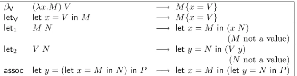
The reduction system of λCis given in Fig. 8.

Again, η-reduction can be added: ηlet letx = M in x −→ M

ηV λx.(V x) −→ V if x 6∈ F V (V )

βV (λx.M ) V −→ M {x = V } letV letx = V in M −→ M {x = V } let1 M N −→ let x = M in (x N ) (M not a value) let2 V N −→ let y = N in (V y) (N not a value) assoc lety = (let x = M in N ) in P −→ let x = M in (let y = N in P )

Figure 8: Rules of λC

And again, in presence of βV, rule ηVhas the same effect as the following

one:

ηV′ λx.(y x) −→ y if x 6= y

For various purposes described in the introduction, here we also consider a slight variation of λC, in which reduction is refined by replacing the reduction

rule βV with the following:

B (λx.M ) N −→ let x = N in M

This allows the split of the rule βVinto two steps: B followed by letV. Note

that in B we do not require N to be a value. Such a restriction will only apply when reducing let x = N in M by rule letV.

System λCβ is B, letV, let1, let2, assocand λCβη is λCβ, ηlet, ηV.

In [24] it is shown that, in effect, Fischer’s translation forms an equational correspondence between (Moggi’s original) λCand λFCPS. In [25], Sabry and

Wadler establish not only that Reynolds’ translation form an equational cor-respondence between (Moggi’s original) λCand λRCPS, but the refined Reynolds

translation actually forms a reflection.

3.4

The refined Fischer translation is a reflection

In [25], Sabry and Wadler also establish that for a particular definition of administrative redex (namely, every β-redex with a binder on the continua-tion variable k is administrative), the refined Fischer translacontinua-tion cannot be a reflection, and from λCto λFCPS it cannot even be a Galois connection.

Here we show that our (different) choice of administrative redex for the Fischer translation (given in Fig. 3) makes it a reflection of λF

CPSin our version

of λC, where the rule βVis decomposed into two steps as described above. This

will also bring λCcloser to LJQ.

Lemma 8 1. (M :FK){k = K′} = M :FK{k = K′} 2. (M :FK){x = VF} = M {x = V } :FK{x = VF} and WF{x = VF} = (W {x = V })F. 3. If K −→_λF CPSβ K ′ _{then M :} FK −→_λF CPSβ M :FK ′

(and similarly for −→λF CPSβη ).

Proof: Straightforward induction on M for the first and third points and on M and W for the second. ✷

Theorem 9 (Simulation of λCin λFCPS) The reduction relation −→λCβ

(resp. −→λCβη ) is simulated by −→λF

CPSβ (resp. −→λ F

CPSβη ) through the

refined Fischer translation.

Proof: By induction on the size of the term being reduced: We check all the root reduction cases, relying on Lemma 8:

((λx.M ) V ) :FK = (λk.λx.(M :Fk)) K VF

(Lemma 8.1) −→βV2 (λx.(M :FK)) VF

= (let x = V in M ) :FK

((λx.M ) N ) :FK = N :Fλy.(λk.λx.(M :Fk)) K y

(N not a value) (Lemma 8) −→∗

βV2,βV1N :Fλx.(M :FK) = (let x = N in M ) :FK (let x = V in M ) :FK = (λx.M :FK) VF −→βV1 (M :FK){x = VF} (Lemma 8.2) = (M {x = V }) :FK (M N ) :FK = M :Fλx.(x N :FK)

(M not a value) = (let x = M in x N ) :FK

(V N ) :FK = N :Fλx.(V x :FK)

(N not a value) = (let x = N in V x) :FK

(let y = (let x = M in N ) in P ) :FK = M :Fλx.(N :Fλy.(P :FK))

= (let x = M in (let y = N in P )) :FK

(let x = M in x) :FK = M :Fλx.K x

(Lemma 8.3) −→ηV2 M :FK

(λx.V x)F = λk.λx.VF k x −→ηV1 VF

The contextual closure is straightforward as well: only the side-condition “N is not a value” can become false by reduction of N . In that case if N −→λCβ

V we have N M :FK = N :Fλx.(x M :FK) by i.h. −→∗ λF CPSβ V :Fλx.(x M :FK) = (λx.(x M :FK)) VF −→βV1 V M :FK as well as: W N :FK = N :Fλx.(W x :FK) by i.h. −→∗ λF CPSβ V :Fλx.(W x :FK) = (λx.(W x :FK)) VF −→βV1 W V :FK

and also if M is not a value:

M N :FK = M :Fλx.(x N :FK)

by i.h. −→∗_λF

CPSβ M :Fλx.(x V :FK)

= M V :FK

and similarly with −→λF

CPSβη instead of −→λ F

CPSβ. ✷

Definition 6 (The Fischer reverse translation) We define a translation from λF

CPSto λC:

(k V )F back _{= V}F back

((λx.M ) V )F back = let x = VF back_inMF back

(W k V )F back = WF back_VF back

(W (λx.M ) V )F back = let x = WF back_VF back _inMF back

xF back _{= x}

Lemma 10

1. (W {x = V })F back_{= W}F back_{{x = V}F back_}and

(M {x = V })F back= MF back_{{x = V}F back_}.

2. let x = MF back_inNF back_−→∗

λCβ (M {k = λx.N })

F back_{(if k ∈ FV(M)).}

Proof: The first point is straightforward by induction on W , M . The second is proved by induction on M :

letx = (k V )F backinNF back

= letx = VF back _inNF back

= ((k V ){k = λx.N })F back letx = ((λy.P ) V )F back

inNF back

= letx = (let y = VF back inPF back) in NF back −→assoc lety = VF backin letx = PF back inNF back

by i.h. −→∗λCβ lety = V

F back

in(P {k = λx.N })F back = ((λy.P {k = λx.N }) V )F back

letx = (W k V )F backinNF back

= letx = WF back_VF back_inNF back

= (W (λx.N ) V )F back = ((W k V ){k = λx.N })F back

letx = (W (λy.P ) V )F backinNF back

= letx = (let y = WF back_VF back

in PF back_{) in N}F back

−→assoc lety = WF backVF back in letx = PF backinNF back

by i.h. −→∗λCβ lety = W

F back

VF back in(PF back{k = λx.N }) = (W (λy.PF back_{{k = λx.N }) V )}F back

= ((W (λy.P ) V ){k = λx.N })F back

✷

Theorem 11 (Simulation of λF

CPS in λC) The reduction relation −→λF CPSβ

(resp. −→λF

CPSβη ) is simulated by −→λCβ (resp. −→λCβη) through Fback.

Proof: By induction on the size of the term being reduced: We check all root reduction cases, relying on Lemma 10:

((λx.M ) V )F back = letx = VF back _inMF back

−→letV M

F back_{{x = V}F back_}

(Lemma 10) = (M {x = V })F back ((λk.λx.M ) k′_{V )}F back

= (λx.MF back_{) V}F back

−→B letx = VF back inMF back

= ((λx.M {k = k′_{}) V )}F back

((λk.λx.M ) (λy.N ) V )F back

= lety = (λx.MF back) VF backinNF back −→B lety = (let x = VF back inMF back) in NF back

= lety = ((λx.M ) V )F backinNF back (Lemma 10) −→λCβ (((λx.M ) V ){k = λy.N F back })F back (λk.λx.V k x)F back _{= λx.V}F back_x −→ηV V F back ((λx.K x) V )F back _−→ λCβ (K V ) F back _{by simulation of β} V1 (W (λx.k x) V )F back₌

letx = WF back_VF back

inx −→ηlet W F back VF back = (W k V )F back (W (λx.(λy.M ) x) V )F back

= letx = WF back_VF back

in lety = x in MF back

−→letV lety = W

F back

VF back inMF back = (W (λy.M ) V )F back

✷ Lemma 12 V −→∗ λCβ V F F back_{and M −→}∗ λCβ (M :Fk) F back .

Proof: By induction on the size of V , M . The cases for V (V = x and V = λx.M) are straightforward, as is the case of M = V. For M = (let x = N′ inN )we have:

M = (let x = N′inN ) −→λCβ (let x = (N

′_:

Fk)F backin(N :Fk)F back) by i.h.

−→λCβ ((N ′_: Fk){k = λx.N :Fk}) F back (Lemma 10) = (N′_: Fλx.(N :Fk))F back (Lemma 8) = ((let x = N′ _{inN ) :} Fk) F back

The cases for M = M1M2 are as follows:

M1M2 −→λCβ lety = M1 iny M2

(M1 not a value) −→∗_λCβ lety = (M1:Fk)F back in(y M2:Fk)F back by i.h.

−→∗λCβ (M1:Fλy.(y M2:Fk))

F back

(Lemma 10) = ((M1M2) :Fk)F back

V M2 −→λCβ lety = M2 inV y

(M2 not a value) −→∗λCβ lety = (M2:Fk)

F back in(V y :Fk)F back by i.h. −→∗λCβ (M2:Fλy.(V y :Fk)) F back (Lemma 10) = ((V M2) :Fk)F back V W −→∗ λCβ V

F F back_WF F back _{by i.h.}

= (VF _{k W}F₎F back

= (V W :Fk)F back

✷

Lemma 13 V = VF backF _{and M = M}F back_: Fk.

Proof: Straightforward induction on V , M . ✷ Now we can prove the following:

Theorem 14 (The refined Fischer translation is a reflection) The refined Fischer translation and Fback form a reflection in λC of λFCPS.

Proof: This theorem is just the conjunction of Theorem 9, Theorem 11,

Lemma 12 and Lemma 13. ✷

Corollary 15 (Confluence of λC) λCβ and λCβη are confluent.

Proof: By Theorem 14 and Theorem 1. ✷

4

A Term Calculus for LJQ: λ

LJQwas described in [4]; here we show it only as the typing system of a term calculus λQ (called λLJQ in [4]). We then establish a connection between λQ

and the (modified) call-by-value λ-calculus λCof Moggi discussed above.

The terms of this calculus are given by the following grammar:

V, V′ _{::= x | λx.M | C}

1(V, x.V′)

M, N, P ::= [V ] | x(V, y.N ) | C2(V, x.N ) | C3(M, x.N )

The terms Ci(−, −.−)are explicit substitutions, typed by Cut rules, and are

Ax Γ, x : A → x : A Γ → V : A Der Γ ⇒ [V ] : A Γ, x : A ⇒ M : B R⊃′ Γ → λx.M : A⊃B Γ, x : A⊃B → V : A Γ, x : A⊃B, y : B ⇒ N : C L⊃′ Γ, x : A⊃B ⇒ x(V, y.N ) : C Γ → V : A Γ, x : A → V′: B C1 Γ → C1(V, x.V ′ ) : B Γ → V : A Γ, x : A ⇒ N : B C2 Γ ⇒ C2(V, x.N ) : B Γ ⇒ M : A Γ, x : A ⇒ N : B C3 Γ ⇒ C3(M, x.N ) : B

Figure 9: LJQ with terms

xreplaced by N ”. Binding occurrences of variables are those immediately fol-lowed by “.”. Contexts Γ are finite mappings from variables to formulae/types, represented in the usual way.

Note that the grammar has two syntactic categories: values and terms. They provide proof-terms for focussed or unfocussed sequents of LJQ, respec-tively. This can be seen in the typing rules shown in Fig. 9, which connect the above grammar to the focused sequent calculus LJQ of [4]. A naive ex-planation of the different meanings of the two types of arrow was given in the introduction.

This typing system is as given in [4]. Compared to other presentations, such as in [10], it omits non-implicational connectives, uses proof terms, uses two kinds of sequent, has the formula A⊃B in the second premiss of L⊃′ _and

uses context-sharing cut rules.

C3([λx.M ], y.y(V, z.P )) −→ C3(C3([V ], x.M ), z.P ) if y /∈ FV(V ) ∪ FV(P ) C3([x], y.N ) −→ N {y = x} C3(M, y.[y]) −→ M C3(z(V, y.P ), x.N ) −→ z(V, y.C3(P, x.N )) C3(C3([V ] ′ , y.y(V, z.P )), x.N ) −→ C3([V′], y.y(V, z.C3(P, x.N ))) if y /∈ FV(V ) ∪ FV(P ) C3(C3(M, y.P ), x.N ) −→ C3(M, y.C3(P, x.N ))

if the redex is not one of the previous rule C3([λy.M ], x.N ) −→ C2(λy.M, x.N )

if N is not an x-covalue (see below) C1(V, x.x) −→ V C1(V, x.y) −→ y C1(V, x.λy.M ) −→ λy.C2(V, x.M ) C2(V, x.[V′]) −→ [C1(V, x.V′)] C2(V, x.x(V′, z.P )) −→ C3([V ], x.x(C1(V, x.V′), z.C2(V, x.P ))) C2(V, x.x′(V′, z.P )) −→ x′(C1(V, x.V′), z.C2(V, x.P )) C2(V, x.(C3(M, y.P ))) −→ C3(C2(V, x.M ), y.C2(V, x.P ))

N is an x-covalue iff N = [x] or N is of the form x(V, z.P ) with x 6∈ FV(V ) ∪ FV(P ) Figure 10: LJQ-reductions

The reduction rules for the calculus are shown in Fig. 10. This reduction system has the following properties:

1. It reduces any term that contains an explicit substitution; 2. It satisfies the Subject Reduction property;

3. It is confluent;

4. It is Strongly Normalising;

5. A fortiori, it is Weakly Normalising.

As a corollary of 1, 2 and 5, we have the admissibility of Cut. It is inter-esting to see in the proof of Subject Reduction how these reductions transform the proof derivations and to compare them to those used in inductive proofs of Cut-admissibility such as that of [4].

The reduction system here is more subtle, because we are interested not only in its weak normalisation but also in its strong normalisation and its con-nection with call-by-value λ-calculus. Indeed, the first reduction rule, breaking a cut on an implication into cuts on its direct sub-formulae, is done with C3,

although the use of C2 would seem simpler. The reason is that we use C3 to

encode each β-redex of λ-calculus and C2to simulate the evaluation of its

sub-stitutions. Just as in λ-calculus, where substitutions can be pushed through β-redexes, so may C2 be pushed through C3, by use of the penultimate rule

of Fig. 10 (which is not needed if the only concern is cut-admissibility). In the rest of this paper we investigate the relation between λQ and CBV

λ-calculus by means of simulation techniques introduced in Sect. 2. In par-ticular we investigate the semantics of λQ using continuation-passing style

translations, from which we infer the confluence of λQ. All the results about

λQpresented hereafter can be considered independently from typing.

We leave the normalisation results about typed λQfor another paper, since

the proofs require a slightly different framework.

5

The CPS-semantics of λ

5.1

From λ

to λ

We can adapt Fischer’s translation to λQso that reductions in λQcan be

sim-ulated. The (refined) Fischer CPS-translation of the terms of λQ is presented

in Fig. 11. [V ] : K = K V† (x(V, y.M )) : K = x (λy.(M : K)) V† C3(W, x.x(V, y.M )) : K = W†(λy.(M : K)) V† if x 6∈ FV(V ) ∪ FV(M ) (C3(N, x.M )) : K = N : λx.(M : K) otherwise (C2(V, x.M )) : K = (M : K){x = V†} x† _{= x} (λx.M )† = λk.λx.(M : k) (C1(V, x.W ))† = W†{x = V†}

Figure 11: The (refined) Fischer translation from λQ

Now we prove the simulation of λQ by λFCPS, and for that we need the

following remark and lemma.

Remark 16 FV(M : K) ⊆ FV(M ) ∪ FV(K) and FV(V†_{) ⊆ FV(V ).}

Lemma 17

1. (M : K){k = K′_{} = M : K{k = K}′_}.

2. M : λx.(P : K) −→∗

3. (V {x = y})†_{= V}†_{{x = y}, and} M {x = y} : K = (M : K){x = y}, provided x 6∈ FV(K). 4. If x 6∈ FV(K), then M : λx.K x −→βV1 M : K. 5. (M : K){x = V†_{} = (M : K{x = V}†_{}){x = V}†_} Proof: 1. By induction on M .

2. The interesting case is the following:

W : λx.(x(V, y.M ) : K) = (λx.x (λy.(M : K)) V†_{) W}†

−→βV1 W†(λy.(M : K)) V†

= (C3(W, x.x(V, y.M ))) : K

when x 6∈ FV(V ) ∪ FV(M ). 3. By structural induction on V, M .

4. By induction on M . The translation propagates the continuation λx.K x into the sub-terms of M until it reaches a value, for which [V ] : λx.K x = (λx.K x) V†_−→

βV1 K V = [V ] : K.

5. By induction on M . The term M : K only depends on K in that K is a sub-term of M : K, affected by the substitution.

✷

Theorem 18 (Simulation of λQ)

1. If M −→λQ M

′ _{then for all K we have M : K −→}∗ λF CPSβ M′_{: K.} 2. If W −→λQ W ′ _{then we have W}†_−→∗ λF CPSβ W′†_.

Proof: By simultaneous induction on the derivation of the reduction step,

using Lemma 17. ✷

5.2

A restriction on λ

: λ

f CPS

The (refined) Fischer translation of λQis not surjective on the terms of λCPS,

indeed we only need the terms of Fig. 12, which we call λf_CPS. M, N ::= K V | V (λx.M ) W

V, W ::= x | λk.λx.M k ∈ FV(M ) K ::= k | λx.M

Figure 12: λf_CPS

Note that λfCPS is stable under βV1, βV2, but not under ηV1 and ηV2.

However we can equip λfCPS with the reduction system of Fig. 13. Note that

βV1is the same as for λFCPS and βV3is merely rule βV2with the assumption

that the redex is in λfCPS, while rule ηV3combines ηV2and ηV1in one step.

We write λf_CPSβ for system βV1, βV2and λ_CPSβηf for system βV1, βV2, ηV1, ηV2

in λfCPS.

(λx.M ) V −→βV1 M {x = V }

(λk.λx.M ) (λy.N ) V −→βV3 (λx.M {k = λy.N }) V

λk.λx.V (λz.k z) x −→ηV3 V if x 6∈ FV(V )

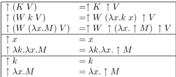
Figure 13: Reduction rules of λf_CPS We can now project λF

CPSonto λ f

↑ (K V ) =↑ K ↑ V ↑ (W k V ) =↑ W (λx.k x) ↑ V ↑ (W (λx.M ) V ) =↑ W ↑ (λx. ↑ M ) ↑ V ↑ x = x ↑ λk.λx.M = λk.λx. ↑ M ↑ k = k ↑ λx.M = λx. ↑ M Figure 14: Projection of λF CPSonto λ f CPS

Remark 19 Note that, in λF

CPS, ↑ M −→ηV2 M, ↑ V −→ηV2 V, ↑ K −→ηV2

Kand if M , V , K are in λfCPS then ↑ M = M , ↑ V = V , ↑ K = K.

Theorem 20 (Galois connection from λf_CPS to λF

CPS) The identity Id_λf CPS

and the mapping ↑ form a Galois connection from λf

CPS, equipped with λ f CPSβη,

to λF

CPS, equipped with λFCPSβη, (and also with only λfCPSβ and λ F CPSβ).

Proof: Given Remark 19, it suffices to check the simulations. • For the simulation of λF

CPSβη by λ f

CPSβη through ↑, we use a

straight-forward induction on the derivation of the reduction step, using the following fact: ↑ M {x =↑ V } =↑ M {x = V } ↑ M {k =↑ K} −→∗ βV1↑ M {k = K} ↑ W {x =↑ V } =↑ W {x = V } ↑ W {k =↑ K} −→∗ βV1 ↑ W {k = K} ↑ K′_{{x =↑ V } =↑ K}′_{{x = V } ↑ K}′_{{k =↑ K} −→}∗ βV1↑ K ′_{{k = K}} ↑ M {k =↑ λx.k x} −→∗βV1↑ M ↑ W {k =↑ λx.k x} −→∗ βV1↑ W ↑ K′_{{k =↑ λx.k x} −→}∗ βV1↑ K ′

• The fact that βV1, βV2, ηV1, ηV2 simulate βV1, βV3, ηV3 through Id

λf_CPS is straightforward. ✷ Corollary 21 (Confluence of λfCPS) λ f CPSβ and λ f CPSβη are confluent.

Proof: By Theorem 20 and Theorem 1. ✷

5.3

From λ

to λ

Definition 7 (The Fischer reverse translation) We now encode λf_CPS into λQ.

(k V )back = [Vback] ((λx.M ) V )back _{= C}

3(Vback, x.Mback)

(y (λx.M ) V )back = y(Vback_{, x.M}back₎

((λk.λz.N ) (λx.M ) V )back = C3(λz.Nback, y.y(Vback, x.Mback))

xback _{= x} (λk.λx.M )back = λx.Mback Lemma 22 1. C2(V back , x.Wback ) −→∗ λQ (W {x = V }) back and C2(V back , x.Mback ) −→∗ λQ (M {x = V }) back . 2. C3(Mback, x.Nback) −→∗_λQ (M {k = λx.N }) back (if k ∈ FV(M)). Proof: By induction on W , M . ✷

Theorem 23 (Simulation of λf_CPS in λQ)

The reduction relation −→_λf

CPSβ is simulated by −→λQ through (_)

back

. Proof: By induction on the derivation of the reduction step, using Lemma 22.

✷

Lemma 24 (Composition of the encodings) 1. V −→∗ λCβ V †back _{and M −→}∗ λCβ (M : k) back . 2. V = Vback † and M = Mback : k.

Proof: By structural induction, using Lemma 22 for the first point. ✷ Now we can prove the following:

Theorem 25 (The refined Fischer translation is a reflection) The refined Fischer translation and (_)back

form a reflection in λQ of λfCPS

(equipped with λf CPSβ).

Proof: This theorem is just the conjunction of Theorem 18, Theorem 23,

and Lemma 24. ✷

Corollary 26 (Confluence of λQ-reductions) λQ is confluent.

Proof: By Theorem 25 and Theorem 1. ✷

6

Connection with Call-by-Value λ-calculus

We have established three connections: • a reflection in λQ of λfCPS,

• a Galois connection from λf_CPS to λF CPS,

• a reflection in λCof λFCPS (in section 3.4).

By composing the first two connections, we have a Galois connection from λQ

to λFCPS, and together with the last one, we have a a pre-Galois connection

from λQto λC. The compositions of these connections also form an equational

correspondence between λQto λC. These facts imply the following theorem:

Theorem 27 (Connections between λQ and λC)

Let us write V♮_{for (↑ (V}F₎₎back _{and M}♯_{for (↑ (M :} Fk))

back

. Let us write V♭_{for (V}†₎F back

and M♭ _{for (M : k)}F back_.

1. For any terms M and N of λC, if M −→λCβ N then M

♯_−→∗ λQ N

♯_.

2. For any terms M and N of λQ, if M −→λQ N then M

♭_−→∗ λCβ N

♭_.

3. For any term M of λC, M ←→∗_λCβ M♯♭.

4. For any term M of λQ, M −→∗λQ M

♭♯_.

Corollary 28 (Equational correspondence between λQ and λC)

1. For any terms M and N of λQ, M ←→∗λQ N if and only if M

♭_←→∗ λCβ

N♭.

2. For any terms M and N of λC, M ←→∗_λ

Cβ N if and only if M

♯_←→∗ λQ

N♯.

We can give the composition of encodings explicitly. We have for instance the following theorem:

Theorem 29 (From λQ to λC) The following equations hold, for the

encod-ing from λQto λC: x♮ _{= x} (λx.M )♮ = λx.M♯ V♯ _{= [V}♮_] (let y = x V in P )♯ = x(V♮_{, y.P}♯₎ (let y = (λx.M ) V in P )♯ = C3(λx.M♯, z.z(V♮, y.P♯))

(let z = V N in P )♯ = (let y = N in (let z = V y in P ))♯ if N is not a value (let z = M N in P )♯ = (let x = M in (let z = x N in P ))♯ if M is not a value (let z = (let x = M in N ) in P )♯ = (let x = M in (let z = N in P ))♯ (let y = V in P )♯ = C3(V♯, y.P♯)

(M N )♯ = (let y = M N in y)♯

Proof: By structural induction, unfolding the definition of the encodings on both sides of each equation. ✷ In fact, we could take this set of equalities as the definition of the direct encoding of λC into λQ. For that it suffices to check that there is a

mea-sure that makes this set of equations a well-founded definition. We now give this measure, given by an encoding of the terms of λCinto first-order terms

equipped with a Lexicographic Path Ordering (LPO) [15].

Definition 8 (An LPO for λC) We encode λC into the first-order syntax

given by the following term constructors and their precedence relation:

ap(_, _) ≻ let(_, _) ≻ ii(_, _) ≻ i(_) ≻ ⋆

The precedence generates a terminating LPO >> as defined in [15]. The en-coding is given in Fig. 15. We can now consider the (terminating) relation induced by >> through the reverse relation of the encoding as a measure for λC.

x = ⋆

λx.M = i(M )

letx = M1M2 inN = let(ii(M1, M2), N )

letx = M in N = let(M , N ) otherwise M N = ap(M , N )

Figure 15: Encoding of λC into the first-order syntax

Remark 30 let(M , N )>>let x = M in N or let(M , N ) = let x = M in N .

Theorem 31 (From λCto λQ) The following properties hold, for the en-coding from λCto λQ: x♭ = x (λx.M )♭ = λx.M♭ C1(V, x.V′)♭ = V′♭{x = V♭} [V ]♭ = V♭ (x(V, y.M ))♭ = let_{y = x V}♭in_M♭ C3(N, x.M )♭ _λCβ∗←− letx = N♭inM♭ C2(V, x.M )♭ = M♭{x = V♭}

Proof: By structural induction, unfolding the definition of the encodings on each side and using Lemma 10. ✷

Remark 32 Note from Theorem 31 and Theorem 29 that if M is a cut-free term of λQ, M♭♯ = M. Also note that we do not have an equality in the

penultimate line but only a reduction. This prevents the use of this theorem as a definition for the encoding from λQto λC, although refining this case (with

different sub-cases) could lead to a situation like that of Theorem 29 (with a measure to find for the set of equations to form a well-formed definition).

The connection between λQ and λC suggests to restricts λC by always

requiring (a series of) application(s) to be explicitly given with a contina-tion, i.e. to refuse a term of λC such as λx.M1 M2 M3 but only accept

λx.let y = M1 M2 M3 iny. The refined Fisher translation of λC, on that

particular fragment, directly has λfCPS as its target calculus, and the

equa-tional correspondence between λCd λQwould then also become a pre-Galois

connection from the former to the latter. The fragment is not stable under rule ηlet, and corresponds to the terms of λCin some notion of ηlet-long normal

form.

This restriction can be formalised with the syntax of a calculus given in [6]:

M, N, P ::= x | λx.M | let x = E in M E ::= M | E M

In fact, this calculus is introduced in [6] as a counterpart, in natural deduction, of a proof-term calculus for an unrestricted sequent calculus (i.e. not specific to the restriction of either LJT or LJQ). The calculus of [6] in natural deduction should thus allow the identification of CBN and CBV reductions as particular sub-reduction systems. Notions corresponding to the restrictions of LJT and LJQ should then capture both the traditional λ-calculus and (the ηlet-long

normal forms of) λC, respectively.

7

Conclusion

In this paper we investigated the call-by-value λ-calculus, and defined continuation-passing-style translations (and their refinements) in the style of Reynolds and Fischer. We have identified the target calculi and proved con-fluence of that of Fischer. We then presented Moggi’s λC-calculus and proved

that a decomposition of its main rule into two steps allowed the refined Fischer translation to form a reflection. Such a decomposition brings λCcloser to the

sequent calculus LJQ.

Indeed, we established new results about LJQ, in connection with Moggi’s λC-calculus. We have introduced a proof-term syntax for LJQ, together with

reduction rules expressing cut-elimination. Such a calculus, called λQ, can be

considered independently from typing and still have a call-by-value semantics given by an adaptation of the Fischer CPS-translation. It relates to λC by

connection. In particular, the reductions in one calculus are simulated by those of the other.

As mentioned in section 4, we leave the proof of strong normalisation of λQfor another paper, since the result pertains to a typed framework and thus

involves some more specific machinery (the typing system was given here to help the intuition about proof-terms).

Further work includes refining the encodings and/or cut-reduction system of λQ, so that the two calculi can be related by a Galois connection or a

reflection.

Another promising direction for further work is given by the calculus from [6] in natural deduction that encompass both the traditional (CBN) λ-calculus and (a minor variant of) the CBV λC-calculus, with a very strong

connection with sequent calculus as a whole (rather than either LJT or LJQ).

References

[1] Jean-Marc Andreoli. Logic programming with focusing proofs in linear logic. J. Logic Comput., 2(3):297–347, 1992.

[2] Vincent Danos, Jean-Baptiste Joinet, and Harold Schellinx. Lkq and lkt: sequent calculi for second order logic based upon dual linear de-compositions of classical implication. In Jean-Yves Girard, Yves Lafont, and Laurent Regnier, editors, Proc. of the Work. on Advances in Lin-ear Logic, volume 222 of London Math. Soc. Lecture Note Ser., pages 211–224. Cambridge University Press, 1995.

[3] R Dyckhoff and C Urban. Strong normalization of Herbelin’s explicit substitution calculus with substitution propagation. J. Logic Comput., 13(5):689–706, 2003.

[4] Roy Dyckhoff and Stéphane Lengrand. LJQ, a strongly focused calcu-lus for intuitionistic logic. In A. Beckmann, U. Berger, B. Loewe, and J. V. Tucker, editors, Proc. of the 2nd Conf. on Computability in Europe (CiE’06), volume 3988 of LNCS, pages 173–185. Springer-Verlag, July 2006.

[5] Roy Dyckhoff and Luis Pinto. Cut-elimination and a permutation-free sequent calculus for intuitionistic logic. Studia Logica, 60(1):107–118, 1998.

[6] José Espírito Santo. Unity in structural proof theory and structural extensions of the λ-calculus. Manuscript, July 2005.

[7] Michael J. Fischer. Lambda calculus schemata. In Proc. of the ACM Conf. on Proving Assertions about Programs, pages 104–109. SIGPLAN Notices, Vol. 7, No 1 and SIGACT News, No 14, January 1972.

[8] Michael J. Fischer. Lambda-calculus schemata. LISP and Symbolic Com-putation, 6(3/4):259–288, December 1993.

[9] Thérèse Hardin. Résultats de confluence pour les règles fortes de la logique combinatoire catégorique et liens avec les lambda-calculs. Thèse de doc-torat, Université de Paris VII, 1987.

[10] H. Herbelin. Séquents qu’on calcule. Thèse de doctorat, Université Paris VII, 1995.

[11] Hugo Herbelin. A lambda-calculus structure isomorphic to Gentzen-style sequent calculus structure. In Leszek Pacholski and Jerzy Tiuryn, editors, Computer Science Logic, 8th Int. Work. , CSL ’94, volume 933 of LNCS, pages 61–75. Springer-Verlag, September 1994.

[12] J. Hudelmaier. Bounds for Cut Elimination in Intuitionistic Logic. PhD thesis, Universität Tübingen, 1989.

[13] Jörg Hudelmaier. An o(n log n)-space decision procedure for intuitionistic propositional logic. J. Logic Comput., 3(1):63–75, 1993.

[14] J-.B. Joinet. Étude de la Normalisation du Calcul des Séquents Classique à Travers la Logique Linéaire. PhD thesis, University of Paris VII, 1993. [15] Samuel Kamin and Jean-Jacques Lévy. Attempts for generalizing the recursive path orderings. Handwritten paper, University of Illinois, 1980. [16] Austin Melton, David A. Schmidt, and George Strecker. Galois connec-tions and computer science applicaconnec-tions. In David Pitt, Samson Abram-sky, Axel Poigné, and David Rydeheard, editors, Proc. of a Tutorial and Work. on Category Theory and Computer Programming, volume 240 of LNCS, pages 299–312, New York, NY, USA, November 1986. Springer-Verlag.

[17] Dale Miller, Gopalan Nadathur, Frank Pfenning, and Andre Scedrov. Uniform proofs as a foundation for logic programming. Ann. Pure Appl. Logic, 51:125–157, 1991.

[18] Eugenio Moggi. Computational lambda-calculus and monads. Report ECS-LFCS-88-66, University of Edinburgh, Edinburgh, Scotland, Octo-ber 1988.

[19] Eugenio Moggi. Notions of computation and monads. Inform. and Com-put., 93:55–92, 1991.

[20] G. D. Plotkin. Call-by-name, call-by-value and the lambda-calculus. The-oret. Comput. Sci., 1:125–159, 1975.

[21] John C. Reynolds. Definitional interpreters for higher-order programming languages. In Proc. of the ACM annual Conf. , pages 717–740, 1972. [22] John C. Reynolds. The discoveries of continuations. LISP and Symbolic

Computation, 6(3–4):233–247, 1993.

[23] John C. Reynolds. Definitional interpreters for higher-order program-ming languages. Higher-Order and Symbolic Computation, 11(4):363– 397, 1998.

[24] Amr Sabry and Matthias Felleisen. Reasoning about programs in continuation-passing style. Lisp Symb. Comput., 6(3-4):289–360, 1993. [25] Amr Sabry and Philip Wadler. A reflection on call-by-value. ACM Trans.

Program. Lang. Syst., 19(6):916–941, 1997.

[26] Nikolaj Nikolaevic Vorob’ev. A new algorithm for derivability in the constructive propositional calculus. Amer. Math. Soc. Transl., 94(2):37– 71, 1970.