Thesis
For the Degree of Doctor of Science In
COMPUTER SCIENCE
By
Barkahoum KADA
Fault-Tolerance and Scheduling in
Embedded Real-Time Systems
Under the Supervision of: Prof. Hamoudi KALLA
Committee members:
Dr. Hocine Riadh
President
University of Batna2
Dr. Houassi Hichem
Examiner
University of Khenchela
Dr. Maarouk Toufik
Messaoud
Examiner
University of Khenchela
Prof. Kalla Hamoudi
Supervisor
University of Batna2
University of Batna 2
Faculty of Mathematics and Computer
Science
ii
First and foremost, I would like to thank Allah almighty for giving me the strength, knowledge, ability, and opportunity to accomplish this thesis. Praise be to Allah. I am deeply grateful to Prof. Hamoudi Kalla, my supervisor, for his constant support, guidance and kindness during this research. This work would not have been possible without his guidance and involvement, his support, and encouragement on daily basis from the beginning till this moment. I am thankful to him for having long discussions with me and giving me invaluable suggestions which helped me to grow my understanding. I deeply express my gratitude and thank him for his support and concern.
I am happy to acknowledge my deepest sincere gratitude to Dr. Riadh Hocine for the honor that he makes to preside this jury. I also thank the members of the thesis committee: Dr. Hichem Houassi and Dr. Toufik Messaoud Maarouk for having accepted to assess my thesis.
A special thanks to my family. I deeply owe it to my parents, who motivated and helped me at every stage of my life.
I owe thanks to a special person, my husband, for his continued and unfailing love, support, and understanding during my pursuit of a Ph.D. degree that made the completion of this thesis possible. He was always there with me in the moments when there was no one to solve my difficulties. I greatly value his contribution and deeply appreciate his belief in me. Last but not the least, I appreciate my daughter and my son, for the long lasting patience and understanding they’re shown during the entire Ph.D. work and thesis writing.
iii
Recently, fault tolerance and energy consumption have attracted a lot of interest in the design of modern embedded real-time systems. Fault tolerance is fundamental for these systems to satisfy their real-time constraints even in the presence of faults and is needed because it is practically impossible to build a perfect system. Transient faults are the most common, and their number is dramatically increasing due to the high complexity, smaller transistors sizes, higher operational frequency, and lowering voltages. Dynamic voltage and frequency scaling (DVFS) is an energy saving technology enabled on most current processors.
This work addresses the issue of fault-tolerant scheduling with energy minimization for hard real-time embedded systems. Our first proposition is an efficient fault tolerance approach that combines two well-known methods: active replication and checkpointing with rollback. Based on this approach we have proposed two algorithms. Static Fault-Tolerant Scheduling algorithm SFTS that explores hardware resources and timing constraints to tolerate multiple transient fault occurrences with respect to hard real-time constraints of precedence-constrained applications. Dynamic Voltage and Frequency Scaling Fault-tolerant Scheduling algorithm DVFS-FTS is proposed to satisfy real-time constraints and to achieve more energy saving even in the presence of faults by adapting the DVFS technique. According to the simulation results, the proposed algorithms have been shown to be very promising for emerging systems and applications where timeliness, fault tolerance, and energy reduction need to be simultaneously addressed.
Keywords: Fault Tolerance, Transient Faults, Checkpointing, Active Replication, Dynamic
iv
Récemment, la tolérance aux fautes et la consommation d’énergie ont attiré beaucoup d’intérêt dans la conception des systèmes temps-réel embarqués modernes.
La tolérance aux fautes est fondamentale pour ces systèmes pour satisfaire leurs contraintes temps-réel même en présence de fautes et elle est nécessaire car il est pratiquement impossible de construire un système parfait. Les fautes transitoires sont les plus courants et leur nombre augmente considérablement en raison de la complexité élevée, des tailles de transistors plus petites, fréquence de fonctionnement plus élevée et des tensions abaissées. DVFS est une technologie de minimisation d’énergie activée sur la plupart des processeurs actuels.
Ce travail traite le problème d’ordonnancement tolérant aux fautes avec minimisation d’énergie pour les systèmes temps-réel embarqués critiques. Notre première proposition est une approche efficace de tolérance aux fautes qui combine les deux techniques : réplication active et checkpointing. En se basant sur cette approche, nous avons proposé deux algorithmes. L’algorithme d’ordonnancement tolérant aux fautes SFTS qui explore l’architecture matérielle et les contraintes temporelles pour tolérer multiples fautes transitoires en respectant les contraintes temps-réel critiques des applications avec contraintes de précédences. L’algorithme d’ordonnancement tolérant aux fautes DVFS-FTS est proposé pour satisfaire les contraintes temporelles et minimiser la consommation d’énergie même en présence de fautes en adaptant la technique DVFS. Selon les résultats de simulation, les algorithmes proposés se sont révélés très prometteurs pour les applications où le respect des contraintes temporelles, la tolérance aux fautes et la minimisation d’énergie doivent être traitées simultanément.
Mots Clés: Tolérance aux Fautes, Fautes Transitoires, Checkpointing, Réplication Active,
v
م
ـــ
خل
ــــــ
ص
مامتهلاا نم ريثكلا ةقاطلا كلاهتساو أطخلا عم حماستلا بذتجا ةريخلأا ةنولآا يف يف ةمظنأ ميمصت ةثيدحلا ةجمدملا يقيقحلا تقولا . تقولا دويق ةيبلتل ةمظنلأا هذهل اًيساسأ اًرمأ أطخلا عم حماستلا دعي لأا دوجو ةلاح يف ىتح يلعفلا اطخ لا نم هنلأ ةيرورض يهو يلاثم ماظن انب ايلمع ليحتسم . ربتعت لأا اطخ يلاعلا ديقعتلا ببسب ريبك لكشب اهددع دادزيو اًعويش رثكلأا يه ةرباعلا ماجحأ ، رغصلأا تاروتسزنارتلا ، ةضفخنملا دوهجلاو يلاعلا ليغشتلا ددرت . يكيمانيدلا ددرتلاو دهجلا سايقم (DVFS) يف اهنيكمت متي ةقاطلل ةرفوم ةينقت وه ةيلاحلا تاجلاعملا مظعم . جلاعي ليلقت عم اطخلأا عم ةحماستملا ةلودجلا ةلأسم لمعلا اذه يقيقحلا تقولا ةمظنلأ ةقاطلا كلاهتسا ةجمدملا . نيتفورعم نيتقيرط نيب عمجي أطخلا عم حماستلل لاعف جهن وه لولأا انحارتقا : طشنلا خسنلا عجارتلا عم شيتفتلا طاقنو . نلا اذه ىلع ً انب نيتيمزراوخ انحرتقا جه . أطخلل ةحماستم ةلودج ةيمزراوخ SFTS عم ةددعتملا ةيلاقتنلاا اطخلأا عم حماستلل ةمزلالا ةينمزلا دويقلاو تادعملا لكيه فشكتست ةيقبسلأا ةديقملا تاقيبطتلل ةجرحلا يقيقحلا تقولا دويق مارتحا . و اطخلأل ةحماستملا ةلودجلا ةيمزراوخ DVFS-FTS بلتل فييكت للاخ نم اطخأ دوجو ةلاح يف ىتح ةقاطلا كلاهتسا ليلقتو تقولا دويق ةي ةينقت DVFS . متي ثيح تاقيبطتلل اًدج ةدعاو ةحرتقملا تايمزراوخلا نأ تبث دقف ةاكاحملا جئاتنل اًقفو دحاو تقو يف ةقاطلا ليلقتو اطخلأا عم حماستلا ، تقولا قيض مارتحا .يحاتفملا تاــــــملكلا
ةــــــ
: أطخلا عم حماستلا ةرباع اطخأ ، شيتفتلا طاقن ، Checkpointing ، طشنلا لثامتملا خسنلا Replication Active يكيمانيدلا دهجلا ددرت سايقم ، ( DVFS ) ليلقت ، ةقاطلا كلاهتسا .vi Acknowledgement ... ii Abstract ... iii List of Figures ... ix List of Tables ... xi Abbreviations ... xii
List of symbols ... xiii
CHAPTER 1General Introduction ... 1
1.1. Context ... 1
1.2. Contributions ... 3
1.3. Thesis organization ... 3
CHAPTER 2Real-Time Systems ... 5
2.1. Introduction ... 5
2.2. Definition ... 5
2.3. Classfication of real-time systems: ... 6
2.3.1. Hard real-time system: ... 7
2.3.2. Soft real-time system: ... 7
2.3.3. Mixed critical system: ... 7
2.4. Real-time task: ... 7
2.4.1. Real-time task characteristics:... 7
2.4.2. States of real-time task... 9
2.4.3. Types of real-time tasks ... 9
2.4.4. Precedence Constraints and Dependencies ... 10
2.4.5. Makespan ... 11
2.5. Real-time scheduling classification... 11
2.5.1. Uniprocessor/Multiprocessor: ... 11
2.5.2. Off-line/On-line: ... 11
2.5.3. Preemptive/Non-Preemptive: ... 12
2.5.4. Static/Dynamic priorities: ... 12
2.5.5. Feasibility and optimality: ... 12
2.6. Embedded Systems ... 13
2.6.1. Definition1 ... 13
vii
2.6.5. Characteristics of Embedded Systems ... 16
2.7. Conclusion ... 17
CHAPTER 3Dependability and Fault Tolerance ... 18
3.1. Introduction ... 18 3.2. Dependability ... 18 3.2.1. Dependability attributes: ... 19 3.2.2. Dependability impairments: ... 20 3.2.3. Dependability means: ... 23 3.3. Fault tolerance:... 25
3.3.1. Fault tolerance techniques ... 25
3.3.2. Error detection techniques ... 26
3.3.3. Redundancy for fault tolerance ... 27
3.4. Conclusion ... 30
CHAPTER 4Literature review ... 32
4.1. Introduction ... 32
4.2. Real-time uniprocessor scheduling ... 32
4.2.1. Rate Monotic RM ... 33
4.2.2. Deadline Monotic DM ... 33
4.2.3. Earliest Deadline First EDF ... 34
4.3. Real-time multiprocessor scheduling ... 35
4.3.1. Related work on real-time multiprocessor scheduling ... 35
4.4. Related work on fault tolerant real-time scheduling ... 38
4.5. Related work on fault-tolerant scheduling with energy minimization ... 40
4.6. Conclusion ... 42
CHAPTER 5A Fault-Tolerant Scheduling Algorithm Based on Checkpointing and Redundancy for Distributed Real Time Systems ... 43
5.1. Introduction ... 43 5.2. Literature review ... 44 5.3. System model ... 46 5.3.1. Application model ... 46 5.3.2. Hardware model ... 47 5.3.3. Fault model ... 47
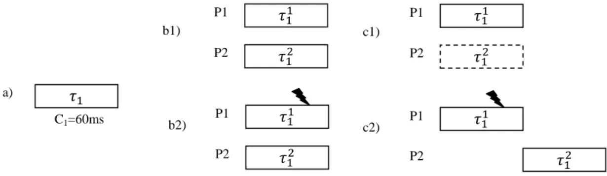
viii
5.4.2. Active replication with checkpointing ... 50
5.5. Motivational example... 53
5.6. The proposed fault tolerant scheduling algorithm ... 54
5.7. Experimental results ... 56
5.8. Conclusion ... 59
CHAPTER 6An Efficient Fault-Tolerant Scheduling Approach with Energy Minimization for Hard Real-Time Embedded Systems... 60
6.1. Introduction ... 60 6.2. Related work... 61 6.3. System models... 62 6.3.1. Application model ... 62 6.3.2. Scheduling model ... 62 6.3.3 Fault model ... 62
6.3.4. Platform and Energy model ... 63
6.4. The fault-tolerance approach ... 64
6.4.1. Uniform Checkpointing with Rollback Recovery ... 64
6.4.2. Collaborative active replication ... 64
6.5. DVFS based fault-tolerance approach ... 66
6.5.1. Optimal frequency assignments ... 67
6.6. The proposed DVFS fault-tolerant scheduling algorithm ... 68
6.7. Performance evaluation ... 70
6.7.1. Simulation parameters ... 70
6.7.2. Experiment results ... 71
6.8. Conclusion ... 72
CHAPTER 7Conclusion and Future Work ... 74
Future work ... 75
ix
List of Figures
Figure 2-1 Real-time system ...6
Figure 2-2 Real-time task parameters ...8
Figure 2-3 Different states of a real-time task [Qamhieh 2015] ...9
Figure 2-4 Precedence constraints example ...11
Figure 2-5 Classification of real-time scheduling ...13
Figure 2-5 Examples of embedded systems ...14
Figure 2-5 Parallel architecture ...15
Figure 2-5 Distributed architecture ...15
Figure 2-6 Example of multiprocessor architecture...16
Figure 3-1 Dependability characteristics ...19
Figure 3-2 Dependability impairments ...20
Figure 3-3 Fault classes [Avizienis et al. 2004] ...23
Figure 3-4 Fault tolerance techniques ...26
Figure 3-5 Different types of redundancy in real-time systems ...28
Figure 3-6 Active redundancy b) and Passive redundancy c) ...29
Figure 4-1 Example of scheduling with Rate Monotic ...33
Figure 4-2 Example of scheduling with DM ...34
Figure 4-3 Example of scheduling with EDF ...35
Figure 4-4 Partitioned Scheduling vs Global Scheduling [Zahaf 2016] ...37
Figure 5 -1 Hard real time application example ...46
Figure 5-2 Hardware example ...47
Figure 5-3 Checkpointing with rollback recovery ...50
Figure 5-4 Scheduling of on virtual processor P# ...51
Figure 5-5 Fault-free scenario ...51
Figure 5-6 Fault occurrence scenario ...52
Figure 5-7 An application example A2 to be scheduled on P1 and P2 under k=2 faults ...53
Figure 5-8 Fault tolerant scheduling: combination of checkpointing with rollback for tasks , and active replication with checkpointing for the task ...54
Figure 5-9 The proposed static fault tolerant scheduling algorithm SFTS ...55
x
Figure 5-12 Feasibility rate of SFTS by doubling fault arrival rate (λ) ...58
Figure 6-1 Illustration of different steps of collaborative active replication ...66
Figure 6-2 The proposed DVFS_FTS algorithm ...69
Figure 6-3 The impact of number of faults on energy saving ...71
Figure 6-4 The impact of application size on energy saving considering k=3 faults ...72
xi
Table 3-1. Comparison between three approaches of redundancy ...30
Table 4-1. Example of Rate Monotic: task set details ...33
Table 4-2. Example of Deadline Monotic: task set details ...34
Table 4-3. Summary of fault-tolerant scheduling ...39
Table 4-4. Summary of fault-tolerant scheduling with energy minimization ...41
Table 5-1. Simulation parameters ...56
Table 5-2. Fault tolerance overheads due to SFTS for different number of faults ...57
Table 5-3. Timing overhead of SFTS compared with checkpoint considering various checkpoint parameters ...58
xii
EDF Earliest Deadline First NFT Non Fault Tolerant
SFTS Static Fault-Tolerant Scheduling Algorithm DVFS Dynamic Voltage and Frequency Scaling
DVFS-FTS DVFS Fault-Tolerant Scheduling Algorithm CH Checkpointing
DAG Directed Acyclic Graph
EXH_FTS Exhaustion Fault-Tolerant Scheduling Algorithm
DVFS_CH DVFS Fault-Tolerant Scheduling Algorithm with Checkpointing ES Energy Saving
DPM Dynamic Power Management ABS Anti-lock Braking System RM Rate Monotic
DMDeadline Monotic RT Real-Time
LLF least laxity First
WCRT Worst Case Execution Time WCCT Worst Case Communication Time TReady Ready List
xiii Notation Definition
The ith task in the task set = { / i = 1...n}
Ci The worst execution time of in a fault free condition
Di The deadline of the task
Ui The utilization of the task
eij Data dependency between and
Pj The jth processor in the set of processors Ρ = {Pj / j=1…M}.
K Number of transient faults
λ Failure rate
The criticality threshold
mi Number of checkpoints for the task
Ci(mi) The fault free execution time of the task using checkpointing Oi The time overhead for the task for saving one checkpoint
Ri(mi)
The recovery time of the task with mi checkpoints under one
fault
ri
The time overhead for the task to rollback to the latest checkpoint
WCRTi
The worst case response time of the task in the presence of
K faults
The jth segment of the task
The jth replica of the task P# Virtual processor.
STi The start time of the task
FTi The finish time of the task
Checkpoint saving
µ Recovery cost
Effective deadline of the task Optimal Frequency
xiv
Effective Loading Capacitance
Supply Voltage Power Consumption Static Power
Constant independent of operating frequency Dynamic Power
Energy Consumption
1
CHAPTER 1
General Introduction
1.1. Context
With the rapid growth in technology, the contemporary computing systems available in today's era are shrinking in size and weight, exhibiting high performance and are capable of communicating with each other over the network. This has made embedded systems common place in everyday life. Unlike general purpose systems, embedded systems receive input from different sources through sensors and provide output to different devices through actuators without human intervention. These systems are used in many diverse application areas namely, automated industry applications, automotive applications, avionics, defense applications, consumer electronics etc. Many of the embedded systems are specially made for performing real-time tasks where the timing constraints are important. Such systems are known as real-time embedded systems. For example, in a missile guided system, the highly critical hard real-time tasks like target sensing and track correction require an independent system mounted on the missile to sense the target and correct the path of the missile. If these tasks are not completed in time, the missile may home onto unwanted area and cause disaster [Digalwar 2016].
Based on the cost of failure associated with not meeting timing constraints, real-time systems can be classified broadly as either hard or soft. A hard real-time constraint is one whose violation can lead to disastrous consequences such as loss of life or a significant loss to property as a missile guided system. In contrast, a soft real-time constraint is less critical; hence, soft real-time constraints can be violated. However, such violations are not desirable, either, as they may lead to degraded quality of service, and it is often the case that the extent of violation be bounded. Multimedia system is an example of system with soft real-time constraints.
Fault tolerance is fundamental for real-time systems to satisfy their real-time constraints even in the presence of faults. As shown in [Srinivasan et al. 2003], processor faults can be broadly
2
classified into two categories: transient and permanent faults. Transient faults are the most common, and their number is dramatically increasing due to the high complexity, smaller transistors sizes, higher operational frequency, and lowering voltages [Djosic and Jevtic 2013, Salehi et al. 2016, Li et al. 2015, Krishna 2014]. They may cause errors in computation and corruption in data, but are not persistent. On the other hand, permanent faults, also called hard errors can cause hardware damages to processors and bring them to halt permanently.
Fault tolerance is essentially based on redundancy. In literature [Dubrova 2013, Motaghi and Zarandi 2014, Zhang and Chakrabarty 2006, Izosim et al, 2008], two families of redundancy are used in fault tolerant scheduling of real-time systems: spatial redundancy and
time-based redundancy. Spatial redundancy is effective to tolerate multiple spatial faults
(permanent or transient) and is more preferable for safety-critical systems. However, it is very costly and can be used only if the amount of resources is virtually unlimited [Pop et al. 2009]. In order to reduce cost, other techniques are required such as recovery with checkpointing and re-execution which are classified by Motaghi and Zarandi (2014) time-based redundancy. However these techniques introduce significant time overheads, where the non respect of time-constraint can lead to unschedulable solution. Therefore, the design of an efficient fault-tolerant approach is required to meet time and cost constraints of embedded systems.
Dynamic power/energy management is an active area of research in the design of embedded real-time systems. Extensive power management techniques [Tavana et al. 2014, Li et al. 2011, Gupta 2004, Hu et al. 2016, Han et al. 2015] have been developed on energy minimization for real-time systems under a large diversity of system and task models [Mahmood et al. 2017, Wei et al. 2012]. Among these techniques, Dynamic Voltage and Frequency Scaling (DVFS) is one of the most popular and widely deployed schemes. Most modern processors, if not all, are equipped with DVFS capabilities. DVFS dynamically adjusts the supply voltage and working frequency of a process to reduce power consumption at the cost of extended circuit delay.
The real-time scheduling on multiprocessor system with only the timing constraints has been identified as a NP-hard problem [Shin and Ramanathan 1994]. In addition of the two criteria: reliability and energy consumption makes the real-time scheduling problem even hard to study.
3
1.2. Contributions
In this thesis, we will be interested in fault-tolerant scheduling with energy minimization of hard real-time tasks with precedence constraints in multiprocessor platform. Thus, the main contributions of this thesis are:
We design an efficient fault-tolerant scheduling approach that explores hardware resources and timing constraints. This approach combines two well-known policies: checkpointing with rollback and active replication. Replicas collaboration is introduced to tolerate spatially or temporally faults and satisfy critical task constraint. To the best of our knowledge, this is the first work introducing the idea of collaboration between replicas in active replication technique with checkpointing. The proposed approach classifies the real-time tasks into critical and noncritical ones, according to the utilization of the task. For the non critical task, we adopt checkpointing with rollback technique to tolerate multiple transient faults. Whereas for the critical task, we adopt active replication as it is the fault-tolerant method that explores hardware resources to meet timing constraints and provide high reliability even when deadlines are tight.
Based on the explained fault-tolerance approach, we have proposed a fault-tolerant scheduling algorithm SFTS which can tolerate K transient faults.
We investigate the energy minimization problem for fault-tolerant scheduling of hard real-time systems. We extend the proposed fault-tolerance approach to incorporate it with DVFS to exploit the released slack time for energy saving. DVFS is used during uniform checkpointing with rollback technique. However, with active replication, task replicas must be performed at the maximum frequency given the probability of failure is low.
An efficient fault-tolerant scheduling heuristic DVFS_FTS based on the Earliest-Deadline-First (EDF) algorithm is presented to minimize energy consumption while tolerating K transient Faults.
1.3. Thesis organization
4
Chapter 2 introduces the basic concepts of real-time system and embedded system. It
presents their characteristics, architectures and the classification of real-time scheduling.
Chapter 3 provides in the first part an overview of dependability characteristics (attributes,
impairments and means) and the different classes of faults. The second part is dedicated to our principle aim: fault tolerance. We present their different techniques and the principle classes of redundancy in real-time systems (spatial redundancy and time-based redundancy).
Chapter 4 provides an overview of related work on multiprocessor scheduling, fault
tolerance, and energy consumption in embedded real-time systems. Chapters 5 and 6 are devoted to the main contributions of this dissertation
Chapter 5 focuses on the choice of fault-tolerant mechanisms that ensure our system
reliability. It starts with a general description of our system model (Application, Architecture, and fault model). Then, we concentrate on describing our fault tolerance approach based on active replication and uniform checkpointing with rollback. After, we exploit this approach in the first proposed fault-tolerant scheduling algorithm SFTS. Finally, simulation results are given to prove the performance of the proposed algorithm.
Chapter 6 is dedicated to another challenge of real-time embedded systems: energy minimization. We extend the proposed fault-tolerance approach in chapter 5 to incorporate it
with DVFS to achieve more energy saving. Then, we present the fault tolerant scheduling algorithm DVFS_FTS developed for reducing dynamic energy. Finally, Experiment results have shown that the proposed algorithm achieves a considerable amount of energy saving compared to others algorithms.
Chapter 7 concludes the thesis by discussing the overall contribution of the research. In
5
Real-Time Systems
2.1. Introduction
The distinguishing characteristic of a real-time system in comparison to a non-real-time system is the inclusion of timing requirements in its specification. That is, the correctness of a real-time system depends not only on logically correct segments of code that produce logically correct results, but also on executing the code segments and producing correct results within specific time frames. Thus, a real-time system is often said to possess dual notions of correctness, logical and temporal.
In this chapter, we present first the basic concepts of real-time systems and their classification. Then, we provide classes of real-time scheduling. We focus in this thesis on real-time embedded systems. Finally, we describe some basic concepts pertain to embedded systems.
2.2. Definition
The Oxford dictionary defines real-time as “the actual time during which a process or event
occurs”. In computer science, real-time systems are defined by Burns and Wellings (2001)
“those systems in which the correctness of the system depends not only on the correctness of
logical result of computation, but also on the time on which results are produced”. The
validity of a real-time system depends not only on the results of the processing performed but also on the temporal aspect.
Recently, the term real-time is widely used to describe many applications and computing systems that are somehow related to time, such as real-time trackers, gaming systems and information services. The following list contains certain examples of practical real-time applications:
6
Multimedia and entertainment systems: multimedia information is in the form of streaming audio and video.
Data distribution systems which notify users of important information in a short delay (few minutes or less). Such systems are found mainly in transport systems to inform passengers of accidents and schedule delays or changes.
General purpose computing such as in financial and banking systems.
Medical systems such as peacemakers and medical monitors of treatments or surgical procedures.
Industrial automation systems such as the ones found in factories to control and monitor production process. For example, sensors collect parameters periodically and send them to real-time controllers, which evaluate the parameters and modify processes when necessary. These systems can handle non-critical activities as in logging and surveillance.
General control management systems such as the ones found in avionic systems. Real-time engine controllers are responsible of automatic navigation and detection of hardware malfunctions or damages through reading sensors and processing their parameters and react within an acceptable delay.
Figure 2-1 Real-time system
2.3. Classfication of real-time
systems:
Depending on the criticality of the timing constraints, three categories of real-time system can be distinguished:
Real-time
system Environment (e.g. production
process)
Data, measures, events
7
2.3.1. Hard real-time system:
The correctness of their outputs depends on respecting given timing constraints or catastrophic results occur. If such systems fail in performing their tasks within acceptable deadline margins, their results become useless and might lead to catastrophic consequences. It’s a system subject to strict timing constraints, that is to say for which the slightest temporal error can have catastrophic human or economic consequences. Air traffic control systems and nuclear station control systems are real-time strict.
2.3.2. Soft real-time system:
Soft real-time systems have flexible timing constraints and they perform less critical activities and tasks. The quality of services provided by soft real-time systems depends on providing results within a minimum delay. If such delay is not respected, the quality degrades but not the correctness of the execution or results.
2.3.3. Mixed critical system:
They are defined by [Saraswat et al. 2010] and [Izosimov 2008] the systems with tasks of different levels of time-criticality, for example running hard real-time and soft real-time tasks in the same system.
2.4. Real-time task:
A real-time task is a sequence of instructions that is the basic unit of a real-time system. The tasks perform inputs / outputs and calculations to control processes via a set of sensors and actuators, possibly all or nothing, for example set of tasks performing the speed controller of a car or the automatic control of a plane.
2.4.1. Real-time task characteristics:
A real-time application is composed of a set of n tasks denoted by , where . Generally, a real-time task is described by the following parameters (all these
8
Ri (Ready time or Release time): it is the time on which the task can begin its
execution;
STi (Start time), FTi (End time): are respectively the time on which the task is
executed on the processor also called the start time of execution and the time on which the task finishes its execution also called the end time of execution;
RTi (Response time): it represents FTi -Ri;
WCRT (Worst Case Response time) Ci: which is an estimation of the longest possible
execution time of any task , i.e., the actual execution time of a task should never exceed its WCRT in any scenario. The evaluation of WCRT of tasks is very important for the reliability of real-time systems to be valid, the value of this parameter must not be overestimated too much, must be safe (never overestimated) and the pessimism of their estimations increases relatively to the criticality of the application [Qamhieh 2015];
Di (Deadline): which is the time interval in which each task executes with respect to
its release time. In hard real-time systems, any task must always meet their deadline, whereas execution tardiness of task is accepted in soft real-time systems. Two types of deadlines exist:
Relative Di: the time interval between the start of the task and the completion of
the real-time task is known as relative deadline. It is basically the time interval between arrival and corresponding deadline of the real-time task.
Absolute Di +Ri: the time within which execution of a task should be
completed.
Li (Laxity): this is the largest time for which the scheduler can safely delay the task
execution before running it without any interruption.
Ti (Period): which is the minimum inter-arrival time between two releases of the same
task.
Figure 2-2 Real-time task parameters
Ci Di STi FTi Ri time RTi Di +Ri
9
The processor utilization of task is defined as the task’s processor usage and it is denoted
by . The utilization of a task set is the sum of utilization of its tasks, where
2.4.2. States of real-time task
The main objective of a real-time scheduler is to guarantee the correctness of the results while respecting the timing constraints of the tasks (no deadline miss).
Based on the decisions of the scheduler, a real-time task can be in one of the following states:
• Ready state: The task is activated and it is available for execution, but it is not
currently selected by the scheduler to execute on a processor.
• Running state: The task is assigned to a processor and it is actually executing.
• Blocked state: if the task is waiting for an event to happen such as an I/O event, it
remains blocked and cannot be scheduled until the event happens. Then the task moves to the ready state.
The different states of tasks are shown in Figure 2-3. Moreover, a real-time scheduler controls the transitions between the ready and running states of tasks, but it has no control over the external events that block the execution of tasks.
Figure 2-3 Different states of a real-time task [Qamhieh 2015]
2.4.3. Types of real-time tasks
There exist three types of real-time tasks:
RT Scheduler Blocked Ready Runing resumed event ent Waiting for event preempted activate d
10
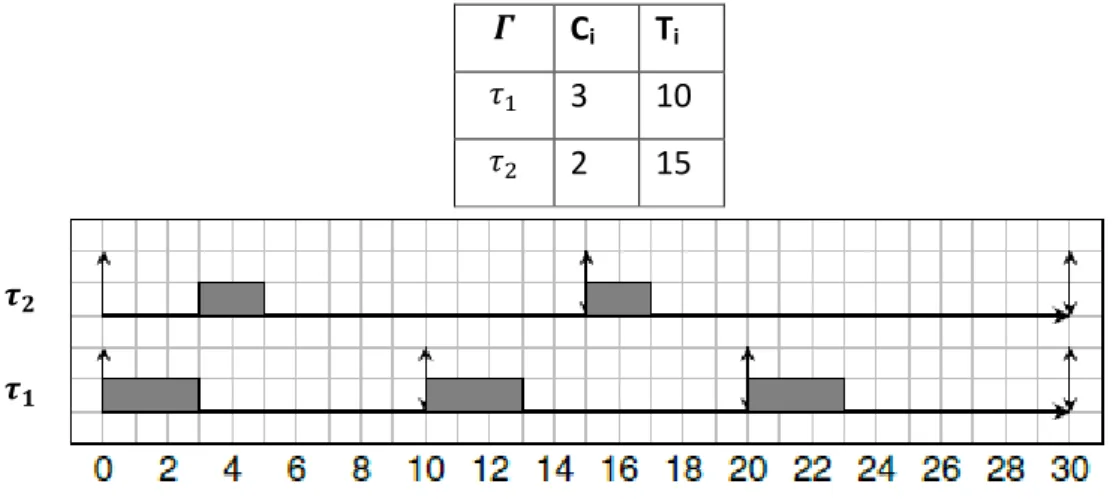
2.4.3.1. Period task:
A task is called periodic if the event that conditions its activation occurs at regular intervals of time (period) Ti and each activation is called instance.
2.4.3.2. Aperiodic task:
The activation time is random and can not be anticipated, since its execution is determined by the occurrence of an internal event (for example the arrival of a message) or an external event (e.g. the requests of the operator). Anti-lock Braking System (ABS) in modern cars is a typical system that employs aperiodic real-time tasks.
2.4.3.3. Sporadic task:
It's a special case of aperiodic tasks where a minimum duration of time separates two successive activations. To take them into account, these tasks are often considered as periodic tasks [Kermia 2009] to apply the existing results of the periodic tasks.
2.4.4. Precedence Constraints and Dependencies
A dependency between two tasks and can be of two types: a precedence dependency
and / or a data dependency. A precedence dependence between means that the task
cannot begin its execution until the task has been completed. Precedence constraints are indirectly real-time constraints and we say that the task is a predecessor of the task and
is a successor of [Forget 2011].
A data dependency between indicates that the task produces a data that is consumed by . This dependence necessarily leads to precedence between the tasks. The tasks are said to be independent when they are defined only by their temporal parameters [Ndoye 2014].
The set of dependencies between the tasks can be modeled by a Directed Acyclic Graph DAG where the nodes represent the tasks and the arcs the dependencies between the tasks. An example of DAG is shown in the Figure 2-4.
11
Figure 2-4 Precedence constraints example
In this thesis, we are interested in hard real-time systems with aperiodic dependant tasks.
2.4.5. Makespan
Reflects the time that elapses between the start date of the first executed task and the finish date of the last executed task. The goal is to develop algorithms which in addition to respecting other time constraints, minimize makespan [Lin and Liao 2008].
2.5. Real-time scheduling
classification
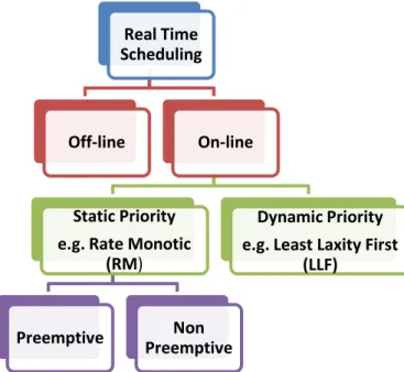
Real-time scheduling is defined as the process that defines the execution order of tasks on processor platforms. There are several classes of real-time scheduling algorithms, we can cite the following classification [Yahiyaoui 2013]:
2.5.1. Uniprocessor/Multiprocessor:
Real-time scheduling is said uniprocessor scheduling if the architecture has only one processor. If multiple processors are available, the scheduling is multiprocessors.
2.5.2. Off-line/On-line:
In off-line scheduling, the schedules for each task need to be determined in advance, therefore it requires prior knowledge of the characteristics of tasks. It only incurs little runtime overhead. In contrast, on-line scheduling calculates the schedules during runtime, hence it can
4
12
provide more flexibility to react to uncertainties of task characteristics at the cost of large runtime overhead.
2.5.3. Preemptive/Non-Preemptive:
A scheduling is preemptive if the execution of any task can be interrupted to requisition the processor for another more urgent or higher priority task. The scheduling is said to be non-preemptive if, once started, the task being executed cannot be interrupted before the end of its execution.
2.5.4. Static/Dynamic priorities:
Most scheduling algorithms are priority-based: they assign priorities to the tasks in the system and these priorities are used to select a task for execution whenever scheduling decisions are made. A scheduling algorithm is called static priority algorithm if there is a unique priority associated with each task. e.g. of such algorithms is Rate Monotic (RM).
A scheduling algorithm has dynamic priorities, if the priorities of the tasks are based on dynamic parameters (for example laxity). e.g. of such category is the Least Laxity First (LLF) scheduling algorithm.
These classes of real-time systems are illustrated in Figure 2-5.
2.5.5. Feasibility and optimality:
A task is referred to as schedulable according to a given scheduling algorithm if its worst-case response time under that scheduling algorithm is less than or equal to its deadline. Similarly, a task set is referred to as schedulable according to a given scheduling algorithm if all of its tasks are schedulable.
A task set is said to be feasible, if there is at least one scheduling algorithm that can schedule the task set while meeting all task deadlines [Legout 2014].
Additionally, a scheduling algorithm is referred as optimal if it can schedule all of the task sets that can be scheduled by any other algorithm. In other words, all of the feasible task sets [Zahaf 2016].
13
Figure 2-5 Classification of real-time scheduling
2.6. Embedded Systems
In this thesis the applications that interest us are real-time and also embedded. This forces us to take into account the properties of these systems in the work that we carry out.
2.6.1. Definition1
An embedded system can be broadly defined as a device that contains tightly coupled hardware and software components to perform a single function, forms part of a larger system, is not intended to be independently programmable by the user, and is expected to work with minimal or no human interaction [Jimenez 2014].
2.6.2. Definition2
An embedded system is a combination of computer hardware and software, and perhaps additional mechanical or other parts, designed to perform a specific function.
Most embedded systems interact directly with processes or the environment, making decisions on the fly, based on their inputs. This makes necessary that the system must be reactive, responding in real-time to process inputs to ensure proper operation. Besides, these
Real Time Scheduling
Off-line On-line
Static Priority e.g. Rate Monotic
(RM)
Preemptive Preemptive Non
Dynamic Priority e.g. Least Laxity First
14
systems operate in constrained environments where memory, computing power, and power supply are limited. Moreover, production requirements,
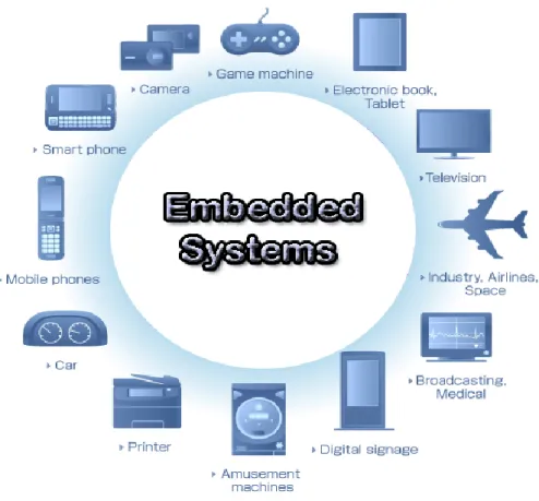
2.6.3. Application of embedded systems
Embedded systems are used in different applications like automobiles, telecommunications, smart cards, missiles, satellites, computer networking and digital consumer electronics (see Figure 2-6).
Figure 2-6 Examples of embedded systems
2.6.4. Embedded system architecture
It consists of a hardware part, which interacts with environment and formed by a set of physical elements: processor(s), memory(s) and inputs/outputs. At the same time, a specific software part which consists of programs and a power source.
Embedded systems sometimes require the use of several processors which can be of different types. A first classification of architectures for embedded systems depends on the number of
15
processors: single-processor or multi-processor architecture. There are different classifications for multiprocessor architectures:
Homogeneous / Heterogeneous in relation to the nature of the processors available to the
architecture:
Homogeneous: In this case the processors are identical .i.e. they are interchangeable and they have the same computing capacity;
Heterogeneous: The processors are either independent .i.e. processors are not intended to perform the same tasks or uniform .i.e. the processors perform the same tasks but each processor has its own computational capacity.
Homogeneous / Heterogeneous depending on the nature of communications between
processors:
Homogeneous: If the communication costs between each pair of processors in the architecture are always the same;
Heterogeneous: If the communication costs between processors vary from one pair of processors to another.
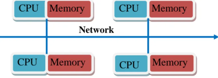
Parallel / Distributed according to the type of memory available to the architecture:
Parallel: This architecture model corresponds to a set of processors communicating by shared memory (see Figure 2-7);
Figure 2-7 Parallel architecture
Distributed: It corresponds to a set of distributed memory processors communicating by messages (see Figure 2-8).
Figure 2-8 Distributed architecture
Shared Memory CPU CPU CPU CPU CPU Memory CPU Memory CPU Memory CPU Memory Network
16
As represented in Figure 2-9, multiprocessor architectures are often represented by a graph where the vertices are the processors. If an arc connects two vertices, this means that these two vertices can communicate directly through the communication medium (bus, memory ...).
Figure 2-9 Example of multiprocessor architecture
2.6.5. Characteristics of Embedded Systems
The design of an embedded system must respect a certain number of characteristics, we list below the most important:
Must be dependable:
Reliability: R(t) = Probability of system working correctly provided that is was working at t=0.
Maintainability: M(d) = Probability of system working correctly d time units after error occurred.
Availability: Probability of system working at time t
Safety: No harm to be caused.
Security: Confidential and authentic communication. Must be efficient:
Energy efficient.
Code-size efficient (especially for systems on a chip).
Run-time efficient.
Weight efficient.
Cost efficient.
Many Embedded System must meet real-time constraints:
Processor1 Processor3 Processor2 Processor4 M M M M
17
A real-time system must react to stimuli from the controlled object (or the operator) within the time interval dictated by the environment.
For real-time systems, right answers arriving too late (or even too early) are wrong.
2.7. Conclusion
We have presented in this chapter real-time and embedded systems, their characteristics, application, and classification. In this thesis, we have considered critical real-time systems, i.e. those which must satisfy the time constraints to prevent the system from the various possible disasters. As the main characteristic of these systems is to be reliable, we will present in the following chapter the basic concepts of fault tolerance and dependability.
18
Dependability and Fault
Tolerance
3.1. Introduction
Fault tolerance is the ability of a system to continue performing its intended function in spite of faults. In a broad sense, fault tolerance is associated with reliability, with successful operation, and with the absence of breakdowns. A fault-tolerant system should be able to handle faults in individual hardware or software components, power failures or other kinds of unexpected disasters and still meet its specification. The ultimate goal of fault tolerance is the development of a dependable system.
The first part of this chapter begins by defining what dependability is. Then, we describe the basic concepts in the field of dependability (attributes, impairments and means) and identify the different classes of faults.
The second part is dedicated to our principle objective: fault tolerance. We present their different techniques and the principle classes of redundancy in real-time systems (spatial redundancy and time-based redundancy).
3.2. Dependability
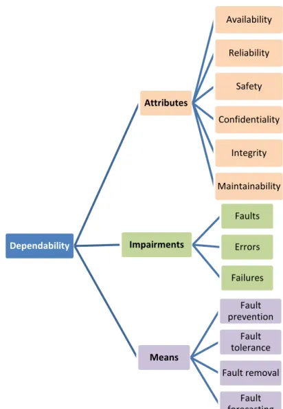
Dependability is the ability of a system to deliver its intended level of service to its users [Krakowiak 2004]. As computer systems become relied upon by society more and more, the dependability of these systems becomes a critical issue. In the next, we present three characteristics of dependability as shown in Figure 3-1: attributes, impairments and means.
19
Figure 3-1Dependability characteristics
3.2.1. Dependability attributes:
The attributes of dependability express the properties which are expected from a system:
Reliability: The ability of the system to deliver its service without interruption.
Safety: The ability of the system to perform its functions correctly or to discontinue its function in a safe manner.
Availability: The proportion of time which system is able to deliver its intended level of service.
Confidentiality: The absence of unauthorized disclosure of information.
Integrity: The absence of inappropriate alterations to information leads to integrity
Maintainability: The ability to undergo modifications and repairs.
Dependability Attributes Availability Reliability Safety Confidentiality Integrity Maintainability Impairments Faults Errors Failures Means Fault prevention Fault tolerance Fault removal Fault forecasting
20
3.2.2. Dependability impairments:
Dependability impairments are usually defined in terms of faults, errors, failures which are linked as illustrated in Figure 3-2. A common feature of the three terms is that they give us a message that something went wrong. A difference is that, in case of a fault, the problem occurred on the physical level; in case of an error, the problem occurred on the computational level; in case of a failure, the problem occurred on a system level.
Figure 3-2 Dependability impairments
3.2.2.1. Fault:
A fault is a physical defect, or flaw that occurs in some hardware or software component. Examples are short-circuit between two adjacent interconnects, broken pin, or a software bug.
Classes of faults
As shown in Figure 3-3, the work done by [Avizienis et al. 2004] classifies all faults according to eight basic viewpoints. Each of these eight classes is called an elementary fault class.
Classification According to Phase of Creation or Occurrence
The lifecycle of a system consists of a development phase and a use phase. The development phase involves all activities that lead to the system being ready to deliver its service for the first time, from the conception of an initial idea, to a specification, to a design, to the manufacturing, and to the final deployment. The use phase involves everything that happens after the system has been deployed and consists of alternating periods of service delivery, service outage and service shutdown (an intentional and authorized interruption of the service). Faults can be introduced into a system during either phase. Faults introduced during the development phase are called development faults. Faults introduced during the use phase are called operational faults.
Classification According to System Boundaries
A system is separated from its environment by a common frontier called the system boundary. Based on this boundary, faults can be classified according to whether they originate within it
Fault Failure Error Fault … … … … … … … … …
21
or outside of it. Faults originating within the system boundary are called internal faults. Faults originating outside of it are called external faults. What exactly is an internal or external fault therefore depends on where we trace the system boundary. The physical deterioration of a component would be an example of an internal fault. The failure of a cooling system that is part of the environment, and whose purpose is to prevent overheating of the system, would be an example of an external fault.
Classification According to the Phenomenological Cause
Another way to classify faults is whether they can be attributed to people or whether they are due to natural phenomena. Using this criterion, we distinguish between human-made faults, which are those for which we can blame a person, and natural faults, which are those for which we will have to blame natural phenomena.
Classification According to Dimension
The dimension of a fault refers to whether it affects hardware or software. In the first case we talk about hardware faults; in the second, we talk about software faults. Examples of hardware faults include the deterioration of physical parts, loose connectors, broken wires, and manufacturing defects. Examples of software faults include typos in source code and incorrectly implemented functions.
Classification According to Objective
Human-made faults, which we saw a moment ago, can be classified according to their objective. In that case we distinguish between malicious and non-malicious faults. Malicious
faults are those that are introduced with the objective to cause harm to the system or its
environment. Non-malicious faults, unsurprisingly, are those introduced without the intent to cause harm. Examples of malicious faults include Trojan horses, trapdoors, viruses, worms, zombies, and wiretapping. Examples of non-malicious faults include any honest mistake when designing, deploying or using a system.
Classification According to Intent
Another way of classifying human-made faults is according to their intent. Here we distinguish between deliberate faults and non-deliberate faults. To decide whether a fault is deliberate or non-deliberate, we basically have to ask the person that just introduced the fault “did you do that on purpose?”. If the answer is yes, we have a deliberate fault; otherwise, we have a non-deliberate fault. An example is when a designer purposely chooses not to add any electromagnetic shielding to reduce the weight or cost of a system. Depending on the
22
electromagnetic harshness of the environment where the system needs to operate, this may be a fault
Classification According to Capability
Avižienis et al. 2004 also classify human-made faults according to the capability (or competence) of the person introducing the fault. Using this criterion we distinguish between accidental faults and incompetence faults. Accidental faults are those introduced inadvertently, presumably due to a lack of attention and not due to a lack of skills; whereas
incompetence faults are those introduced due to a lack of skills. Classification According to Persistence
Finally, Avizienis et al. (2004) classify faults according to their persistence: faults can either be permanent faults, meaning that once present, they do not disappear again without external interventions such as repairs; or they can be transient faults, meaning that they disappear after some time. An example of a permanent fault is a deteriorated component. An example of a transient fault is an electromagnetic interference.
3.2.2.2. Error:
An error is a deviation from correctness or accuracy in computation, which occurs as a result of a fault. Errors are usually associated with incorrect values in the system state. For example, a circuit or a program computed an incorrect value, an incorrect information was received while transmitting data.
3.2.2.3. Failure:
A failure is a non-performance of some action which is due or expected. A system is said to have a failure if the service it delivers to the user deviates from compliance with the system specification for a specified period of time. A system may fail either because it does not act in accordance with the specification, or because the specification did not adequately describe its function.
23
Figure 3-3 Fault classes [Avizienis et al. 2004]
3.2.3. Dependability means:
Dependability means are the methods and techniques enabling the development of a dependable system. Fault tolerance, which is the subject of this thesis, is one of such methods.
Faults
ss Phase of creation Or occurrence System boundaries Phenomenological cause Dimension Hardware faults[Originate in, or affect, hardware]
Software faults
[Affect software, i.e., programs or data]
Intent
Deliberate faults
[Result of a harmful decision]
Non-deliberate faults [Introduced without awareness] Natural faults
[Caused by natural phenomena without human participation] Human-Made faults
[Result from human actions] Internal faults
[Originate inside the system boundary]
External faults
[Originate outside the system boundary and propagate errors into the system by interaction of interference]
Development faults
[Occur during (a) system development, (b) maintenance during the use phase and (c) generation of procedures to operate or to maintain the system] Operational faults
[Occur during service delivery of the use phase]
Objective
Malicious faults
[Introduced by a human with the malicious objective of causing harm to the system] Non-Malicious faults
[Introduced without a malicious objective]
Capability
Accidental faults [Introduced inadvertently] Incompetence faults
[Result from lack of professional competence by the authorized human(s), or from inadequacy of the development organization]
Persistence
Permanent faults
[Presence is assumed to be continuous in time]
Transient faults
24
It is normally used in a combination with other methods to attain dependability, such as fault prevention, fault removal and fault forecasting.
3.2.3.1. Fault prevention:
Fault prevention is attained by quality control techniques employed during the design and manufacturing of hardware and software. They include structured programming, information hiding, modularization, etc., for software, and rigorous design rules for hardware.
3.2.3.2. Fault tolerance:
Fault tolerance is intended to preserve the delivery of correct service in the presence of active faults. Fault tolerance is achieved by using some kind of redundancy.
3.2.3.3. Fault removal:
Fault removal is performed both during the development phase, and during the operational life of a system. Fault removal during the development phase of a system life-cycle consists of three steps: verification, diagnosis, correction. Fault removal during the operational life of a system is corrective or preventive maintenance. Corrective maintenance is aimed at removing faults that have produced one or more errors and have been reported, while
preventive maintenance is aimed to uncover and remove faults before they might cause
errors during normal operation.
3.2.3.4. Fault forecasting:
Fault forecasting is conducted by performing an evaluation of the system behavior with respect to fault occurrence or activation. Evaluation has two aspects:
Qualitative or ordinal evaluation, which aims to identify, classify, rank the failure modes, or the event combinations (component failures or environmental conditions) that would lead to system failures,
Quantitative or probabilistic evaluation, which aims to evaluate in terms of probabilities the extent to which some of the attributes of dependability are satisfied; those attributes are then viewed as measures of dependability.
25
The main objective of this dissertation is fault tolerance in real-time embedded systems. Therefore, the next section elaborates more on fault tolerance in general, and the specific techniques used in this thesis in particular.
3.3. Fault tolerance:
Whatever precautions are taken, the occurrence of faults is inevitable (human error, malicious intent, aging of equipment, natural disaster, etc.). This does not mean that one should not try to prevent or eliminate faults, but the measures taken can only reduce the likelihood of their occurrence. Several techniques of fault tolerance have been proposed, they are all based on redundancy. In the next, we first present fault tolerance techniques and then we describe the different types of redundancy.
3.3.1. Fault tolerance techniques
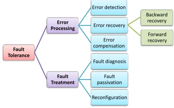
The goal of fault tolerance is to provide a correct system service in spite of faults. As shown in Figure 3-4, Fault tolerance is carried out by error processing and by fault treatment [Derasevic 2018]. Error processing is aimed at removing errors from the computational state, if possible before failure occurrence; fault treatment is aimed at preventing faults from being activated again.
3.3.1.1. Error processing
May be realized by using the following three primitives [Laprie 1995]:
Error detection: It is done by identifying the erroneous state before replacing it with an error-free one
Error recovery: It is done by restoring an error-free state starting from the erroneous state. This can be achieved using two different approaches:
Backward recovery is done by restoring the system to a prior error-free state using the pre-saved points in time, called the recovery points (checkpoints) that were established before the error has occurred.
26
Forward recovery is done by transforming an erroneous state with a new state in which the system may resume to provide its service, but possibly in a degraded mode.
Error compensation: It is done by employing enough redundancy to allow the system to provide its service in spite of the erroneous internal state.
3.3.1.2. Fault treatment
Is accomplished by the execution of two subsequent steps. The first step is called fault
diagnosis and it involves discovering what are the causes of errors covering their location and
nature. The next step is called fault passivation and its aim is to realize the prime goal of fault treatment which is to prevent faults from causing any further errors, i.e. to passivate them. This step is accomplished by excluding the identified faulty components from the rest of the system execution. If this exclusion causes the system not to be able to preserve the delivery of intended service, then a reconfiguration of the system might be realized [Derasevic 2018].
Figure 3-4 Fault tolerance techniques
3.3.2. Error detection techniques
In order to achieve fault tolerance, a first requirement is that faults have to be detected. Researchers have proposed several error detection techniques, including watchdogs, assertions, signatures, duplication, and memory protection codes.
Fault Tolerance Error Processing Error detection Error recovery Error compensation Fault Treatment Fault diagnosis Fault passivation Reconfiguration Backward recovery Forward recovery
27
Signatures [Oh et al. 2002a, Nicolescu et al. 2004]: Are among the most powerful error
detection techniques. In this technique, a set of logic operations can be assigned with precomputed “check symbols” (or “checksum”) that indicate whether a fault has happened during those logic operations. Signatures can be implemented either in hardware, as a parallel test unit, or in software. Both hardware and software signatures can be systematically applied without knowledge of implementation details.
Watchdogs: In the case of watchdogs [Benso et al. 2003, Kalla 2004, Bachir 2019], program
flow or transmitted data is periodically checked for the presence of faults. The simplest watchdog schema, watchdog timer, monitors the execution time of processes, whether it exceeds a certain limit.
Assertions [Peti et al. 2005]: Are an application-level error detection technique, where logical
test statements indicate erroneous program behavior (for example, with an “if” statement: if not then). The logical statements can be either directly inserted into the program or can be implemented in an external test mechanism. In contrast to watchdogs, assertions are purely application-specific and require extensive knowledge of the application details. However, assertions are able to provide much higher error coverage than watchdogs.
Duplication: If the results produced by duplicated entities are different, then this indicates the
presence of a fault. Examples of duplicated entities are duplicated instructions [Oh et al. 2002b], procedure calls [Oh et al. 2002c], functions and whole processes. Duplication is usually applied on top of other error detection techniques to increase error coverage.
Other error detection techniques: There are several other error detection techniques, for
example, Memory protection codes, transistor-level current monitoring, or the widely used parity-bit check. Therefore, several error detection techniques introduce an error detection overhead, which is the time needed for detecting faults. In our work, unless other specified, we account the error-detection overhead in the worst-case execution time of tasks.
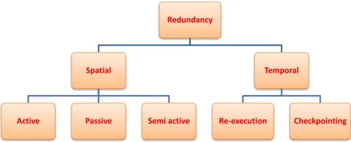
3.3.3. Redundancy for fault tolerance
As defined by [Zammali 2016], fault tolerance aims to avoid failures despite the faults present, and is essentially based on redundancy. Redundancy is when you create multiple copies of a component (hardware, software, data, etc.) or run so that the copy performs the same function, service, or role as the original component (or execution).
28
According to [Dubrova 2013, Motaghi and Zarandi 2014, Zhang and Chakrabarty 2006, Izosim et al, 2008] two families of redundancy are used in fault tolerant real-time systems (Figure 3-5): the family of spatial redundancy and the family of temporal redundancy
(time-based redundancy).
Figure 3-5 Different types of redundancy in real-time systems
3.3.3.1. Time-based redundancy methods:
In time-redundancy method additional time is spent to recompute a failed computation on the same hardware. This scheme works well for the transient faults as they are not likely to repeat during recomputation [Nikolov 2015].
RE-EXECUTION
The simplest fault tolerance technique to recover from fault occurrences is re-execution [Izosim 2009]. With re-execution, a task is executed again if affected by faults. The time needed for the detection of faults is accounted for by error detection overhead. When a task is re-executed after a fault has been detected, the system restores all initial inputs of that task. The task re-execution operation requires some time for this, which is captured by the recovery overhead. In order to be restored, the initial inputs to a task have to be stored before the process is executed for first time.
ROLLBACK RECOVERY WITH CHECKPOINTING
The time needed for re-execution can be reduced with more complex fault tolerance techniques such as rollback recovery with checkpointing [Izosim et al. 2008]. The main
Redundancy
Spatial
Active Passive Semi active
Temporal
![Figure 2-3 Different states of a real-time task [Qamhieh 2015]](https://thumb-eu.123doks.com/thumbv2/123doknet/14896520.651836/23.892.292.623.700.933/figure-different-states-real-time-task-qamhieh.webp)
![Figure 3-3 Fault classes [Avizienis et al. 2004]](https://thumb-eu.123doks.com/thumbv2/123doknet/14896520.651836/37.892.72.800.142.954/figure-fault-classes-avizienis-al.webp)