Robotica (2011) volume 29, pp. 137–152. © Cambridge University Press 2011 doi:10.1017/S0263574710000780
A stochastic self-replicating robot capable of hierarchical
assembly
Georgios Kaloutsakis
∗
and Gregory S. Chirikjian
†
∗Medotics AG, Saint-Louis-Str. 31, c/o Alltax AG, 4056 Basel, Switzerland
† Department of Mechanical Engineering, The Johns Hopkins University, 3400 N. Charles, 223 Latrobe Hall, Baltimore, MD 21218, USA
(Received in Final Form: November 11, 2010)
SUMMARY
This paper presents the development of a self-replicating mobile robot that functions by undergoing stochastic motions. The robot functions hierarchically. There are three stages in this hierarchy: (1) An initial pool of feed modules/parts together with one functional basic robot; (2) a collection of basic robots that are spontaneously formed out of these parts as a result of a chain reaction induced by stochastic motion of the initial seed robot at stage 1; (3) complex formations of joined basic robots from stage 2. In the first part of this paper we demonstrate basic stochastic self-replication in unstructured environments. A single functional robot moves around at random in a sea of stock modules and catalyzes the conversion of these modules into replicas. In the second part of the paper, the robots are upgraded with a layer that enables mechanical connections between robots. The replicas can then connect to each other and aggregate. Finally, self-reconfigurability is presented for two robotic aggregations.
KEYWORDS: Swarm robotics; Robotic self-replication; Modular robots; Mechatronic systems; Manufacturing; Mobile robots; Multi-robot systems; Robotic self-diagnosis; Self-repair.
1. Introduction
1.1. Self-replicating machines
Self-replicating machines are man-made systems that can demonstrate reproduction. Such systems can be robots, computer algorithms, biochemical processes etc.34 The concept of self-replicating machines was introduced by John von Neummann, who worked on the logic behind self-replication.25In the past there have been many other works on machines building machines. Such a reference is Paley’s teleological argument,28which was more on the philosophy of self-replication than on applied science. Other than that, Paley also discussed if a replica should be considered as a product of the replicator or of the designer of the initial seed. Self-replication together with evolution can be considered as nature’s vital processes. These are essential for the continuation of life. Evolution is the genetic change of populations and species in order to adapt to the changes
* Corresponding author. E-mail: [email protected]
of the environment. Self-replication maintains the existence of species by multiplying the number of individuals in a population. We will demonstrate self-replication with elements of evolution with a robot that can assemble into complex formations.
1.2. Self-replicating robots
Over the last several decades scientists have tried to imitate biological reproduction.14, 25, 29, 30 Space exploration and development is the most often used motivating application of self-replicating robotics.33In such a scenario, self-replication from in-situ resources is a way to maximize impact for minimal launch payloads. This concept was studied by Freitas et al. in the early 1980s, and is reviewed in ref. [10]. Chirikjian et al.7 developed a framework for mobile
self-replicating robots for Lunar development. In the same direction Suthakorn et al.37demonstrated a self-replicating
robot in a structured environment. In that work, a replicator followed lines and then picked up distinct sub-parts and placed them in known places. The parts were brought one after another by the robot to an assembly area. There, the replica was assembled until it was made fully functional. After that, the replicator was manually disassembled into its parts and the initial replica started playing the role of the replicator demonstrating the ability of manufacturing identical copies of itself. Those authors presented similar machines that were controlled by humans, which had the manufacturing capabilities of reproducing themselves.37, 38
Zykov and Lipson developed a serial robotic manipulator composed of modules that was able to self-replicate by assembling modules.47, 48 A serial robot of four identical
modules was placed onto a table. The first module was fixed on the table and the robot could move as a vertical snake. Spare modules were placed on a pallet on the table and the robot would assemble them into a new robot that had the shape and the functionality of the replicator. The environment was fully structured (the parts were placed by the authors to specific places), the replicator was controlled externally by a computer and the modules were added onto the table during the process. In the case of ref. [47], the self-replicating robot should be considered as the set of modular structures together with the computer controlling them and not only the mechanical structures. Yim,42 Murata,23 and Yoshida44
demonstrated modular structures that could demonstrate similar behavior. We will later discuss the difference between modular self-assembly and self-replication.
The need for demonstrating self-replication in more com-plex environments was motivated by Lee and Chirikjian.18 They developed a robot that was able to self-replicate in semi-structured environments. In that work, a robot controlled by a low-complexity electrical circuit moved freely in a plane until reaching painted lines that it subsequently followed to find parts. The parts were then assembled into a replica. The pieces were randomly placed onto tracks with a barcode indicating each part. The replica was assembled by connecting the parts with a specific order. By reading a barcode, the robot could determine if the part was the next one that should be added. The environment was semi-structured because the parts were not set up in a specific order.
The topic of the degree of complexity of a self-replicating robot was introduced by Lee et al.19 They developed an
entropy-based method for measuring the degree of self-replication. The approach was based on the number of parts that compose a replica, as well as the number of elements in a part. Motivated by that, Adams and Lipson1 developed another entropy-based approach for measuring the self-replicability of systems. Their model can be applied to self-replicating systems that evolve as well. Their idea is that self-replication is not a binary operation, but in nature it is combined with the evolution of replicas.
Another interesting approach on the topic are the self-replicating prototypers.20 These are machines that are able
to manufacture the components from which these are constructed. These include Bowyer’s RepRap machine2
and Matthew Moses Universal Replicator.10 Moses et al.22
recently presented a new cyclic fabrication system (CFS) that can manufacture the majority of its constituent components. On the basis of modular components, a self-replicating system produces the components that can be assembled into a replica. An example of a system’s component is a DC brush motor that can be manufactured by the CFS and is also used to operate it. Until now, self-replicating robots that have been presented were not able to perform tasks other than assembling themselves from parts. On the other hand, no robot would be developed for real-life applications without the ability to perform a useful task. Therefore, this paper addresses the design and implementation of robots that not only self-replicate but also cooperate to form larger struc-tures, which at some level is similar to the work presented by Dorigo et al.,8though the details are very different. 1.3. Self-assembly versus self-replication
replication is often confused with self-assembly. Self-assembly refers to systems that form organized structures from components in the absence of an initial replicator.41
These components are usually modules identical to each other. Self-assembly can also be viewed in two different directions: static and dynamic assembly. In static self-assembly the system reaches an equilibrium point, while in dynamic self-assembly the system can reach different form-ation states. Griffith et al.11 demonstrated blocks that were self-assembling into strings. Klavins et al.24 demonstrated programmable self-assembly of modules on an air table.
A self-assembly system is an independent set of sub-pieces that rearrange themselves. On the other side, a self-replicating system consists of a replicator and enough
parts/materials that can be assembled/manufactured into a replica. This system autonomously evolves to a set of a replicator and a replica. Modular robots that have demonstrated assembly are also able to demonstrate self-replication of structures. The difference between previous work and our approach is that previously either the robots were in structured environments or had centralized control combined with advanced sensing, whereas ours is completely distributed in an unstructured environment.
Self-replicating systems should first of all be autonomous. The replica must be identical to the replicator and that includes the controller and the algorithm controlling the replicator. In ref. [6], four categories of robotic replication are presented: directed replication via module assembly and via fabrication, reconfigurable modular robots and self-assembly via randomly agitated modules. As we will see, our robot falls in the first category but then gets upgraded and can demonstrate the third and the fourth case as well.
1.4. Modularity
A second biological characteristic that researchers have imitated in robotics is the modular or hierarchical nature of biological materials. In this setting, larger structures are assembled by simpler units, which are produced by basic elements.43 Modules of modular robots can be considered as simple units that assemble to larger structures. In large numbers they can assemble to almost any desired shape. These larger structures then walk, crawl, spin, manipulate items and drive through narrow spaces etc.23, 42, 44 Modular robots are a great tool because of their ability to reconfigure.3, 13, 32, 33Another application that modular robots
have performed is self-replication of structures. A modular robot forms a gripper, which in turn assembles more modules to an identical gripper.46, 48
2. Goal
In this paper, we present an approach that combines the above topics (self-replication and modular robotics) and demonstrates self-replicating modular robot that gets assembled hierarchically from basic modules. We study the statistics of a stochastic self-replicating robot in unstructured environments, with minimal control and without advanced sensing. After that, the robot gets upgraded to the point that allows connectivity between different robots through the use of docks. A high number of formations is then possible. Finally, simulation tools are used to study the number of produced different aggregations. This paper addresses the design and implementation of robots that not only self-replicate but also cooperate to form larger structures.8
3. Robot Development
3.1. Introduction
The intelligence and information-gathering ability provided to robots by microprocessors, sensors, cameras and other electronic components can be replaced in part by smart mechanical design.21 A fully self-replicating robot in the
A stochastic self-replicating robot capable of hierarchical assembly 139 future should not only assemble its parts but also manufacture
them. The simpler a self-replicating robot is the more feasible it is to manufacture its components from raw materials. In the same direction, smart design can also help the ability of replication in unstructured environments. We wanted to develop parts that will assemble under arbitrary initial conditions. Such include Penrose’s parts29, 30 that can be placed in a box and after shaking the box they can fit together. This minimizes the control needed for assembling the parts. (Note: An important difference between our work and that of Penrose is that in ours there is no external agitation; all actions are taken by the robot without the assistance of any external agent.) No grasping is needed but assembly can be guided by rearranging the parts together with the use of magnets for bonding the sub-systems to each other. A self-replicating robot designed under that principle needs no sensors for performing its reproduction.
3.2. Design
We propose the development of an autonomous mobile robot that consists of nm identical modules/parts. The replica’s
modules are randomly placed inside the environment at any position and orientation. The initial robot moves around finding modules, pushing them around and so forcing them to replicate to a new robot that starts running after the complete assembly of its nmmodules. There are two key features in
our model. First, there is only one way that the modules can get attached to each other, and second, when nm modules
get attached, they create a replica. Combining these two characteristics, we see that there is only one way that nm
modules assemble to each other.
The advantage of such a model is that we can assemble a new robot with minimal control and no sensory feedback from the environment. When trying to put two modules together, they get attached only if their relevant orientation is a specific one and they always result in the same double module. In the same way, if we want to add one more module to this set, there should be only one way that this module can get attached to it and will always result the same triple part set. This extends up to the nmth module, which assembles a
full robot that has exactly the same structure as the replicating robot.
We designed a robot that can fit the above model. The robot has the shape of a circular disk divided into nmidentical
pieces, such that each of the nm modules has a
pizza-slice-shape with (360n
m)
◦ angle. We will demonstrate the case when nm= 3. The modules are indeed equivalent and can only
be assembled in one way. The assembly is a result of the permanent magnets that are placed on the two sides of each module. The right side of a module must get attached to the left side of the next module. The magnets on these sides are placed with opposite orientation. This prevents the modules from getting attached in the wrong way, e.g. left side of a module getting connected to the left side of another module. In this way, if we deposit a number of modules in an environment and move the same around and there is a time that the right side of a module will get attracted to the left side of another module, they will get connected to each other, and will result in a double-part module. This double-part module will have a right side that can connect to the left side and a
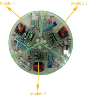
Fig. 1. Three identical modules form one robot. Each module has the following elements: batteries (1), servo motor (2), basic stamp controller (3), omnidirectional wheel (4) and permanent magnet (5).
left side that can connect to the right sides of the modules left in the environment.
Since the modules are identical, the full robot will have nm
wheels installed. We are using omnidirectional wheels that result in holonomic motion because they do not restrict the motion in any direction. A traditional type of wheel would cause a spinning type of motion. Along with each wheel, there must be a motor driving it, a control circuit driving the motor and a battery to power both the control circuit and the motor. As we have already mentioned, this is because all modules have to be identical. Since in our case, three modules assemble into a robot, each robot will have a 3-omnidirectional wheel architecture (Fig. 1).
For the control of each robot, we use a Basic Stamp 2 module by Parallax, Inc. The power of each module is off until all three modules assemble to a robot. We achieve this with the use of a conductive metal insert on both sides of each module (Fig. 3). The technique was introduced by Suthakorn
et al..38 If a module is assembled both on it’s right and
left sides, then we have at least three modules assembled with nm= 3 being the maximum number of modules; which
means a new replica has been completed. The power circuit of each module will then be closed by the metal inserts of the next module, and the robot starts running immediately after it gets assembled (Fig. 2).
This could also be made with touch sensors that would signal the controller of a full assembly. Our strategy though is to use as few sensors as possible and keep the control as simple as possible. With our approach the modules and their robot are “alive” only after a full assembly.
3.3. A self-replication scenario
Our goal was to have a robot that will self-replicate by assembling at least three parts to a replica when putting it together with those three unassembled parts in a non-structured environment. If the robot is programmed to move
Fig. 2. A single module. On the side we can see the metal inserts that are used to turn on the robot after assembly is completed.
Fig. 3. A module is ready to snap in a double module and form a robot. The magnets installed on the sides of each module are in such orientation that connectivity is possible only for producing the desired replica. Metal inserts on the side operate as power switches that turn the robot on only after the replica is fully assembled.
in a way that covers the whole area of the environment, eventually it will change the position of the modules and will continue doing so until the point where the modules will end up in a position and orientation that assembles them first to double-part modules and then to a full robot. The existence of more than three modules in the environment will make it easier for the robot to replicate its first copy. Also, if the number of modules is larger or equal to six, when the first replica gets assembled, then it will start moving around and change the position of the modules in the environment with a faster rate than the initial robot would do by itself.
Our environment is bounded and unstructured because it does not have lines, tracks or other forms of information that replicas can use for navigation. The modules to be assembled can be positioned randomly in the arena in contrast with other self-replicating robots in literature that operate in semi- or fully-structured environments.18, 47Replication can also take place with random obstacles placed in the environment, but we are going to limit our work at this point to bounded environments with no obstacles. We will later demonstrate a case with fixed obstacles in the arena. We present self-replication in a bounded environment.
In order to keep our robot’s complexity low18, 19 and
meanwhile have it moving around covering every space
of the environment, we program the robot to run with white noise frequency pulses as input to each motor. This causes Brownian type motion. The robot does not use any feedback from the environment regarding its position or the number and position of the other modules, or robots in the environment, and thus the number of elements in its control circuit remains low. The easiest way to produce the white noise pulses would be to install a radio receiver in every module and amplify its output, which in most cases is pure white noise. We preferred to use the Basic Stamp controller, which is easier to install and will give us the ability to try different kinematic strategies in the future without doing any hardware changes.
Our robot achieves self-replication through self-assembly. It is not capable of manufacturing its parts. We will later show an upgrade to the robot that sets the basis for a universal behavior. According to Suthakorn’s et al.38 categorization, our robot falls into the directed replication single-robot-without-fixture group. A single robot is able to assemble a replica without the use of external fixtures. According to Lee and Chirikjian,18 the replication process would fall into Active Replication, since for the same reason as above, a single robot can achieve assembly of replicas. Finally, according to Chirikjian,6our robot falls into Directed
Replication via module assembly.
The robot’s kinematic equations have been computed used in deriving the Fokker–Planck equations.15, 45
4. The First Experiment
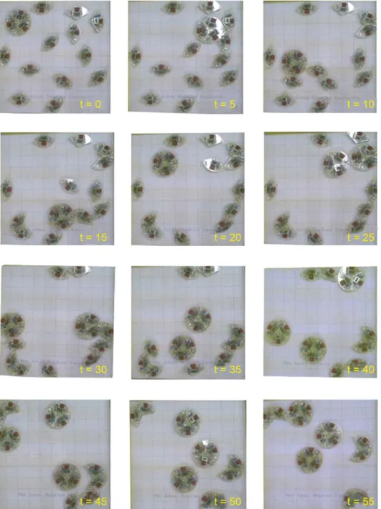
We place a robot and n= 12 unassembled modules in a one-by-one meter, planar and bounded area (Fig. 6). The motors of the modules are programmed to operate in bidirectional mode with white noise values as the magnitude of their speed. This causes the wheels to spin in random directions with random velocities that are generated from a normal distribution. Since the robot’s movement is holonomic, the robot will move randomly in every direction with the Brownian-style motion. In this way, the robot will eventually cover all points of the planar surface. We randomly place the modules to be assembled in the environment. As the assembled robot moves around, it bumps into the modules, and changes their positions. Eventually, as the positions of the modules change, some of them will come close enough to each other and get connected because of the permanent magnets.
Robots have limited energy resources. After a point, the power provided by the batteries is reduced, which results in reduced speed as well. We consider that self-replication is completed either when there are no motions in the arena, or there are no unassembled modules left. At the end of the replication process, there will be some single and double nonfunctional modules together with the operating robots of three modules. This is because, if for instance n is an even number, n modules can be assembled from n2 double modules up to n3 robots and m double modules, where
m= 1, 2. There is though a chance that the replication
will not finish due to the consumption of available energy resources.
A stochastic self-replicating robot capable of hierarchical assembly 141
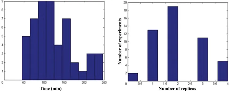
Fig. 4. (a) Histogram of the experiment durations. (b) Histogram of the number of the replicas.
There are five possible outcomes for our experiment: (1) No replica gets assembled. All single modules are
either participating in double formations or remain unassembled.
(2) One replica gets assembled. The replica works together with the replicator, and up to four double formations might been assembled.
(3) Two replicas get assembled. The replicas work together with the replicator, and up to three double formations might get assembled (Fig. 6).
(4) Three replicas get assembled. The replica works together with the replicator, and up to one double formation might get assembled.
(5) Four replicas get assembled. There are no unassembled elements left in the environment.
Performing a single run gives us no guarantee regarding the assembly of a replica. If the first scenario occurs, there will be no self-replication. We are interested in the statistics of the process. Questions like “what is the most probable outcome for our process” can be answered by studying the process over several experiments. Since at this point we are not aware of how initial conditions influence the final result, we should use the same initial conditions for all the trials.
All the trials were done under the same initial conditions. The environment used was a 100 cm× 100 cm bounded surface. Coordinates for the system’s parts were generated with the use of a random number generator. We used MATLAB to generate x, y and θ for the replicator and
the 12 modules. The numbers were generated by a uniform distribution. The pieces were placed one by one at the coordinates. If two parts end up occupying the same space for the generated coordinates, a set of new numbers was generated and the same check was performed.
4.1. Results
We recorded the times needed for finishing 50 self-replication experimental runs as well as the number of robots assembled each time. The more replicas assembled, the more successful we consider the run. The mean of the assembly time for all the modules is 124.6 minutes with the minimum time being 44.74 min. and the maximum 246.72 minutes (Fig. 4(a)). The average number of robots assembled was 2.08 (Table I). In four cases, all the modules formed robots, and in two cases six double modules were formed with no replica produced (Fig. 4(b)).
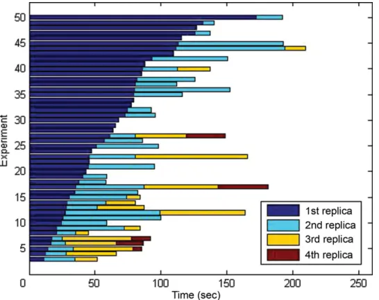
In Fig. 5, we see how the assembly events (instances where a new replica is being developed) are distributed throughout the experiment. There is no significant relationship between the duration of the events other than in cases where the first replica was assembled relatively soon; more replicas were assembled afterwards. This happened because the replica was working together with the replicator and parts were agitated at faster rates. The experiments were recorded with a static camera. We converted the video to a series of images and used Matlab’s motion detection algorithms for tracking the replicator’s movements. In this way, we managed to extract
Table I. Results of the experiments for the time events of a self-replicating process with one robot and 12 unassembled modules in the arena. For each number of replicas produced we note the standard deviation, the mean, the median, the minimum and the maximum value.
1st Replica 2nd Replica 3rd Replica 4th Replica End
St. Dev. 37.55 46.80 47.26 43.78 51.76
Mean 62.61 92.47 103.67 118.73 124.60
Median 59.1 87 84.13 92.10 114.02
Min. 11.40 25.2 44.74 85.12 44.74
Fig. 5. Bar-graph for the development of new replicas vs. time in seconds during 50 experiments. For each experiment, we note the time instance for the first replica to be assembled and then the instance for the rest of the replicas produced. For the experiments in which the maximum number of replicas has not been achieved, the end of bar indicates the time for the last replica to be produced.
the coordinates of the replicator during the process. Due to the large size of the data, we reduced the sampling to 10 frames per second. A total of 37,380 were analyzed. The coordinates were combined, and in Fig. 7 we can see the diffusion for the robot’s position. The robot moves almost uniformly around the environment. There is a higher probability around the initial position and the environment’s borders. When the robot reaches the end of the arena it bounces to the edge but still remains in the same area. Thus, it is logical that it will spend some time before changing direction and escaping toward other areas.
A pseudo-dynamical (Fig. 8) and a stochastic simulation (Fig. 9) were developed to study higher populations than the one tested above. The first one is based on the physics of body collisions, and the second one on the discretization of motions on a hexagonal lattice. Details regarding the results and the physics behind the simulations can be found in ref. [16].
5. The Upgraded Robot
5.1. The module
A module has been developed as an upgrade to the SRR modules described before.15 The goal was to add an extra layer to the robot without changing the functionality of the initial one (Fig. 10). We removed the upper layer, which was serving as a cover to the module and installed the upgraded part, which gives the robots the ability to connect with each other and form larger structures26(Fig. 12). This additional
part has been developed in such a way that it does not
change the ability of the robots to self replicate. All the characteristics of the initial modules remain as they are and a new characteristic of robots connecting each other is added. Our initial robot was a modular self-replicating robot, but its modules could assemble only to one functional structure, which was a replica.
The strategy we followed was to transform the robots from a circular to a hexagonal shape. Each robot in this way will be able to connect to six other robots. If all robots connect to others in a tight formation, a hexagonal lattice will be created. Robots should be able to assemble into any shape in the hexagonal lattice, e.g., robots can assemble to a “2D gripper” and demonstrate manipulation. After that the replicas can self-assemble to form other structures and perform more complicating functions. The greater the number of available robots, the higher the number of possible shapes that can be made.
We have two degrees of modularity. Our modules assemble to form robots and the robots operate as modules of another system. The unassembled modules are not assembling with replicas. The same thing happens in nature when molecules connect to form larger structures. We can compare modular robots with molecules and our modules with atoms. These atoms (modules) assemble to form molecules (robot) and the molecules assemble to form larger structures. We call this approach Hierarchical Self-Replication. The self-replicating process remains a directed-replication-via-module-assembly. In addition to that, it becomes a replicating reconfigurable modular robot and a self-replicating robot that performs self-assembly via randomly agitated modules6(Fig. 11).
A stochastic self-replicating robot capable of hierarchical assembly 143
Fig. 6. A robot and 12 modules are placed in a bounded environment. The robot will move around and produce replicas from the unassembled modules. At t = 50 min., we have two replicas and three double modules produced. After that point, the coordinates and the orientation of the parts in the arena might change, but no new formations will be assembled.
We added extra metal inserts on the sides of each module. The metal inserts, except of turning the power on when the modules are assembled to form robots, will serve as communication ports (Fig. 13). This gives the modules the ability to communicate with each other and program their function, as we’ll see later.
The parts of the upgraded module were first designed using 3D-CAD software. Then, a prototype was developed using machinable PE sheets. The prototype was tested regarding its connectivity to the initial modules and we proceeded to manufacturing the rest of the modules.
Key to the success of our modules was the electromechanical connectors, which attach them to each other.36 Due to our experience from the initial robot we
wanted to add the following characteristics to the new modules:
• Light weight (a heavy connector would slow down the robot).
• Strong magnetic power (connecting several parts together into large formations will require the connectors to overcome the forces applied to the wheels in order to keep the robots connected).
• Low electric power consumption (high power consump-tion, e.g. electromagnets, would reduce battery life). • Reliability (if some of the connectors do not perform
well all the time, then building formations would not be possible).
Fig. 7. Contour plot for the coordinates of a replicator in real experiments. We project the frequency of visits in each area. We see that places where the robot moves mostly are the arena’s borders as well as the place where it initially started. Generally we can say that the robot uniformly moves around.
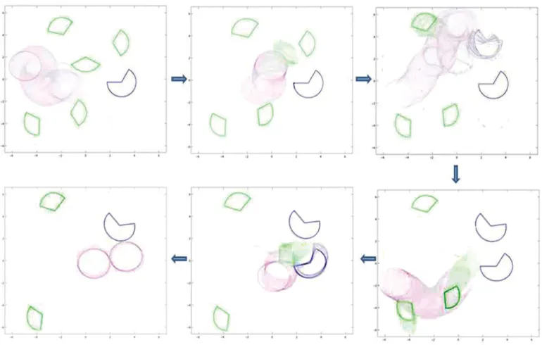
Fig. 8. An example of a pseudo-dynamical simulation with trajectories noted. A robot lies in a arena with a double and five single modules. The robot moves around and pushes two single modules to a new double module. It continues moving around and after some time pushes a single module toward a double module. A replica is being formed and starts operating.
A stochastic self-replicating robot capable of hierarchical assembly 145
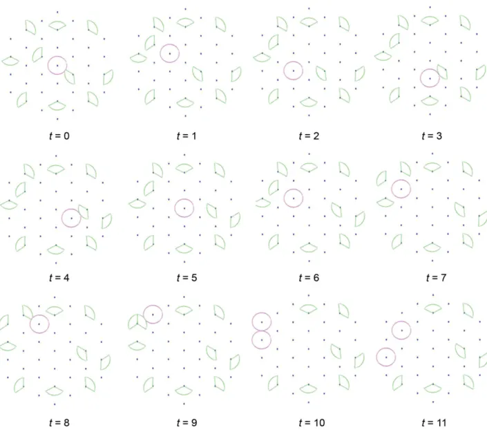
Fig. 9. Animated representation of an 11-step random walk. A robot replicates in a bounded triangular lattice with 10 single modules placed in it. The robot is represented with red, while single and double modules with green color. At t= 9 two modules are getting attached to a double formation. At t= 10 the double module is being pushed toward a single module. The orientations are such that a replica is produced. The replica starts running in the next step.
• Low manufacturing cost (as with rest of the parts that we have developed till now, the cost should remain low in order to be able to develop several pieces).
The above characteristics can be found on permanent magnets like the ones we used to connect the modules to each other. They are light weight, very strong, reliable, cheap and, finally, do not need electric power to operate. The disadvantage, though, of permanent magnets is that they always connect to each other and do not give us the ability to choose the robot sides that should be connected. In order to do this, we use a small size servo motor, which slides the base of the magnets in and out. The servo has a gear, which rolls on a track. The track is installed on the base of this new layer. If we want to set a dock available for connection, it will slide out until the connecting side with the magnets attached reaches the module’s outer part. Each module has two slides. On the top of each slide there is one dock. The docks are identical to each other. Each robot has six docks available for connection.
Fig. 10. On the right side we see the robot’s first generation, while on the left we see the alterations that took place in order to use it as a base to the upgraded robot.
The holonomic motions that were performed by our SRR robot will continue to exist even when the robots connect to larger structures. The motion of each robot will be constrained due to the connectivity but the whole group will be able to move toward any direction. We will later discuss the motions performed.
Fig. 11. Modules assemble to robots and robots form aggregations. Other than self-replication, self-assembly and self-reconfigurability can now be performed.
Fig. 12. MSRR’s extra layer. Each platform has two slides. On each slide a connector is installed. Each connector has a motor for moving on the slide and permanent magnets that allow connectivity. There are also metal inserts used for communication.
5.2. Communication
There are two different types of communication modes. The one is between the modules of the same robot and the other is between the connected robots.
Modules communicate through the metal inserts and plates, which are installed on their sides. Each robot has an input and output port on each side. The output of a module is connecting to the input of the next module and vice versa. The communication signals are bytes that represent events in a manner analogous with the bar codes used by ref. [18]. Each robot has one controller on every module but these controllers cannot operate in parallel for programming the robot’s connectivity.
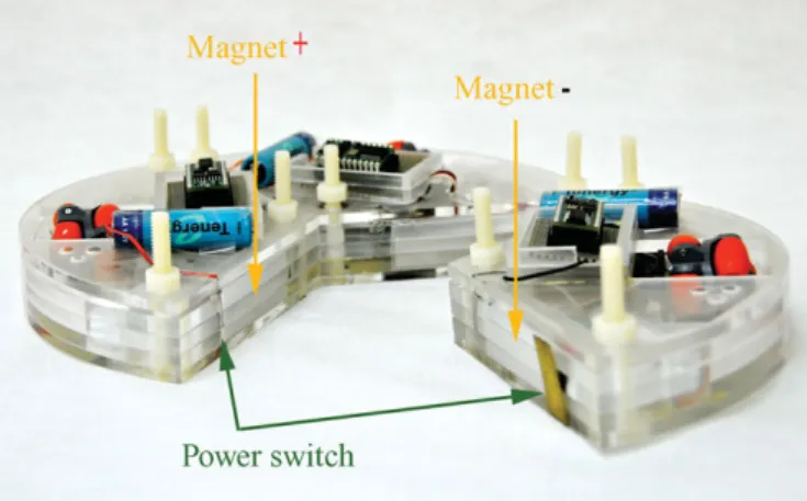
Fig. 13. A double-module formation of MSRR modules. Metal inserts on the sides are used for transferring communication tokens.
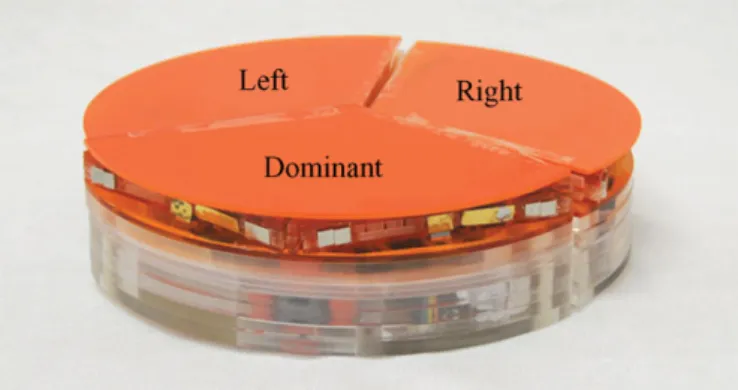
Fig. 14. A dominant module is defining the role of the rest modules in the case of programmable formations.
As the robots are mostly making random motions (except for the event of separating connected robots), programming is only needed for operating the docks and producing programmable modular formations. Out of the three modules, one module is programmed for operating the robot and the other two operate based on its directions. We will be referring to this module as dominant. Next to the dominant module, clockwise, will be the left module and the third module will be the right module (Fig. 14). Following that strategy (clockwise), the dominant module’s first dock will be enumerated as dock 1 and the right module’s last dock will be dock 6. The dominant robot will pass a signal to the other two modules, which will operate their motors. The dominant robot is also controlling its own motor.
When the modules assemble to form a robot and the power on the controllers is on, each controller generates a 16-bit random number. This random number will serve as a unique serial tag on each module. That number will be like human fingerprints. It is big enough to ensure statistically that each module will have a different serial number. Each module will pass a token to its adjacent modules. The module with the higher serial number will serve as the dominant module. After a module becomes dominant, it will assign its right and left modules. Like that, each of the docks is also assigned a number based on its module type.
A stochastic self-replicating robot capable of hierarchical assembly 147
Fig. 15. Possible configurations for MSRR. The arrows indicate which of the six docks are open for connection.
The same strategy will be followed for intra-robot communication. Each of the docks that connects the robots has metal inserts, which serve as inputs and outputs. The signal outputs of one robot will serve as inputs to the next one. If we want to program the way that aggregations grow, we will need one of the robots to serve as the dominant and control the docks of other robots. The dominant module of each robot will pass a token to its connected robots with the serial number of the modules. The robot with the larger serial number will dominate the other robot. The robot will pass the dominating serial number to its next robot and in this way, in the end, the largest serial number will determine the robot that will control the aggregation.
The chance that two robots will generate the same number is 1/65, 535. That number is very small compared to the 12 modules that we have manufactured or the few modules we will use in simulations. Since the controller cannot generate a larger number than a 16-bit number, a way to decrease the chances of two modules having the same “DNA” would be to generate two numbers. If the first one happens to be equal, then the modules could compare the 2nd token. The probability of the first and the second numbers being equal is 1/4, 294, 836, 225.
5.3. Detaching
Our modules are not equipped with motors, electromechan-ical coils or electromagnets assigned for detaching pieces. In case a formation is to be separated in two parts, a connection has to be terminated. Terminating of connections takes place by moving the two parts in inverse directions. A simple strategy for doing this is pausing the operation of the connected module and moving the motors of the other two modules. In this way each of the two robots will move in opposite directions and the forces generated on the wheels will overcome the magnetic forces that keep the parts connected (Fig. 16). In case of more robots on each side, the
Fig. 16. Two robots getting attached to each other and then detach by moving in different directions.
robots that want to detach will transfer the direction of motion to the rest of the robots that participate in the configuration in order to move toward the same direction.
6. Possible Formations
Let n be the number of robots in the environment.35 We want to determine how many possible formations pncan be
performed by the robots.24We will study the case where all
n robots are connected in the formation, since all other cases,
e.g. one formation of n− 2 and another of 2 robots, can fit the general case of n robots. Out aggregations can be considered hexagonal polyominoes.
A polyomino, or else lattice animal, is a formation made by squares in a Cartesian lattice. The aggregations made at a domino game can be considered as polyominoes. Polyominoes have discreet states. They can be rotated or flipped depending on what type of problem we are studying. In our case rotation is possible, but flipping is not. Moreover, our robots will not have discreet orientations, since we are only interested in the shape of the aggregation and that can be made in many ways because our robots have symmetric sides (free polyominoes). There is no known formula giving the number of distinct polyominoes for a given number of squares.31 Algorithms have been made through counting
these distinct cases.
Our robots form hexagonal polyominoes on the honeycomb lattice. Algorithms for computing the discreet number pnof hexagonal animal lattices have been developed
by refs. [9, 12, 39 and 40]. Due to the complexity of the problem, the algorithms have been tested for n≤ 35. We will use the algorithm results for totally free hexagons and then remove the cases of reflection. The number of reflections differs for each n. We compute cases of up to 15 robots (Table II). The problem is equivalent to the number of connected clusters on the triangle lattice.39
We see that a relatively small population of robots can create millions of different formations. Programming larger populations is not possible at that point because it is hard to compute populations of more than 36 robots. In any case, some basic formations, inspired by geometrical shapes or biological processes, can be discreetly programmed for larger robot populations. Such special cases will be geometric
Table II. Number of totaly free, fixed and free under rotation pn
hexagonal polyominoes.
n Total free Fixed pn
1 1 1 1 2 1 3 1 3 3 11 2 4 7 44 9 5 22 186 34 6 81 813 143 7 331 36,401 614 8 1435 16,590 2800 9 6505 76,663 12,814 10 30,086 358,195 59,869 11 141,229 1,688,784 281,641 12 669,584 8,022,273 1,337,853 13 3,198,256 38,351,973 1,337,853 14 15,367,577 184,353,219 30,729,401 15 74,207,910 890,371,070 148,399,324
symmetries, which can occur if robots connect with a specific pattern since the number of robots will not change the way they open and close their connectors.
6.1. Random formations
The first step in testing our robots was to let them connect in random formations. Our Modular Self-Reconfigurable Robots (MSRR) have no sensors that can be used for controlling locomotion. All the motions performed are based in open loop control. Our goal is to keep motions random so that the self-replication and the modularization processes can take place in unstructured environments. That is the continuance of the self-replicating experiment, where robots were moving around randomly.
The robots after getting assembled are turning on or keeping off their electromechanical switches randomly and then move around. Since not all of the switches will be turned on, hexagonal lattices will not be always formed. Random formations are also developed while robots have all their docks open for connection (Fig. 18). In that case we expect the aggregation to grow on higher rates, as more points will be available for connection.
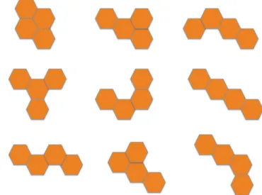
We upgraded four of the five SRRs to MSRRs. Each robot can produce 14 different combinations of connectivity (Fig. 15). We developed a grammar for describing these states. The first letter indicates how many of the docks are open to connectivity, and the letter following indicates the precise combination. Robots with zero, one, five and six of the docks open are noted with a single letter because there is only one of them with the exact number of open docks. In all four robots can produce nine different formations (Fig. 17). All of the formations with n > 4 can be reproduced by modules in one of those nine formations plus a formation for n < 4. That means, the statistical behavior of a small number of robots can be used to study systems with a higher number of robots.
6.2. Semi-random formation
We call formations that can be produced by the robots performing a unique docking combination as semi-random.27
Fig. 17. Four robots can produce nine different formations.
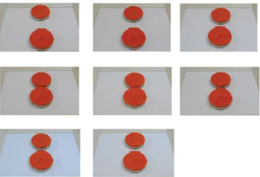
Fig. 18. A robot self-replicates. Three replicas are produced. The replicas and the replicator form a random structure with all docks open for connection.16, 17
This does not require any control, since the docks that become available for connection are programmed in their generic code.
The simplest case is when each robot operates any (out of the three) combination of symmetric docks. That function will result in linear formations for the robots. As we have seen, the robots can form aggregations on the triangular lattice. Inside the triangular lattice we can produce formations. Another example is the configuration
T-4. Robots with that configuration will form parts of a 2D
diamond lattice.
To make the above scenario possible, each of the robots should operate its docks autonomously after assembly. This happens by the dominant rule. When the robot starts operating and before it starts moving, the dominant module will indicate the robot’s docks that should be turned on. The reason why we separate these special cases from the random formations mentioned before, is that we know in advance the outcome of the self-replication despite the fact that the robots perform random motions.
A stochastic self-replicating robot capable of hierarchical assembly 149
Fig. 19. Four robots have been programmed to perform configuration T-4. The resulting formation will always be a line. Robots do not communicate with each other.
In Fig. 19 four replicas with each having two symmetric open docks (dock 1 and dock 4) are moving in a bounded test bed. When two robots come close to each other, their magnets interact. They connect through their docks and form a double robot. The double robot has two points available for connection. After some time, the third robot gets connected to an open connection. The triple robot aggregation has again two points for connection. We can see that the robots are in line. The last robot gets connected to an open connection and a quadruple linear aggregation is assembled.
This technique can be used in different cases where we want to produce complex shapes by controlling the number of parts in the assembly area. Feeding a system for some time with D-3-configured robots and then with S-configured robots will result in the formation of bars with double balls. Not all of them will have exactly the same shape or size but statistically we expect the deviation from the desired shape not to be high.
6.3. Programmable formations
Through the intra-robot communication we can achieve the development of specific formations. The system remains autonomous since it is controlled by the dominant robot’s dominant module. No external communication is established with the robots and there is no centralized computer control.
Our algorithm operates on the following steps:
• Each robot opens all of its docks, which must be connected based on its programmed formation.
• When two robots connect, they achieve the formation indicated by the dominant module.
• When a third robot connects, the system’s dominant module programs the rest of the modules. The dominant module will not change at this point. Even if the new robot has a higher serial number, it will not dominate the system. It has already been connected to one of the desired spots and will continue serving as a piece of formation that the dominant robot has already programmed. If two formations get attached to each other, detaching will be performed.
Fig. 20. A replicator produces three replicas. The replicas communicate after being connected. A “star”-shape formation is achieved.
• The last step is repeated for every extra robot attaching onto the aggregation.
• The last robot connects to the last available dock. • Last robot closes any open docks.
In order for the above algorithm to work, each module must have a specific formation preprogrammed in its control system. If all modules have been preprogrammed with the same formation, then no other formation will be reproduced. When two formations get connected, the dominant rule applies. The module that is dominating each formation will pass a token to the other formation. The aggregation with the higher token will dominate the system and control the assembly process. If needed, the dominated formation will break down into smaller pieces and remove robots not needed for assembly.
We conducted an experiment in which a preprogrammed formation number is achieved (Fig. 20). All of the modules have been programmed to produce the same formation in case they dominate the system. After a robot is assembled, each of the docks opens in order to speed up the process. After the first two robots are assembled, the dominant robot is controlling the system. It assigns the connected dock as number 1 and closes docks 2, 4 and 6. The dominated robot receives a signal to close all open modules except the connected one. The third robot randomly connects on dock 3 and receives a signal to close all of its open docks. Finally, the fourth robot connects to dock 5 and closes all of its open docks as well.
7. Self-Replication Assembly with Obstacles
The existence of random obstacles does not restrict replicas’ development. We have not studied how obstacles influence
Fig. 21. Self-replication in an environment with obstacles. A replicator navigates through obstacles and assembles two replicas, which then connect to a higher structure.
the time needed for self-replication or the replicas produced, but self-replication continues occurring. Self-replication of MSRR and hierarchically self-assembly of the replicas will continue happening with obstacles in the environment. In Fig. 21 we place a robot and nine unassembled modules in a bounded area. Two fixed obstacles are placed in the middle of the test bed, virtually separating the arena into two parts. The obstacles are close to each other. A robot can navigate from one part of the arena to the other only by moving through two obstacles.
Unassembled modules are placed on one side of the arena and the robot on the other. The robot moves through the obstacles and reaches the area of the unassembled modules. The robot is assembling a replica. The replica is replicating a third robot. The replicas are programmed to open two symmetric docks as we did in Fig. 19. A linear formation of two robots is assembled. The aggregation continues moving in the environment looking for more robots that will allow it to grow.
We expect that moving obstacles will not block the self-replicating process either. Moving obstacles can be considered parts that change their position but are not a part of the self-replicating group. That can happen either if they move independently or they move after colliding with robots in motion.
8. Self-Reconfigurability
We believe that modularity combined with self-reconfigurability is the path toward
directed-replication-Fig. 22. Four robots demonstrate self-reconfigurability. Two double module formations are assembled. The two formations connect to each other to form a quadruple formation. Finally, the quadruple formation is reconfigured to a triple one.
via-module-fabrication.6 Our self-replicating robot was
upgraded in order to demonstrate assembly and self-reconfigurability.
Self-reconfigurability takes place by detaching parts and rearranging them. In Fig. 22 we demonstrate how a quadruple robot aggregation reconfigures to form a triple robot aggregation. The robots are aligned in order to speed up the process. Soon enough, two double aggregations are formed. One aggregation opens two more docks in order to develop a star shape. The other aggregation is opening a dock to create a “divider” shape. When the two aggregations move close enough, they are attached through the single dock opened for the second aggregation with one of the two docks opened by the first aggregation.
The first aggregation is dominating the second one and a star-like shape will be formed. The module, which was connected to the dominant aggregation, opens one more dock in order to connect, completing the necessary connectivity in that way. The second step to the reconfiguration is detaching the fourth robot, which should not be a part of the formation. This step takes place by moving the robot and the triple robot formation toward opposite directions. The robot detaches and the completion of the desired animal is accomplished.
Working similarly, we can switch from one shape to another. There is no limitation on the maximum number of reconfigurations for each robot. It can participate in such processes as long as its energy capacity allows to do so.
9. Conclusions
We have demonstrated hierarchical self-replication in an unstructured environment for the case when an individual robot consists of three parts/subsystems, and the replicated
A stochastic self-replicating robot capable of hierarchical assembly 151 robots then aggregate to form clusters composed of four
robots. By scaling our subsystems into a larger number of smaller parts (n > 3) we expect that self-replication will follow the same rules. The randomness that governs our system can be statistically manipulated by choosing different initial conditions. Self-replication is not guaranteed if our robots have limited energy resources, as would apply in real cases, but with the tools we demonstrated, we can determine setups that have high probabilities for successful self-replication.
The ability of our robots to connect to each other allows them to form aggregations. These formations can be randomly developed or preprogrammed. The preprogrammed formations can be demonstrated by semi-random control systems, where each robot is independent from others, or to an autonomously programmable system, where the system chooses a dominating robot, which programs the rest of the robots after attachment. A large number of modules will generally produce a large number of robots that can then form complex shapes.
10. Future Work
Our robots have demonstrated the ability of detaching from each other after getting connected. That, together with the modularity, can give to our robots the ability to demonstrate a series of different shapes. Reconfigurability will allow our self-replicating robot to perform a number of new functions as in ref. [3]. Such a function can be self-repair5by replacing
faulty robots with new ones picked from the environment. Fitting large aggregations through narrow spaces can also be performed through reconfigurability. The aggregation can be broken down to smaller formations, allowing them to navigate through narrow spaces and then reassemble to its initial shape as in ref [4].
Acknowledgments
This work was supported in part by NSF grant IIS-0915542, RI: Small Robotic Inspection, Diagnosis, and Repair.
References
1. B. Adams and H. Lipson, “A universal framework for analysis of self-replication phenomena,” Entropy 11, 295–325 (2009). 2. A. Bowyer, “The Self-Replicating Rapid
Prototyper-Manufacturing for the Masses,” Proceedings of the Center for
Rapid Design and Manufacture, High Wycombe, UK (Jun.
2007).
3. Z. Butler, S. Murata and D. Rus, “Distributed Replication Al-gorithm for Self-Reconfiguring Modular Robots,” Proceedings
of DARS’02, Fukuoka, Japan (Jun. 2002) pp. 25–27.
4. Z. Butler and D. Rus, “Distributed Locomotion Algorithms for Self-Reconfigurable Robots Operating on Rough Terrain,”
Proc Comput. Intell. Robot. Autom. 2(16–20), 880–885 (Jul.
2003)
5. G. S. Chirikjian, “Robotic Self-Replication, Self-Diagnosis, and Self-Repair: Probabilistic Considerations,” DARS’08,
Proceedings of Distributed and Autonomous Robotic Systems,
Tsukuba, Japan (2008) pp. 273–281.
6. G. S. Chirikjian, “Parts Entropy, Symmetry, and the Difficulty of Self-Replication,” Proceedings of ASME Dynamic Systems
and Control Conference, Ann Arbor, MI (Oct. 20–22,
2008) pp. 1301–1307.
7. G. S. Chirikjian, Y. Zhou and J. Suthakorn, “Self-replicating robots for lunar development,” IEEE/ASME Trans.
Mechatronics 7(4), 462–472 (Dec. 2002).
8. R. Gross, E. Tuci, M. Dorigo, M. Bonani and F. Mondada, “Object Transport by Modular Robots that Self-Assemble,” In:
IEEE International Conference on Robotics and Automation – ICRA 2006 (IEEE Computer Society Press, Los Alamitos, CA,
2006) pp. 2558–2564.
9. I. G. Enting and A. J. Gutman, “Polygons on the honeycomb lattice,” J. Phys. A: Math. Gen. 22, 1371–1384 (1989). 10. R. A. Freitas and R. C. Merkle, Kinematic Self-replicating
Machine (Lands Bioscience, Georgetown, TX, 2004).
11. S. Griffith, D. Goldwater and J. M. Jacobson, “Self-replication from random parts,” Nature 437, 636 (2005).
12. A. J. Guttmann and I. G. Enting,“The number of convex polygons on the square and honeycomb lattices,” University
of Melbourne, Department of Math. 21(8), 467–474 (1987).
13. R. F. Hodson, K. Somervill, J. Williams, N. Bergman and R. Jones, “An architecture for reconfigurable computing in space,”
Mil. Aerosp. Program. Log. Devices (2005).
14. H. Jacobson, “On models of reproduction,” Am. Sci. 46, 255– 284 (1958).
15. G. Kaloutsakis and G. S. Chirikjian, “Self-replicating Robot in an Unstructured Environment,” Proceedings of Romansy’08, Tokyo, Japan (Jul. 2008).
16. G. Kaloutsakis, Hierarchical Self-Replication, PhD
Dis-sertation (Baltimore, MD: Johns Hopkins University, Jul.
2010).
17. G. Kaloutsakis, Online video clip: http://custer.lcsr.jhu.
edu/Georgios, 2010.
18. K. Lee and G. S. Chirikjian, “Robotic self-replication from low complexity parts,” IEEE Robot. Autom. Mag. 14(4), 34–43 (2007).
19. K. Lee, M. Moses and G. S. Chirikjian, “Robotic self-replication in structured environments: physical demonstra-tions and complexity measures,” Int. J. Robot. Res. 27(3–4), 387–401 (2008).
20. H. Lipson, “Homemade: The Future of Functional Rapid Prototyping,” IEEE Spectr. (May 2005) 42(5), pp. 24–31. 21. M. A. Erdmann and M. T. Mason, “An Exploration of
Sensorless Manipulation,” IEEE J. Robot. Autom. 4(4), 369– 379 (Aug. 1988).
22. M. Moses, H. Yamaguchi and G. Chirikjian, “Towards Cyclic Fabrication Systems for Modular Robotics and Rapid Manufacturing,” Proceedings of Robotics: Science and
Systems, Seattle, Washington, USA (Jun. 2009).
23. S. Murata, H. Kurokawa and S. Kokaji, “Self-Assembling Machine,” Proceedings of IEEE ICRA’94, San Diego, CA, USA (1994) pp. 441–448.
24. N. Napp, S. Burden and E. Klavins, “The Statistical Dynamics of Programmed Self-assembly,” Proceedings of ICRA 2006 (2006) pp 1469–1476.
25. J. von Neuman and A. W. Burks, Theory of Self-Reproducing
Automata (University of Illinois Press, Illinois, 1962).
26. R. O’Grady, A. Christensen and M. Dorigo, “SWARMORPH: Multi-robot morphogenesis using directional self-assembly,”
IEEE Trans. Robot. 25(3), 738–743 (Jun. 2009).
27. E. H. Ostergaard, K. Kassow, R. Beck and H. H. Lund, “Design of the ATRON lattice-based self-reconfigurable robot,” Auton.
Robots 21(2), 165–183 (2006).
28. W. Paley, “Natural Theology: Or, Evidences of the Existence and Attributes of the Deity,” In: 12th edition London: Printed
for J. Faulder (1809) pp. 1–16, Published by J. Vincent,
Oxford.
29. L. S. Penrose, “Machines of self-reproduction,” Ann. Hum.
Genet. 23, 59–72 (1958).
30. L. S. Penrose, “Self-reproducing machines,” Sci. Am. 200(6), 105–114 (1959).
31. D. H. Redelmeier, “Counting polyominoes: Yet another attack,” Discrete Math. 36(2), 191–203 (1981).
32. W. Shen, Y. Lu and P. Will, “Hormone-Based Control for Self-Reconfigurable Robots,” Proceedings of International
Conference Autonomous Agents, Barcelona, Spain (2000)
pp. 1–8.
33. W. Shen, P. Will and B. Khoshnevis, “Self-Assembly in Space Via Self-Reconfigurable Robots,” Proceedings of IEEE, Taipei, Taiwan ICRA’03, (2003) pp. 2516–2621.
34. M. Sipper, “Fifty years of research on self-replication: An overview,” Artif. Life 4(3), 237–257 (1998).
35. A. Skliros and G. S. Chirikjian, “Position and orientation distributions for locally self-avoiding walks in the presence of obstacles,” Polymer 49(6), 1701–1715 (Mar 17, 2008). 36. K. Stoy, D. J. Christensen, D. Brandt, M. Bordignon and U. P.
Schultz, “Exploit Morphology to Simplify Docking of Self-Reconfigurable Robots,” Proceedings of DARS’08, Ibaraki, Japan (2008).
37. J. Suthakorn, A. B. Cushing and G. S. Chirikjian, “An Autonomous Self-Replicating Robotic System,” Proceedings
of IEEE International Conference on Advanced Intelligent Mechatronics, AIM’03 (2003) pp. 137–142.
38. J. Suthakorn, Y. Kwon and G. S. Chirikjian, “A Semi-Autonomous Replicating Robotic System,” Proceedings of
2003 IEEE CIRA, Kobe, Japan (Jul. 2003).
39. M. Vge and A. J. Guttmann, “On the number of hexagonal polyominoes,” Theor. Comput. Sci. 307(2), 433–453 (2003). 40. M. Voge, A. J. Guttmann and I. Jensen, “On the number of
benzenoid hydrocarbons,” J. Chem. Inf. Comput. Sci. 42(3), 456–466 (2002).
41. P. J. White, K. Kopanski and H. Lipson, “Stochastic self-reconfigurable cellular robotics,” Proc. ICRA 2004 3(26), 2888–2893 (2004).
42. M. Yim, D. Duff and K. Rufas, “PolyBot: A Modular Reconfig-urable Robot,” Proceedings IEEE ICRA02’, Washington, DC, USA (2000) pp. 514–520.
43. M. Yim, W. M. Shen, B. Salemi, D. Rus, M. Moll, H. Lipson, E. Klavins and G.S. Chirikjian, “Modular self-reconfigurable robot systems – challenges and opportunities for the future,”
IEEE Robot. Autom. Mag. 14(1), 43–52 (Mar. 2007).
44. E. Yoshida, S. Murata, A. Kamimura, K. Tomita, H. Kurokawa and S. Kokaji, “A self-reconfigurable modular robot: Reconfiguration planning and experiments,” Int. J. Robot. Res.
21(10), 903–916 (2003).
45. Y. Zhou and G. S. Chirikjian, “Probabilistic models of dead-reckoning error in nonholonomic mobile robots,” Proc. IEEE
ICRA 2, 1594–1599 (2003).
46. V. Zykov and H. Lipson, “Fluidic Stochastic Modular Robotics: Revisiting the System Design,” Proceedings Robotics: Science
and Systems Workshop on Self-Reconfigurable Modular Robots, Philadelphia, Pennsylvania, USA (Aug. 2006).
47. V. Zykov, E. Mytilinaios, B. Adams and H. Lipson, “Self-reproducing machines,” Nature 435(7038), 163–164 (2005). 48. V. Zykov, E. Mytilinaios, M. Desnoyer and H. Lipson,
“Evolved and designed self-reproducing modular robotics,”