Fluidmechanics of semicircular canals - revisited

0044-2275/08/030475-23 DOI 10.1007/s00033-007-6037-7

c

° 2007 Birkh¨auser Verlag, Basel

Zeitschrift f¨ur angewandte Mathematik und Physik ZAMP

Fluidmechanics of semicircular canals – revisited

Abstract. In this work we find the exact solution for the flow field in a semicircular canal which is the main sensor for angular motion in the human body. When the head is rotated the inertia of the fluid in the semicircular canal leads to a deflection of sensory hair cells which are part of a gelatinous structure called cupula. A modal expansion of the governing equation shows that the semicircular organ can be understood as a dynamic system governed by duct modes and a single cupular mode. We use this result to derive an explicit expression for the displacement of the cupula as a function of the angular motion of the head. This result shows in a mathematically and physically clean way that the semicircular canal is a transducer for angular velocity. Mathematics Subject Classification (2000). 76Z05, 74F10.

Keywords. Semicircular canal, biofluiddynamics, modal expansion, adjoint eigenvalue problem.

1. Introduction

The vestibular organ (Figure 1) located in the inner ear of humans and numerous animals is the primary sensor for angular and linear motion. The semicircular canals are part of the vestibular organ. They are specifically responsible for sensing rotations. In each ear there are three semicircular canals which are oriented in mutually orthogonal directions. The canals are carved in bone and are filled with perilymph and endolymph, two fluids with mechanical properties similar to water. The endolymph and the perilymph are separated by a membranous duct. At one end of each semicircular canal there is the ampulla which contains the cupula. The cupula is a gelatinous structure which fills the entire cross-section of the canal such that the flow of the endolymph is blocked [15]. All three canals connect to the utricle, a larger chamber which also contains one of the sensors for linear motion. Under angular motion the inertia of the endolymph in the semicircular canals leads to a deflection of the cupula. This activates sensory hair cells in the cupula which send an electrical signal to the central nerve system. For the purpose of our present investigation it is sufficient to assume that the sensation of angular motion is roughly proportional to the deflection of the cupula. The relationship between mechanical effects and afferent nerve discharge in the cupula is discussed in detail

cochlea

@ @

@ @

anterior semicircular canal

B B

B BB

posterior semicircular canal

££ £££

lateral semicircular canal

´´ ´´ ´´ vestibule B B BB

Figure 1. The human vestibular organ

in [28] and [12].

Clearly, the dynamics of the fluid flow in the semicircular canals is the key to the proper operation of the sensor for angular motion. Many authors have investigated this flow problem. The actual discovery of the role of the vestibular organ as the main source of sensation of motion is due to Ewald in 1892 [9]. Steinhausen [23] was the first to postulate a mathematical description for the sensation of angular motion. He modeled the dynamics of semicircular canals as a strongly damped torsional pendulum. This model describes the main features of the dynamics of the semicircular canals. The values for the parameters of this simple macroscopic model, however, remain unclear. Several authors (for instance, [21], [27]) have tried to model these parameters by assuming Poiseuille flow in the semicircular canals.

Van Buskirk & Grant [25] and later Van Buskirk, Watts and Liu [26] departed from the macroscopic Steinhausen model and derived equations for the axisymmet-ric flow in the slender part of the canals directly from the Navier–Stokes equations. Oman, Marcus & Curthoys [16] introduced a more complex description of the ge-ometry of semicircular canals but remained with a one-dimensional model for the

dynamics. Rabbitt & Damiano [17] used an accurate three-dimensional model of the canal and found an asymptotic solution for the flow field. This work was fol-lowed by Damiano & Rabbitt [7] who did a detailed analysis of the flow field in the ampulla. They used the slenderness ratio (ratio between the minor and the major radius of the torus) as their asymptotic variable ǫ. The flow field in the slender part is considered the outer solution, whereas the flow in the ampulla is considered the ’boundary layer’ or inner solution. The two solutions are asymptotically matched by balancing terms with equal powers of ǫ. They found that the flow in the slender part is barely influenced by the more complicated flow field in the ampulla. Or in other words, the dynamics of the endolymph is dominated by the viscous flow in the slender part of the canal. In retrospect, this important result is justification for the simplifications by Van Buskirk et al. [26] who only looked at the flow in the slender part of the canal for which a constant circular cross-section was assumed. Although all these investigations used different models and assumptions they all agreed with the basic dynamic features of the Steinhausen model.

In this work we will present an exact solution to the equation proposed by Van Buskirk et al. [26], hereafter referred to as VB. We will show that the solution can be written in a simple and straightforward form which will allow us to use it for the

R 2a ˙ α β γ r z utricle cupula ampulla

study of several clinical manoeuvres of the head. The result of this work provides a solid fluidmechanical fundament for research on disorders of semicircular canals. In §2 we briefly summarize the work of VB and re-derive their equation. In §3 we find the solution of the homogeneous form (without forcing) of VB’s equation. The reaction to impulsive forcing is derived in §4. We use this result in §5 to find the full solution to VB’s equation. This is followed by §6 where we use our solution to study a few simple manoeuvres of the head. Section 7 concludes this paper.

2. The model of Van Buskirk, Watts and Liu

For the purpose of this investigation we neglect the flow of the perilymph and consider only the endolymph and its surrounding membranous duct. Furthermore we limit our investigation to a single semicircular canal which is a sensible simpli-fication as long as we consider only head manoeuvres in the plane of the respective semicircular canal. With this simplification the membranous duct has the topol-ogy of a torus. The slender part of the duct spans an angle β and has a constant circular cross-section of radius a which is much smaller than the main radius R of the torus (Figure 2). The utricle spans an angle γ. The rotation angle α(t) (the actual head manoeuvre) is a function of time t.

An observer moving with the canal perceives an axial fluid motion u relative to the canal. This fluid motion obeys the Navier–Stokes equations. In the slender part of the semicircular canal the axial component of the Navier–Stokes equations takes the simple form

∂u ∂t + R ¨α = − 1 ρ ∂p ∂z + ν r ∂ ∂r µ r∂u ∂r ¶ , (1)

where we have neglected the influence of curvature since R ≫ a. In this equation ¨

α(t) is the angular acceleration, ρ is the fluid density, p is the pressure and ν is the kinematic viscosity. The variables r and z are components of a cylindrical coordinate system with the origin on the canal centerline. The axial velocity u is a function of r and t and independent of z due to continuity. Table 1 lists the values for the physical and geometric parameters that are used in this paper.

description value reference

major canal radius R 3.2 × 10−3_{m Curthoys & Oman [5]}

duct radius a 1.6 × 10−4_{m Curthoys & Oman [5]}

angle subtended by the canal β 1.4π Van Buskirk et al. [26] angle subtended by the utricle γ 0.42π Van Buskirk et al. [26]

endolymph density ρ 103_kg/m3 _{Bronzino [3]}

kinematic viscosity of the endolymph ν 10−6_m2_{/s Bronzino [3]}

cupular stiffness K 13 GPa/m3

calculated in §6.1 Table 1. Physical and geometrical parameters

In order to find an appropriate expression for the pressure gradient ∂p/∂z we differentiate (1) once with respect to z. All terms which contain u drop out since they are constant in z (the same goes for the term R ¨α). We obtain

∂2_p

∂z2 = 0. (2)

Therefore, ∂p/∂z is a constant and the pressure p(z) is a linear function of z. The pressure difference ∆p between the two ends of the slender part of the semicircular canal is

∆p = p(βR) − p(0) = βRµ ∂p_∂z ¶

. (3)

The pressure difference ∆p is caused by an external force F which exerts a pressure F/(πa2_{) to one end of the semicircular canal. This external pressure must be equal}

to the pressure difference ∆p which leads us to the following expression for the pressure gradient,

∂p ∂z =

F

πa2_βR. (4)

We model the external force F by the sum of the reactive force Fcof the deflected

cupula and the inertial force Fi of the fluid in the utricle (we assume the actual

fluid motion within the utricle to be negligible relative to the magnitude of u [24]). The reactive force Fc of the cupula is a function of time and is proportional

to the volumetric deflection of the cupula (for a detailed mechanical model of the cupula refer to [28]), Fc(t) πa2 = K 2π Z t 0 Z a 0 u(̺, τ )̺ d̺ dτ. (5)

The inertial force Fiof the fluid in the utricle is approximated by Newton’s second

law as

Fi= muR ¨α. (6)

However, most of the inertial force of the fluid in the utricle is absorbed by the walls at the end of the utricle. Only the fluid volume which directly pushes onto the fluid in the slender part of the canal is relevant to Fi. Therefore, we choose the

mass mu to be equal to the mass of the endolymph which is contained in a torus

section of length γR (arc length of the utricle) with cross-section πa2_{(cross-section}

of the slender canal),

Fi= ρπa2γR2α.¨ (7)

Using these expressions we arrive at the linear inhomogeneous equation for u(r, t) as given by VB [26] on p.92, ∂u ∂t + µ 1 + γ β ¶ R ¨α = −2πK_ρβR Z t 0 Z a 0 u̺ d̺ dτ +ν r ∂ ∂r µ r∂u ∂r ¶ . (8)

(Note that in contrast to VB we have named the angular acceleration ¨α instead of α.)

VB suggests the following non-dimensional variables: ˜ r = r a, ˜t = tν a2, u =˜ u RΩ, (9)

where Ω is a typical angular velocity of dimension [1/s]. In these variables we obtain the non-dimensional form of (8),

∂ ˜u ∂˜t + µ a2_{(1 + γ/β)} νΩ ¶ ¨ α = −ǫ Z ˜t 0 Z 1 0 ˜ u̺ d̺ dτ +1 ˜ r ∂ ∂ ˜r µ ˜ r∂ ˜u ∂ ˜r ¶ , (10)

where ǫ = 2πKa6_/ρβRν2_{≪ 1. Together with the initial condition ˜u(r, 0) = 0 and}

the boundary conditions ˜u(1, ˜t) = ∂ ˜u(0, ˜t)/∂ ˜r = 0 we have arrived at a well-posed problem for ˜u(˜r, ˜t).

VB now proceeds to an asymptotic solution of (10) making use of ǫ ≪ 1. Much in contrast to this we will show in the following sections that (10) can be solved exactly for an arbitrary forcing ¨α.

3. Homogeneous solution

We proceed by examining (10) without forcing (and for the ease of writing we drop the tilde of the non-dimensionalized variables). To this end we set α(t) = 0 and differentiate (10) once with respect to t to arrive at the equation

∂2u ∂t2 − 1 r ∂ ∂r µ r ∂ 2_u ∂r ∂t ¶ + ǫ Z 1 0 u̺ d̺ = 0. (11)

The ansatz u(r, t) = ˆu(r)e−σt _{reduces the partial integro-differential}

equa-tion (11) to an ordinary integro-differential equaequa-tion, σ2_{rˆu + σ ˆu}′ + σrˆu′′ + rǫ Z 1 0 ˆ u̺ d̺ = 0, (12) where ˆu′

≡ dˆu/dr. Together with the boundary conditions ˆu(1) = ˆu′

(0) = 0 this equation is a nonlinear eigenvalue problem for the eigenvalue σ. The solution of this eigenvalue problem yields modal solutions of the form ˆuk(r) exp(−σkt). For

eigenvalues σ = σr+ iσi with a positive real part σrthe modal solution decays in

time. Vice versa we obtain growing solutions for σr < 0. For σi 6= 0 the modal

solutions oscillate in time.

We can recast the nonlinear eigenvalue problem (12) into a linear general eigen-value problem by defining a new dependent variable v(r) = (ˆu(r), σ ˆu(r))T,

Av= σBv, (13) A=µ−ǫ r R 1 0(·)̺ d̺ 0 0 r ¶ , B=µr ∂ 2_/∂r2_{+ ∂/∂r r} r 0 ¶ .

This technique of expanding the dependent variable is often used in hydrodynamic stability, where the eigenvalue (in that case a spatial wavenumber α) can appear up to its fourth power (see, for instance, [22]). In the case of hydrodynamics the expanded variables αn_{u have no particular physical meaning. In our case,ˆ}

however, −σˆu(r) corresponds to the acceleration ∂u/∂t. Therefore (13) is nothing more than a reformulation of (11) in phase space (u, ∂u/∂t) which reduces (11) from a second order to a first order equation in t.

In the form (13) the matrices A and B are matrices of differential and integral operators, and the vector v is a vector of continuous functions. By applying an appropriate spatial discretization scheme we can approximate A and B by matrices with scalar entries and v becomes a vector of function values at discrete grid points rj. In our case, we use a compact finite difference scheme of fourth

order and equidistant grid spacing to discretize (13). The discretized eigenvalue problem can be solved numerically with a standard eigenvalue solver. Already less than 100 grid points give enough accuracy to resolve the first few eigenmodes.

We have listed the locus of the five least stable eigenvalues for different ǫ in Table 2. All eigenvalues are real and positive and therefore the physical system described by (11) is asymptotically stable and does not have any oscillating eigen-modes. ǫ = 0.01 ǫ = 0.017 ǫ = 0.05 ǫ = 0.09752 ǫ = 0.2 σ0 6.251×10−4 1.063×10−3 3.127×10−3 6.102×10−3 1.253×10−2 σ1 5.783 5.782 5.780 5.777 5.771 σ2 3.047×101 3.047×101 3.047×101 3.047×101 3.047×101 σ3 7.488×101 7.488×101 7.488×101 7.488×101 7.488×101 σ4 1.390×102 1.390×102 1.390×102 1.390×102 1.390×102 |κ0| 0.2500 0.2501 0.2501 0.2503 0.2505 |κ1| 0.2446 0.2446 0.2447 0.2448 0.2451 |κ2| 0.04643 0.04643 0.04643 0.04642 0.04642 |κ3| 0.01890 0.01890 0.01890 0.01890 0.01890 |κ4| 0.01019 0.01019 0.01019 0.01019 0.01019

Table 2. Eigenvalues σkand volume flow κk of the five least stable modes

Although convenient in use the numerical solution of (13) does not provide us with any profound insight into the true structure of the eigenvalue spectrum. It merely gives us numerical values for {σk, ˆuk(r)}. Therefore we put the numerical

solution aside for a while and proceed to solve (12) analytically.

At this point we make the important observation that the integral in (12) is proportional to the volume flow through the duct. This definite integral yields a value that is independent of r, i.e., a constant. With the definition

κ ≡ Z 1

0

ˆ

we can rewrite (12) as an inhomogeneous ordinary differential equation for ˆu, σrˆu′′

+ σ ˆu′

+ σ2rˆu = −rǫκ. (15)

The inhomogeneous solution of (15) is ˆui = −ǫκ/σ2. The homogeneous part of

(15) is a Bessel equation of order zero with the solutions J0(√σr) and Y0(√σr)

[1]. We can discard the solution Y0(√σr) because it is singular at r = 0 and does

not satisfy the boundary condition there. Thus, we get ˆ

u(r) = AJ0(√σ r) − ǫ

κ

σ2, (16)

where A is an arbitrary constant. Now we can eliminate κ by substituting ˆu in (14) by (16). This gives us following expression for κ

κ = Aζσ σ2 σ2_{+ ǫ/2}, (17) with ζσ≡ Z 1 0 J0( √ σ̺) ̺ d̺. (18)

It remains to satisfy the boundary condition ˆu(1) = 0. From (16) and (17) we get the relation

J0(√σ) =

ǫζσ

σ2_{+ ǫ/2} (19)

which determines all eigenvalues σ.

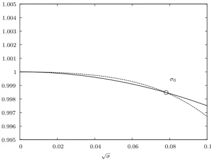
Although there is no explicit solution to (19) we can find the locus of all eigen-values by simple graphical examination. To this end we draw the graphs of the left-hand side and the right-hand side of (19) against√σ (see Figures 3 and 4). The eigenvalues σk correspond to the intersections of the two curves (marked by

circles). As expected from the numerical solution all eigenvalues are positive. The dashed curve in Figure 3, i.e., the right-hand side of (19), drops rapidly to zero, such that it intersects with the solid line in the vicinity of the first root of the Bessel function. For larger choices of ǫ the dashed curve drops more slowly. Theoretically, we can choose ǫ so large that the dashed and the solid curve do not intersect until around the second root of the Bessel function (or even later). In that case, we would loose our first few eigenvalues. However, for all physically sensible choices of ǫ the situation remains qualitatively as shown in Figure 3.

We observe that the least stable eigenvalue σ0 is very close to 0. Numerical

investigation1_{shows that σ}

0is approximately proportional to ǫ (Figure 5). We can

find an explicit expression for this relation by expanding (19) about σ = 0 (where we also assume that σ2_{≪ ǫ),}

σ + O(σ2) = ǫ

16 + ǫ/764. (20)

1 _{Even though finding eigenvalues by graphical examination is attractive and enlightening (in}

an analytical sense), we use the numerical solutions in the following since the solutions from a numerical eigenvalue solver are usually more robust and accurate (in a numerical sense) than solutions that are obtained graphically.

σ0 σ1 σ2 σ3 √ σ −0.5 0.5 1 1.5 0 0 2 4 6 8 10

Figure 3. Graphical solution of the eigenvalue relation for ǫ = 0.09752: the intersections of the left-hand side (——) and the right-hand side (– – –) of (19) correspond to the eigenvalues

σ0 √_σ 0.995 0.996 0.997 0.998 0.999 1 1.001 1.002 1.003 1.004 1.005 0 0.02 0.04 0.06 0.08 0.1

This result is consistent with the result of VB who arrived at σ0= ǫ/16 through

asymptotics for ǫ ≪ 1. All other eigenvalues σ1, σ2, . . . (there are infinitely many)

σ ǫ 0.002 0.004 0.006 0.008 0.01 0.012 0.014 0 0 0.02 0.04 0.06 0.08 0.1 0.12 0.14 0.16 0.18 0.2

Figure 5. Numerically computed least stable eigenvalues σ0 as a function of ǫ

correspond approximately to the roots of J0(√σ) since the right-hand side of (19)

is almost zero for σ > 1,

σj ≈ λ2j, j = 1, 2, . . . ,

where λj is the j-th root of the Bessel function J0. We see that there is a

funda-mental difference between the least stable eigenvalue σ0 and all other eigenvalues.

To illustrate this difference we briefly re-consider our problem for a semicircular canal without a cupula. We can eliminate the cupula from our equations by setting ǫ = 0. In that case, the right-hand side of (19) is zero. Obviously, the least stable eigenvalue σ0 is no longer a solution. The other eigenvalues, however, remain

approximately at the same locations. Apparently, these modes are independent of the presence of the cupula. They are directly related to the modes of a pipe flow. Therefore, we call them duct modes. The least stable mode exists only because of the cupula. Therefore, we call it the cupular mode.

To conclude our discussion of the eigenvalue spectrum we note that although σ = 0 satisfies (19) it is not an eigenvalue, since its corresponding eigenfunction is the trivial solution ˆu = 0.

Apart from the eigenvalues σ we can also extract the shape of the eigenfunctions ˆ

A √ σ 1 r ˆ u2(r) 0 2 4 6 8 10

Figure 6. Construction of eigenfunctions from the graphical solution of (19) on the example of the eigenfunction ˆu2(r) (note that this plot uses two different sets of axes: one with√σ on the

abscissa for plotting (19) and one with the abscissa r for the eigenfunction ˆu2(r))

Bessel functions of order zero that are shifted by a constant such that ˆu(r = 1) = 0. Therefore, we can find the shape of the j-th eigenfunction by setting the abscissa r such that r = 1 cuts the Bessel function at J0(√σj). Figure 6 demonstrates

the graphical construction of the eigenfunctions on the example of ˆu2which is the

eigenfunction associated with σ2. The higher eigenfunctions consist of increasingly

larger sections of the Bessel function.

Furthermore it is interesting to see that the eigenfunctions corresponding to σ0 and σ1 resemble the Poiseuille profile 1 − r2 (Figure 7). The similar shape of

these two eigenfunctions together with the large difference in their temporal rate of decay makes this pair of eigenmodes good candidates for transient effects [11].

This concludes our discussion of the homogeneous problem (11). We have found the complete spectrum with its corresponding eigenfunctions. In its general form the solution to (11) is u(r, t) = ∞ X k=0 Akuˆk(r)e−σkt, (21)

where the coefficients Ak are determined through the initial conditions.

We should note that the duct modes have also been found by Rabbitt & Dami-ano [17]. However, they were missing the cupular mode which they introduced only later by asymptotic matching of the flow field in the ampulla [7]. Also we

r ˆu0 (a) 0 0 0.2 0.2 0.4 0.4 0.6 0.6 0.8 0.8 1 1 r ˆu1 (b) 0 0 0.2 0.2 0.4 0.4 0.6 0.6 0.8 0.8 1 1

Figure 7. The two least stable eigenfunctions ˆu0(r) and ˆu1(r) (the dotted line is the parabolic

profile 1 − r2

)

find that the two asymptotic solutions of VB correspond to the cupular mode and the first duct mode, respectively. Whereas VB have arrived at this result through multiple-scale analysis in t and ǫt, we have reproduced their results and revealed the complete modal structure by straightforward analytical reasoning. One might argue now that the higher modes are physically irrelevant since they are so heavily damped that they cannot be observed in nature. However, we will show in the following section that the knowledge of the complete set of modal solutions is a useful asset for the computation of the inhomogeneous solution of (10).

4. Impulse response

In this section we find the solution of (10) for an impulsive acceleration ¨α = Bδ(t) of the semicircular canal. Clinically this corresponds to a sudden acceleration of the head at rest to a constant velocity ˙α = Ba2/ν (the factor a2/ν arises because the dots in ˙α and ¨α stand for the derivative with respect to the dimensional time variable).

We solve this inhomogeneous problem by recasting it into a homogeneous initial value problem. To this end we integrate (10) with respect to t from −T to +T and let T → 0. The left-hand side gives us values for u immediately before and after t = 0 as well as a constant term from the integration of δ(t). The right-hand side vanishes due to the boundedness of u, (1/r)∂u/∂r and ∂2_u/∂r2 _{(these values}

are bounded since there cannot be infinite velocities or infinite viscous forces), u(r, t = 0+) − u(r, t = 0− ) +µ a 2_{(1 + γ/β)} νΩ ¶ B = 0. (22)

Causality tells us that u(r, t = 0−

) must be 0. Therefore we obtain the initial condition u(r, t = 0+) = u0= − µ a2_{(1 + γ/β)} νΩ ¶ B. (23)

Since (10) is a second order equation in t we need a second initial condition. We obtain this second condition by differentiating (10) once with respect to t. Then we integrate this equation as before from −T to T with T → 0. In this case the forcing term on the left-hand side is zero due to the symmetry of δ(t). We obtain

∂u ∂t ¯ ¯ ¯ ¯ t=0+ − ∂u ∂t ¯ ¯ ¯ ¯ t=0− = − ǫ lim T →0 Z T −T Z 1 0 u̺ d̺ ds +1 r ∂ ∂r µ r ∂ ∂ru(r, t = 0 +₎¶ −1_r∂r∂ µ r∂ ∂ru(r, t = 0 − ) ¶ . The integral on the right-hand side goes to zero due to the boundedness of u. For the remaining two terms on the right-hand side we use the causality argument and (23). This gives us the second initial condition

∂u ∂t ¯ ¯ ¯ ¯ t=0+ = 0. (24)

With this we have shown that the homogeneous problem (11) together with the initial conditions (23) and (24) is equivalent to the inhomogeneous problem (10) with impulsive forcing ¨α = Bδ(t) [13]. Or in other words, the impulsive forcing at t = 0 leads to a non-zero state at t = 0+ which is given by (23) and (24). This allows us to use the general solution (21) for the homogeneous problem that we have derived in the previous section. The unknown coefficients Ak are now

determined through the initial conditions, u(r, t = 0) = u0= ∞ X k=0 Akuˆk(r), (25) ∂ ∂tu(r, t = 0) = 0 = ∞ X k=0 Akσkuˆk(r). (26)

In order to get explicit expressions for Ak we need an orthogonality relation for

the eigenfunctions ˆuk. We obtain such an orthogonality relation by the theory of

adjoint eigenvalue problems (see, for example, § 3.3.1 in Schmid & Henningson [22] for a brief introduction to adjoint problems). The adjoint problem to (13) is defined as

A+v+= ηB+v+.

The vector v+ _{is called the adjoint eigenvector and η is the adjoint eigenvalue.}

The adjoint operators A+ _{and B}+ _{are defined as}

(p, Aq) = (A+p, q), (p, Bq) = (B+p, q),

where p and q are arbitrary vectors and (·, ·) is the inner product defined as (p, q) ≡

Z 1

0

p∗

Following the definition of the adjoint operators we find trough integration by parts that A+ = µ−ǫ r R 1 0(·) rdr 0 0 r ¶ = A, B+ = µr ∂ 2_/∂r2_{+ ∂/∂r r} r 0 ¶ = B. Therefore (13) is self-adjoint and {η, v+_{} = {σ, v}.}

From the theory of adjoint eigenvalue problems we know that (σ−η∗

)(v+_{, Bv) =}

0. In the case of self-adjoint operators this orthogonality relation reduces to

(vk, Bvl) = ±δkl, (28)

where we assume appropriate scaling of v.

Note that (vk, Bvk) may be negative for certain eigenfunctions vk. Thus, B is

indefinite2_{. It is worthwhile to take a closer look at this peculiar situation. To this}

end we write the left-hand side of (28) in a more explicit form, (vk, Bvk) = Z 1 0 (ˆu∗ k, σ ∗ kuˆ ∗ k) µ(r ∂2_/∂r2_{+ ∂/∂r + σ} kr)ˆuk rˆuk ¶ dr = −ǫκ_σk k Z 1 0 ˆ u∗ krdr + σk Z 1 0 |ˆu k|2r dr (29) = 1 σk · |σk|2 Z 1 0 |ˆu k|2r dr − ǫ|κk|2 ¸ , (30)

where we have used the definition of κ (14) and the original eigenvalue prob-lem (15). We see that this expression may become negative (independent of the scaling of ˆuk) if |σk|2≪ ǫ. In the previous section we have seen that this is indeed

the case for the first mode. For all other modes (vk, Bvk) is positive. So, we can

write our orthogonality relation in the more precise form, (vk, Bvl) =

(

−δkl k, l = 0,

δkl k, l 6= 0.

(31) With this result at hand we can return to (25) and (26). We apply (vl, B ·) to

both sides of these equations and obtain following simple expression for An

Al= ±¡(ˆul, σluˆl)T, B(u0, 0)T¢ , Al= ± Z 1 0 u0σluˆ∗lr dr, Al= ±u0σlκ ∗ l. 2

We can make B positive definite by multiplying the first row of A and B by −1. However, the problem is then no longer self-adjoint (B+_{= B}T

) and the adjoint eigenfunctions turn out as v+k = (ˆuk, −σˆuk). And, again, the orthogonality relation (v

+

k, Bvl) = ±δklhas an indefinite

sign. Here we have chosen the self-adjoint form of the problem over the positive definite form of B.

Therefore, the response u(r, t) to the impulsive forcing ¨α = Bδ(t) is u(r, t ≥ 0) = Ba 2_{(1 + γ/β)} νΩ " σ0κ∗0uˆ0(r)e−σ0t− ∞ X k=1 σkκ∗kuˆk(r)e−σkt # . (32)

For the clinical application it is more interesting to look at the volume displacement V (t) of the cupula, V (t) = Z t 0 Z 1 0 2πu(̺, τ ) ̺ d̺ dτ, (33)

which is indicative of the perception of angular motion. We find, V (t ≥ 0) = B2πa 2_{(1 + γ/β)} νΩ " |κ0|2¡1 − e−σ0t¢ − ∞ X k=1 |κk|2¡1 − e−σkt¢ # . (34) Note that we do not need any explicit knowledge of the shape of the eigenfunctions to compute V (t). It is sufficient to know the eigenvalues σkand the absolute values

of the coefficients κk. In practice it is sufficient to use the first five modes due to

the fast convergence of the infinite sum in (34). In Table 2 we have listed σk and

|κk| of the five least stable modes for different values of ǫ.

Before we conclude this section let us make an interesting observation which will be of good use in the following section. From a physical point of view it is clear that V (t) → 0 as t → ∞ (the cupula must return to its relaxed state in the absence of external forcing) at the same time (34) tells us that

V (t → ∞) = B2πa 2_{(1 + γ/β)} νΩ " |κ0|2− ∞ X k=1 |κk|2 # . Therefore, the following relation between the factors κk must hold

|κ0|2= ∞ X k=1 |κk|2. (35)

5. Arbitrary forcing

In this section we find the solution to (10) for arbitrary forcing ¨α(t). The theory of Green’s functions [2] provides us with a simple and efficient way to find this solution. Green’s function G(t, τ ) is the response of the dynamic system to an impulsive forcing ¨α(t) = δ(t − τ). The volume displacement for arbitrary forcing can then be computed with the integral

V (t) = Z ∞

−∞

¨

We can easily find G(t, τ ) by using our result for impulsive forcing (34) with B = 1 and t replaced by t − τ, G(t, τ ) = (_2πa2 (1+γ/β) νΩ P∞ k=0∓|κk|2¡1 − e−σk(t−τ )¢ t ≥ τ, 0 t < τ, (37)

where we use the plus sign for k = 0 and the minus sign for all other modes. Therefore, the volume displacement V (t) is given by the integral expression

V (t) = 2πa 2_{(1 + γ/β)} νΩ ∞ X k=0 ∓|κk|2 ·Z t −∞ ¨ α(τ )³1 − e−σk(t−τ )´_dτ ¸ . (38)

With this result we have already completed the main task of this section. However, we can still greatly simplify the integral in (38).

We use integration by parts and the fact that ¨α = (ν/a2_{) · (∂ ˙α/∂t) (due to the}

definition of the non-dimensional variable t) to find Z t −∞ ¨ α(τ )³1 − e−σk(t−τ )´_{dτ =} νσk a2 Z ∞ 0 ˙α(t − τ)e −σkτ_{dτ, (39)}

where we assume that ˙α → 0 for t → −∞. In order to make further progress we need to make use of the particular structure of the eigenvalue spectrum. In §3 we have found that all eigenvalues except σ0 have a large positive value3. This allows

us to replace the integral for k ≥ 1 by its asymptotic expansion [2] νσk a2 Z ∞ 0 ˙α(t − τ)e −σkτ_{dτ ≃} ν a2 ˙α(t). (40)

Introducing this result into (38) and using relation (35) we get our final expression for the volume displacement,

V (t) ≃ −2π(1 + γ/β)_Ω |κ0|2 · ˙α(t) − σ0 Z ∞ 0 ˙α(t − τ)e −σ0τ_dτ ¸ . (41)

This is a remarkable result. First, it allows us to compute easily the volume displacement V (t) requiring only knowledge of σ0 and |κ0|. Second, and more

importantly, it reveals in mathematical terms how the fluid dynamics of the semi-circular canal translates the angular velocity ˙α(t) directly to a volume displacement V (t) of the cupula.

Apart from the second term on the right-hand side of (41) the cupula displace-ment V is proportional to the angular velocity ˙α. We can interpret the second term as the difference between the perceived and the actual angular velocity ˙α. We define this difference as the velocity error ˙αe,

˙αe= −σ0

Z ∞

0 ˙α(t − τ)e

−σ0τ_{dτ. (42)}

3 _{In this context large means that these modes are heavily damped. In physical time scales the}

The perceived velocity is then ˙α + ˙αe. For a velocity profile ˙α(t) which changes

rapidly with respect to the time scale t = 1/σ0 (as it is the case for most natural

movements of the head) the relative velocity error ˙αe/ ˙α is only of order σ0. For a

velocity ˙α(t) that changes very slowly or remains constant (like when sitting on a rotating office chair) the error term ˙αegrows steadily until it nearly cancels ˙α.

It has been postulated many times in literature that semicircular canals are transducers of angular motion. Equation (41) is mathematical evidence for this postulate and relates it directly and explicitly to fluidmechanics. This result has been derived from the fundamental law of conservation of momentum (1) and not from a macroscopic model that already implies the above postulate.

We conclude this section by giving an approximate value for the proportionality factor (or gain) between ˙α and the dimensional volume displacement V∗

(t), V⋆_{(t) ≈ −1.07 × 10}−12_· · ˙α(t) − σ0 Z ∞ 0 ˙α(t − τ)e −σ0τ_dτ ¸ [m3_{]. (43)}

This formula is accurate up to a factor 1 + O(ǫ).

6. Clinical manoeuvres

In this section we apply our results to manoeuvres of the head as they are per-formed in clinical experiments.

6.1. Constant velocity

It is well known that the sensation of angular motion decreases over time even if the angular velocity is kept constant. This phenomenon is governed by different mechanisms. On the one hand, we have several adaptation and storage mechanisms in the nerve system and, on the other hand, there is loss in the mechanical system. The mechanical loss corresponds to the velocity error ˙αeof (41).

Clinical tests show that the overall adaptation process has a time constant4_of

approximately 21 s [14]. We must not use this value, however, since it includes mechanisms of the central nerve system which are not part of our model (see, e.g., [20], [4], [19]). Rather we must look at the time constant of the mechanical system alone. It corresponds to the relaxation time of the cupula which has been found to be approximately Tc = 4.2 s [6].

From (41) and (20) we can derive that the appropriate time constant is attained for

ǫ ≃ 16σ0=

16a2

νTc

= 0.09752. (44)

4 _{The time constant is defined as the time after which the amplitude has decayed to 1/e of its}

From this value of ǫ we can find a value for the cupular stiffness K ≈ 13 GPa/m3_.

Note that this value is much larger than the value given by VB. This is due to the fact that VB used a larger time constant Tc.

6.2. Sensation threshold

There is a threshold value for the angular velocity ˙αt [10]. Below this threshold

value angular motion cannot be sensed with the vestibular organ. Oman et al. [16] report the threshold value ˙αc = 2◦/s.

From (41) we know that the volume displacement of the cupula is linearly dependent on the amplitude of ˙α. Neglecting the velocity error ˙αewe find from (43)

that the threshold value for the volume displacement V⋆

t is approximately

|Vt⋆| ≈ 3.74 × 10

−14_m3_{. (45)}

The value V⋆

t is important for the investigation of canalithiasis (a form of

benign paroxysmal positional vertigo or BPPV). In canalithiasis the endolymph flow is disturbed by small particles falling through the duct. This disturbed flow may lead to a secondary and pathological deflection of the cupula which causes the vertigo. A symptomatic feature of canalithiasis is the latency between the head manoeuvre and the onset of vertigo. This latency period (typically a few seconds) may be interpreted as the time during which the cupular displacement |V⋆_{(t)| is}

smaller than the threshold value V⋆ t.

Apart from the threshold value, we assume that also the cupular mode plays an important role in canalithiasis. It is the only mode that decays slow enough to be relevant in the pathological deflection of the cupula which typically lasts for several seconds. Therefore, we may conjecture that the parameter ǫ has an influence of the duration of the vertigo, i.e., the smaller ǫ is, the slower is the decay of the cupular mode, and the longer lasts the vertigo.

6.3. Standardized manoeuvres

Clinical experiments use standardized manoeuvres to diagnose pathological con-ditions of the semicircular canals. The most common manoeuvre is due to Dix & Hallpike. The Dix–Hallpike manoeuvre is used for the diagnosis of BPPV [8]. First, the head is yawed by 45◦

toward the side of the ear to be tested. This aligns the plane of the posterior semicircular canal (this is the canal which is oriented like the rim of the pinna) with the sagittal direction of the body. The body is then tilted backward and the head extended so as to reach a rotation of 120◦

in the plane of the posterior semicircular canal. The tilt from 0◦

to 120◦

shall be completed in 3s which is consistent with the scheme used by Rajguru et al. [18].

We are interested in the 120◦

-rotation since our model accounts only for angular movements in the plane of the semicircular canal. To this end we study three

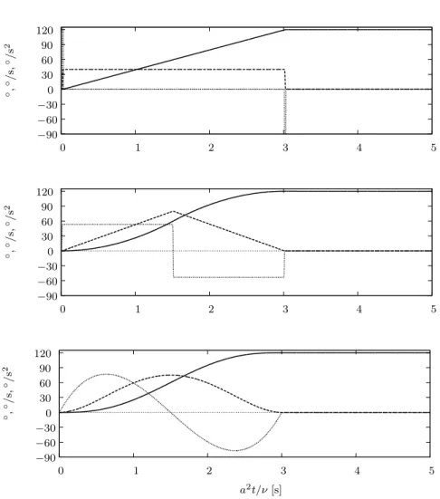
different acceleration patterns ¨α(0 ≤ a2_{t/ν ≤ 3s):} ¨ αI(t) = 2√π 9 · 0.004 " e− µ a2t/ν−0.02 0.004 ¶2 − e− µ a2t/ν−3.02 0.004 ¶2_# , ¨ αII(t) = 8 √ π 27 · 0.004 Z a2t/ν 0 h e−(τ −0.01 0.004 ) 2 − 2e−(τ −1.51 0.004 ) 2 + e−(τ −3.01 0.004 ) 2i dτ, ¨ αIII(t) = 80π 243 · (a2t/ν)3−9₂(a2t/ν)2+9 2(a 2_t/ν)¸_.

The first pattern ¨αI consists of two impulsive accelerations with opposite sign

which lead to a constant angular velocity of 40◦

/s. This pattern cannot be re-alized in a clinical test since the peak accelerations are far too high. However, its mathematical treatment is straightforward and it provides a good reference for the other patterns. The second pattern ¨αII prescribes a piecewise constant

acceleration/deceleration of 53.3◦

/s2 _{which causes a linear velocity increase up to}

80◦

/s. It is a realistic pattern in the sense that such patterns can be tested in clinical experiments using computer-controlled three-dimensional rotating chairs. The third pattern ¨αIII follows a simple polynomial function. It leads to smooth

velocity changes and comes closest to natural movements. Figure 8 shows the three patterns as functions of time.

Figure 9 shows the cupular volume displacement V⋆(t) according to (41) for the three different acceleration patterns. For small t we see that the cupular volume displacement V⋆ _{is approximately proportional to the respective angular}

velocity ˙α from Figure 8. As time progresses the velocity error ˙αe increasingly

distorts the curves in Figure 9 and V⋆ _{is now far from proportional to ˙α. In}

particular, the velocity error (42) leads to an overshoot of V⋆_{such that the cupula}

is deflected to the opposite side during the deceleration phase (for patterns II and III the overshoot starts at a2_{t/ν ≈ 2.5s). Moreover, after the head has come to}

a complete stop the cupula has not yet returned to its initial state. It returns only slowly with a fluid motion that is solely governed by the least stable mode σ0. Note that the magnitude of the overshoot is approximately independent of the

acceleration pattern.

One might expect that the overshooting of V⋆ _{would create a sensation of}

negative angular velocity since the value of V⋆ _{is beyond the threshold value V}⋆ t

that we have derived in §6.2. And indeed, such a sensation can be observed in clinical tests after a sudden deceleration following a long period of constant veloc-ity. However, we do not see it for the short Dix–Hallpike manoeuvre considered here. This apparent discrepancy between clinical experiments and our model can be explained by mechanisms of the central nerve system (see, e.g., [19]).

◦, ◦/ s, ◦/ s 2 −90 −60 −30 30 60 90 120 0 0 1 2 3 4 5 ◦, ◦/ s, ◦/ s 2 −90 −60 −30 30 60 90 120 0 0 1 2 3 4 5 ◦, ◦/ s, ◦/ s 2 a2_{t/ν [s]} −90 −60 −30 30 60 90 120 0 0 1 2 3 4 5

Figure 8. Acceleration patterns I, II & III (—— angle α, – – – angular velocity ˙α, · · · angular acceleration ¨α)

7. Conclusion

We have shown how VB’s equation (8) for the flow field in a semicircular canal can be solved analytically. We have put special emphasis on a detailed analysis of the temporal spectrum of this equation. Based on this analysis we were able to derive simple but exact expressions for the cupular volume displacement.

The simplicity of results like (41) lets us easily forget that we have not started off to our venture with a macroscopic model like Steinhausen’s torsion pendulum but rather with a partial differential equation in r and t describing the conservation of momentum in the endolymph. Only later in our work we have been able to get

V ⋆[m 3] a2_{t/ν [s]} 0.4 × 10 0 −0.4 × 10 −0.8 × 10 −1.2 × 10−12 −12 −12 −12 0 2 4 6 8 10

Figure 9. Cupular volume displacement V⋆

for the Dix-Hallpike manoeuvre (—— acceleration pattern I,– – – acceleration pattern II, · · · acceleration pattern III)

rid of explicit references to the radial coordinate r. Under this light we can split our work in three separate steps. First, we have extracted the full information on the system dynamics by finding the temporal spectrum and its corresponding eigenfunctions (§3). Second, we have condensed the modal information (§4) into the sequence {σk, κk}. With this compact information on the system dynamics

at hand we were able to forget about the particular shape of u(r, t). In a third step, we have derived the expression for the cupular volume displacement (§5) only using {σk, κk}.

It should be stressed again that the existence of both the cupular mode as well as the duct modes is required to obtain an operational semicircular canal. The fundamental difference between these modes can not only be seen from their different dependence on ǫ but also from their different behavior under the inner product (vk, Bvk). The orthogonality relation (31) shows us dramatically that

the cupular mode has a special role in the dynamics of the semicircular canal. Finally, we note that we have arrived at these results by using standard tech-niques that have been widely used in linear stability theory in general and hydro-dynamic stability in particular [22]. This work is a good example for the usefulness of these techniques not only for flows with critical stability conditions but also for highly damped flows such as the one considered in this work.

Acknowledgments

The author wishes to thank Dr. med. Stefan Hegemann of the Interdisciplinary Centre for Vertigo and Balance Disorders, Dept. of Otorhinolaryngology of the University Hospital Zurich for introducing him to the field of research on the vestibular organ, for initiating this work, and for many valuable discussions. He would also like to thank Sebastian M¨uller for his preceding work on this subject.

References

[1] Milton Abramowitz and Irene A. Stegun, Handbook of Mathematical Functions, Dover, 1965. [2] Carl M. Bender and Steven A. Orszag, Advanced Mathematical Methods for Scientists and

Engineers, McGrawHill, 1978.

[3] J. P. Bronzino, The Biomedical Engineering Handbook, CRC Press, 1995.

[4] B. Cohen, V. Matsuo, and T. Raphan, Quantitative analysis of the velocity characteristics of optokinetic nystagmus and optokinetic after-nystagmus, J. Physiol. 270 (1977), 321-344. [5] I. S. Curthoys and C. M. Oman, Dimensions of the horizontal semicircular duct, ampulla

and utricle in the human, Acta Otolaryngol. 103 (1987), 254-261.

[6] M. Dai, A. Klein, B. Cohen, and T. Raphan, Model-based study of the human cupular time constant, J. Vest. Res. 9 (1999), 293-301.

[7] E. R. Damiano and R. D. Rabbitt, A singular perturbation model of fluid dynamics in the vestibular semicircular canal and ampulla, J. Fluid Mech. 307 (1996), 333-372.

[8] M. R.Dix and C. S. Hallpike, Thepathology, symptomatology, and diagnosis of certain com-mon disorders of the vestibular system, Proc. Roy. Soc. Lond. 45 (1952), 341-354. [9] J. R. Ewald, Physiologische Untersuchungen ¨uber das Endorgan des Nervus Octavus, J. F.

Bergmann, 1892.

[10] J. J. Groen and L. B. W. Jongkees, The threshold of angular acceleration perception, J. Physiol.107 (1948), 1-7.

[11] L. H. Gustavsson, Energy growth of three-dimensional disturbances in plane Poiseuille flow, J. Fluid Mech.224 (1991), 241-260.

[12] S. M. Highstein, R. D. Rabbitt, G. R. Holstein, and R. D. Boyle, Determinants of spatial and temporal coding by semicircular canal afferents, J. Neurophysiol. 93 (2005), 2359-2370. [13] Jirair Kevorkian, Partial Differential Equations – Analytical Solution Techniques, Chapman

& Hall, 1990.

[14] R. Malcom, A quantitative study of vestibular adaptation in humans, Fourth Symposium on Role of Vestibular Organs in Space Exploration, no. NASA SP-187, 1968.

[15] J. W. McLaren and D. E. Hillman, Configuration of the cupula during endolymph pressure changes, Neurosci. Abstr. 3 (1976), 544.

[16] C. M. Oman, E. N. Marcus, and I. S. Curthoys, The influence of semicircular canal mor-phology on endolymph flow dynamics, Acta Otolaryngol. 103 (1987), 1-13.

[17] R. D. Rabbitt and E. R. Damiano, A hydroelastic model of macromechanics in the endolym-phatic vestibular canal, J. Fluid Mech. 238 (1992), 337-369.

[18] Suhrud M. Rajguru, Marytheresa A. Ifediba, and Richard D. Rabbitt, Three-dimensional biomechanical model of benign paroxysmal positional vertigo, Ann. Biomed. Eng. 32 (2004), 831-846.

[19] Th. Raphan, V. Matsuo, and B. Cohen, Velocity storage in the vestibulo-ocular reflex arc (VOR), Exp. Brain Res. 35 (1979), 229-248.

[20] D. A. Robinson, Linear addition of optokinetic and vestibular signals in the vestibular nu-cleus, Exp. Brain Res. 30 (1977), 447-450.

[21] G. Schmaltz, The physical phenomena occurring in the semicircular canals during rotary and thermic stimulation, Proc. Roy. Soc. Med. 25 (1931), 359.

[22] Peter Schmid and Dan S. Henningson, Stability and Transition in Shear Flows, Springer, 2000.

[23] W. Steinhausen, ¨Uber die Beobachtung der Cupula in den Bogengangsampullen des Labyrinths des lebenden Hechts, Pfl¨ugers Archiv f¨ur die gesamte Physiologie des Menschen und der Tiere232 (1933), 500-512.

[24] W. C. Van Buskirk, The effects of the utricle on fluid-flow in semicircular canals, Ann. Biomed. Eng.5 (1977), 1-11.

[25] W. C. Van Buskirk and J. W. Grant, Biomechanics of the semicircular canals, Biomechanics Symposium, ASME, 1973, pp. 53-54.

[26] W. C. Van Buskirk, R. G. Watts, and Y. K. Liu, The fluid mechanics of the semicircular canals, J. Fluid Mech. 78 (1976), 87-98.

[27] A. A. J. Van Egmond, J. J. Groen, and L. B. W. Jongkees, The mechanics of the semicircular canal, J. Physiol. 110 (1949), 1-11.

[28] A. Yamauchi, R. D. Rabbitt, R. Boyle, and S. M. Highstein, Relationship between inner-ear fluid pressure and semicircular canal afferent nerve discharge, JARO 3 (2001), 24-44. Dominik Obrist

Institute of Fluid Dynamics ETH Zurich

Sonneggstrasse 3 8092 Zurich Switzerland

(Received: March 16, 2006; revised: November 11, 2006 and May 26, 2007) Published Online First: October 25, 2007

To access this journal online: www.birkhauser.ch/zamp