Long-term trend of surface ozone at a regional background station in eastern China 1991?2006: enhanced variability

(1)

HAL Id: hal-00303237

https://hal.archives-ouvertes.fr/hal-00303237

Submitted on 8 Jan 2008

HAL is a multi-disciplinary open access

archive for the deposit and dissemination of sci-entific research documents, whether they are pub-lished or not. The documents may come from teaching and research institutions in France or abroad, or from public or private research centers.

L’archive ouverte pluridisciplinaire HAL, est destinée au dépôt et à la diffusion de documents scientifiques de niveau recherche, publiés ou non, émanant des établissements d’enseignement et de recherche français ou étrangers, des laboratoires publics ou privés.

Long-term trend of surface ozone at a regional

background station in eastern China 1991?2006:

enhanced variability

X. Xu, W. Lin, T. Wang, P. Yan, J. Tang, Z. Meng, Y. Wang

To cite this version:

X. Xu, W. Lin, T. Wang, P. Yan, J. Tang, et al.. Long-term trend of surface ozone at a regional background station in eastern China 1991?2006: enhanced variability. Atmospheric Chemistry and Physics Discussions, European Geosciences Union, 2008, 8 (1), pp.215-243. �hal-00303237�

(2)

ACPD

8, 215–243, 2008 Enhanced variability of surface ozone X. Xu et al. Title Page Abstract Introduction Conclusions References Tables Figures ◭ ◮ ◭ ◮ Back Close

Full Screen / Esc

Printer-friendly Version Interactive Discussion

EGU Atmos. Chem. Phys. Discuss., 8, 215–243, 2008

www.atmos-chem-phys-discuss.net/8/215/2008/ © Author(s) 2008. This work is licensed

under a Creative Commons License.

Atmospheric Chemistry and Physics Discussions

Long-term trend of surface ozone at a

regional background station in eastern

China 1991–2006: enhanced variability

X. Xu1, W. Lin1, T. Wang2, P. Yan1, J. Tang1, Z. Meng1, and Y. Wang1

1

Key Laboratory for Atmospheric Chemistry, Centre for Atmosphere Watch and Services, Chinese Academy of Meteorological Sciences, China Meteorological Administration, Beijing, China

2

Department of Civil and Structural Engineering, The Hong Kong Polytechnic University, Hong Kong, China

Received: 17 October 2007 – Accepted: 5 December 2007 – Published: 8 January 2008 Correspondence to: X. Xu (xuxb@cams.cma.gov.cn)

(3)

ACPD

Full Screen / Esc

EGU

Abstract

Information about the long-term trends of surface and tropospheric ozone is important for assessing the impact of ozone on human health, vegetation, and climate. Long-term measurements from East Asia, especially China’s eastern provinces, are urgently needed to evaluate potential changes of tropospheric ozone over this economically

5

rapid developing region. In this paper, surface ozone data from the Linan Regional Background Station in eastern China are analyzed and results about the long-term trends of surface ozone at the station are presented. Surface ozone data were col-lected at Linan during 6 periods between August 1991 and July 2006. The seasonal-ity and the long-term changes of surface ozone at the site are discussed, with focus

10

on changes in the diurnal variations, the extreme values, and the ozone distribution. Some long-term trends of surface ozone, e.g., decrease in the average concentration, increase in the daily amplitude of the relative diurnal variations, increase in the monthly highest 5% of the ozone concentration, decrease in the monthly lowest 5% of the ozone concentration, increase in the frequencies at the high and low ends of the ozone

distri-15

bution have been uncovered by the analysis. All the trends indicate that the variability of surface ozone has been enhanced. Possible causes for the observed trends are discussed. The most likely cause is believed to be the increase of NOxconcentration.

1 Introduction

Ozone is one of the key species in the atmosphere. It absorbs both solar UV and

terres-20

trial IR radiation, therefore protects living organisms at the Earth’s surface against the harmful solar UV radiation and influences the energy budget of the atmosphere (Stae-helin et al., 2001). Tropospheric ozone is one of the greenhouse gases and governs ox-idation processes in the Earth’s atmosphere through formation of OH radical (Lelieveld et al., 2000). Since OH controls the lifetime of many atmospheric species, including

25

(4)

ACPD

Full Screen / Esc

EGU consequences in atmospheric chemistry and budget of other greenhouse gases.

More-over, high level of ozone in the boundary layer exerts negative influences on the human body, agricultural crops and natural vegetation (Chameides et al., 1999; Mauzerall et al., 2005). Due to the above importance, long-term trends and the distributions of ozone in the troposphere have been intensively studied (e.g., Carslaw, 2005; Fiore et

5

al., 1998, 2002, 2005; Fusco and Logan, 2003; Gardner and Dorling, 2000; Jonson et al., 2006; Lelieveld and Dentener, 2000; Logan et al., 1999; Low and Kelly, 1992; Lu and Zhang, 2005; Menezes and Shively 2001; Naja and Akimoto, 2004; Oltmans et al., 1998, 2006; Qin et al., 2004; Simmonds et al., 2004; Tarasova et al., 2003; Vingarzan and Taylor, 2003).

10

While stratospheric ozone displayed a clear depleting trend between the late 1970s and the middle of the 1990s and some signs of recover after that (Newchurch et al., 2003; Staehelin et al., 2001; WMO, 2003), the situation regarding trends of tro-pospheric ozone is less clear. Although it is believed that global mean trotro-pospheric ozone has increased from 25 DU to 34 DU since pre-industrial era, long-term changes

15

of tropospheric ozone are highly variable and depend on region and on the time period considered (Logan et al., 1999; Oltmans et al., 1998; WMO, 2003). The differences among regions appear to be especially large for the trends of surface ozone over the past three decades. A recent review (Vingarzan, 2004) shows that the surface ozone background trend is very inconsistent among monitoring stations. An increasing trend

20

has been reported for 22 background stations, while a declining trend for 8 background stations. For many sites, no or mixed trends are reported of surface ozone (e.g., Lo-gan et al., 1999; Low and Kelly, 1992; Tarasick et al., 2005; Vingarzan, 2004; Xu et al., 1996). This inconsistence requires more observational studies in various regions, particularly those with high emissions of ozone precursors.

25

The large regional variations in ozone trends can be attributed to the large natural variability in the troposphere, but also to fewer good long-term sets of ozone measure-ments (Staehelin et al., 2001). Ozone in the surface layer is highly variable due to its short lifetime there. Therefore a dense monitoring network with well-situated

(5)

sta-ACPD

Full Screen / Esc

EGU tions is needed to obtain reliable spatial-temporal distribution of surface ozone level.

The background stations of the Global Atmosphere Watch (GAW) are suitable sites for monitoring the long-term change of surface ozone because they are usually sit-uated at places less directly influenced by anthropogenic emissions. However, the background stations are quite unevenly distributed among different parts of the world

5

(seehttp://www.empa.ch/gaw/gawsis). Most background stations with long-term mon-itoring of surface ozone are located in North America and Europe, while only a few are located in some other important parts of world, e.g., East Asia. So far, studies of long-term trends of tropospheric ozone in East Asia are mainly based on ozonesonde data over Japan (Oltmans et al., 1998; Logan et al., 1999; Naja and Akimoto, 2004)

10

and on MOZAIC aircraft data obtained in northern China (Ding et al., 2007). Long-term measurements from other parts of East Asia, especially China’s eastern provinces, are urgently needed to evaluate potential changes of tropospheric ozone over this econom-ically rapid developing region. Surface ozone has been observed at two mountain sites in East China since 2004 and data indicate that the ozone level at the sites may be

15

strongly influenced by anthropogenic sources in the surrounding areas (Li et al., 2007; Wang et al., 2006). In this paper, we present results about long-term trends of surface ozone at a background site in eastern China. We focus on the long-term changes in the variability of surface ozone at the site. Besides the trend of surface ozone level, we discuss the long-term changes of the diurnal variation of surface ozone, which have

20

seldom been touched by earlier studies.

2 Site and observations

Data used in this study were collected at the Linan Regional Background Station (30◦18′N, 119◦44′E, 139 m a.s.l.), one of the regional GAW stations in China, es-tablished and operated by China Meteorological Administration (CMA). The station

25

is located in the Yangtze Delta region, one of leading regions in economic growth in China. There are a few large cities in the E-NNW sector to Linan, with the nearest

(6)

ACPD

Full Screen / Esc

EGU and largest being Hangzhou (∼50 km easterly) and Shanghai (∼210 km northeasterly),

respectively. About 10 km to the south of the Linan station is the Linan Township with a population of approximately 50 thousands. More details about the site Linan are given in Wang et al. (2001).

To show the origins of air masses arriving at Linan, 5-day backward trajectories

5

were computed every 6 h (at 00:00, 06:00, 12:00, and 18:00 UT) for the years 2005– 2006 for 100 m above ground over Linan using the HYSPLITT 4 model (Draxler and Hess, 1997). Cluster analysis was applied to all trajectories of each season. Figure 1 displays the trajectory clusters of different seasons. In winter (December–February), the site is predominately influenced by air masses from the north. In spring (March–

10

May), nearly 50% of the air masses arriving at Linan originate from the north, 10.5% from the East China Sea, 29.2% from Shanghai and Zhejiang Province, the rest 11.2% from Southern China. In summer (June–August), nearly 70% of the air masses origi-nate from marine areas (South China Sea, Pacific Ocean, and Yellow Sea), indicating very strong effect of Asian summer monsoon. In fall (September–November), northerly

15

streams dominate and marine air masses can still be transported to the site, but not as frequent as in summer.

Continuous long-term observation of surface ozone at Linan was started on 16 July 2005. Before that time surface ozone was measured at the station for several periods. Table 1 summarizes some details of the periods with surface ozone

measure-20

ments at Linan. During these periods the Model 49 or 49C ozone analyzer from the Thermo Environmental Instruments, Inc. (TEI) or Model 1003 AH ozone analyzer from Dasibi Environmental Corp (Dashibi) have been used for the observation of surface ozone (see Table 1 for details). The TEI Model 49 and Dashibi Model 1003 AH have a lower detection limit of 2 ppbv and a precision of 2 ppbv, while the TEI Model 49C has

25

a lower detection limit of 1 ppbv and a precision of 1 ppbv. Since all these instruments are based on the reliable UV photometric technique for ozone measurement and were carefully calibrated during each period, it is unlikely that there are significant systematic differences in the measurements. The comparability of the data from different periods

(7)

ACPD

Full Screen / Esc

EGU is a prerequisite for the correctness of our results.

Raw data of surface ozone were recorded every 5 min for the period July 2005 to July 2006 and every 1 min for all other periods. Calibration data and outliers related to malfunction of the data acquisition devices or ozone analyzers were removed from the high resolution raw data. In addition, failure of electricity occurred occasionally,

5

leading to more gaps in the dataset. The estimated data capture (the number of total retained data point s divided by that of total potential data point s for each period) was in the range of 76.7%–95.0% (see Table 1). Hourly mean concentrations were calculated from the retained high resolution data and are used for further calculations in this paper.

10

3 Results and discussion

3.1 Seasonal cycle

Surface ozone at Linan varies strongly with season, as at many other rural sites. Data from four longer measurement periods (August 1994–July 1995, June 1999– December 2000, February–June 2001, and July 2005–July 2006) demonstrates that

15

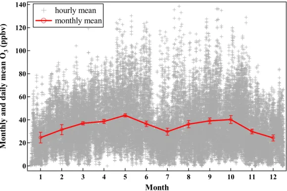
the patterns, the annual amplitudes, and positions of maxima and minima of the sonal cycles in surface ozone changed from period to period. To obtain average sea-sonal cycle the monthly mean ozone concentrations from different periods (including shorter periods) are averaged for each month of the year. Figure 2 shows the average seasonal variation. The seasonal cycle shows two peaks, with the primary being in May

20

and the secondary in October. Between the two peaks there is a valley around July. This is attributed to Asian summer monsoon, which transports maritime air masses with low ozone concentration to and causes rainy weather in the region (Wang et al., 2001, see Fig. 1). The summer valley of surface ozone concentration has been observed also at some other Eastern Asian sites (e.g., Ghim and Chang, 2000; Lam et al., 2001;

25

(8)

ACPD

Full Screen / Esc

EGU 3.2 Long-term variation of surface ozone

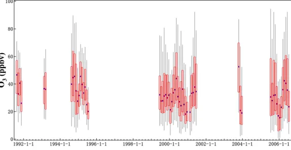
Figure 3 shows the monthly statistical results (median, 5-, 25-, 75-, and 95-percentiles) of surface ozone measured at Linan during seven periods between 1991 and 2006. As can be seen, surface ozone concentration varied in a very broad range within a month. Based on the statistics the monthly median of surface ozone concentration

5

fluctuated in the range of 15.6–52.6 ppbv, while the monthly average (not shown) varied from 17.5 ppbv to 52.3 ppbv. A trend of −(0.56±0.23) ppbv yr−1 _{for the monthly median} and a trend of −(0.37±0.23) ppbv yr−1 for the monthly average can be estimated by linear regression, suggesting that the concentration of surface ozone at Linan has been decreasing at a moderate rate. The trend for the monthly median is significant at 0.05,

10

while that for the monthly average is less significant.

The trends obtained as above should be viewed with caution as they might have been distorted by the large gaps and inhomogeneous distribution of the data points in the time series of surface ozone. Since some observation periods covered only 2–4 months and strong seasonality exits in the concentration of surface ozone at Linan (see

15

Fig. 2), there may be artifact in the estimated trends. To avoid this potential problem, data from same time periods of different years are compared as an alternative method of deriving the ozone trend. Limited by the availability of data, such comparison cannot be done for all seasons but fall and late winter. Linear trends of −(0.51±0.49) ppbv yr−1 (r2=0.26) and −(1.40±0.57) ppbv yr−1 (r2=0.67) can be obtained by applying

least-20

square fit to the average ozone concentrations for 20 August to 7 November of 1991, 1994, 1999, 2000, and 2005 and to those for February of 1993, 1995, 2000, 2001, and 2006, respectively. Although these trends are of low or moderate significance, they indicate a decreasing trend of surface ozone, in agreement with the results from the analysis of the whole dataset. Therefore it is likely that the average concentration of

25

(9)

ACPD

Full Screen / Esc

EGU 3.3 Long-term trends of diurnal variations

To see the long-term changes in the diurnal variation of surface ozone at Linan, sea-sonal average diurnal variations are calculated from the hourly mean data of the cor-responding seasons. The periods 1 March–31 May, 12 June–18 July, 1 September– 7 November and 1 December–28 February, are selected to represent spring, summer,

5

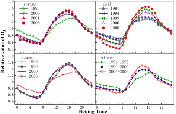
fall, and winter, respectively. It should be noted that limited by the availability of data, the periods 12 June–18 July and 1 September–7 November cover only partially sum-mer and fall days, respectively. The seasonal average diurnal variations relative to the corresponding average ozone concentrations (see Table 2) are calculated and shown in Fig. 4. As can be seen in this figure, the pattern of the average diurnal variations

10

does not change substantially from period to period. Surface ozone reaches the lowest level between 06:00 and 08:00, increases rapidly to the maximum at about 15:00, and then decreases gradually to the minimum in the early morning of next day. Similar pat-terns of diurnal variation of surface ozone were observed at many other sites, where photochemistry contributes significantly to the fluctuation of surface ozone (e.g., Ghim

15

and Chang, 2000; Saitanis, 2003; Due ˜nas, 2004; Zhang et al., 2007). The diurnal pat-terns of surface ozone at Linan, together with the large amplitudes, indicate that in all seasons photochemical formation of ozone is important in the Yangtze Delta region.

It is noteworthy that there are apparent differences between the daily amplitudes of the relative diurnal variations for different years. The spring data in Fig. 4 show the

20

lowest daily amplitude in 1995, a large increase of the daily amplitude from 1995 to 2000, and a small increase from 2000 to 2001 and 2006. The summer diurnal cycles of surface ozone and their daily amplitudes in 1999, 2000, and 2006 look very similar and clearly different from those in 1995. The peak and valley positions of the diurnal variation of surface in 1995 appeared later and the daily amplitude was much smaller

25

than those in the other years. The fall daily amplitude changed little from 1991 to 1994, increased significantly to 1999 and 2000, and reached the highest in 2006. The winter data in Fig. 4 show a gradual and significant increase in the daily amplitude from

(10)

ACPD

Full Screen / Esc

EGU 1994–1995 to 1999–2000 and to 2005–2006.

Figure 5 shows the long-term changes in the daily maximum and minimum of the relative diurnal variations of surface ozone at Linan, displaying in another way the in-crease tendency in the daily amplitude of surface ozone. As can be seen from Fig. 3, in all seasons the maximum of the relative diurnal variation has been increasing and the

5

minimum decreasing. Linear trends of the maximum and minimum values are obtained by applying least-square fit to the data. The maximum value shows increase rates of 2.0% yr−1_{(α<0.2), 2.7% yr}−1 _{(α>0.2), 2.4% yr}−1_{(α<0.05), and 2.0% yr}−1_{(α<0.05) for} spring, summer, fall, and winter, respectively. The minimum value shows decrease rates of 0.8% yr−1 (α>0.2), 2.5% yr−1 (α<0.1), 1.8% yr−1 (α<0.05), and 0.6% yr−1

10

(α<0.05) for spring, summer, fall, and winter, respectively.

In summary, some long-term changes in the diurnal variations of surface ozone at Linan have occurred since the early 1990s. These changes are (1) increase of the rel-ative diurnal maximum, (2) decrease of the relrel-ative diurnal minimum, and (3) increase of the daily amplitude of surface ozone in all seasons. In other words, the variability

15

of surface ozone at Linan has been enhanced over the last 15 years, with the daily maximum of surface ozone getting higher and the daily minimum getting lower.

3.4 Long-term trend of extreme values

In the previous section the long-term changes in the variability of surface ozone at Linan are demonstrated using the data of relative diurnal variation. In this section, the

20

long-term changes are illustrated using the observed extreme values of surface ozone at the station. Values greater than the 95-percentile of the hourly mean ozone concen-trations in a month are averaged to obtain the average of the monthly highest 5%, while values lower than the 5-percentile are averaged to obtain the average of the monthly lowest 5%. Nearly 96% of the values greater than the 95-percentiles occurred in

day-25

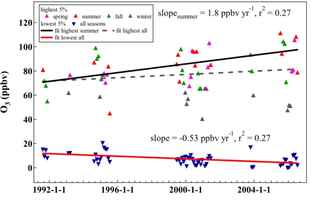
time (Beijing Time 08:00–20:00) and 86% of the values lower than the 5-percentiles occurred during the night (Beijing Time 20:00–08:00). Figure 6 shows the averages of the monthly highest 5% and lowest 5% of the hourly mean ozone concentrations at

(11)

ACPD

Full Screen / Esc

EGU Linan. As can be seen in the figure, the data points are much scattering, especially

those of the monthly highest 5%, nevertheless, we performed least-square fitting to the data to obtain the trends of both types of extreme values. The slopes of the two regression lines (gray dashed line and red solid line in Fig. 6) indicate that the high-est and lowhigh-est values of surface ozone at Linan have different trends. The average of

5

the monthly highest 5% has increased at a rate of 0.68 ppbv yr−1, while the average of the monthly lowest 5% has decreased at a rate of 0.53 ppbv yr−1. It should be noted that the trend of the highest 5% values is less significant (α>0.05) due to strong varia-tions in the values. Inspecting the colored points of the highest 5% values for different seasons, one can recognize that the larger scattering can be attributed partly to the

10

seasonal differences. The winter values are far apart from the group. While data from other seasons show an increasing trend, the winter data show a decreasing trend of 1.4 ppbv yr−1(α<0.05). The most rapid increase has occurred in the monthly highest 5% in summer, with a rate of 1.8 ppbv yr−1 _(α<0.05).

In consequence of the above long-term changes the distribution of the concentration

15

of surface ozone at Linan has changed significantly since about a decade. Figure 7 shows the distributions of the hourly mean concentrations of surface ozone at Linan, for the 1994–1995, 1999–2001, and 2005–2006 periods, respectively. Effective hourly mean data points from periods 1994–1995, 1999–2001, and 2005–2006 are 6325, 14 677, and 8779, respectively. As can be seen in Fig. 7 and the blowup in it, the

left-20

most part of the distribution curve has shifted towards left and the rightmost towards right, suggesting that both extreme low and extreme high concentrations have become more frequent and the ozone concentration has become more variable. It is also note-worthy that the shift towards the low end of the distribution was stronger than the shift towards the high end, i.e., more and more data points are distributed in the lower ozone

25

concentration range and less and less in the higher ozone concentration range. In con-sequence of these shift, the peak of the distribution curve of surface ozone has shifted towards lower value despite an increase in variance of ozone concentration.

(12)

ACPD

Full Screen / Esc

EGU 3.5 Possible causes for the observed long-term trends

Surface ozone is closely related to many processes, such as photochemistry, dry de-position, transport, etc. It is well known that NO_x are key species for the variation of tropospheric ozone. In the presence of sufficient sunlight NOx catalyze the photo-chemical oxidation of VOCs and other species to form ozone. During nighttime and in

5

the cold seasons with no or less intensive sunlight NOxremove ozone through titration reaction, in which NO reacts with ozone to form NO₂. Therefore changes in the NO_x emission may have different effects on the variability of surface ozone, depending on time and location. Theoretically, if other conditions remain stable, a larger or smaller NO_xemission can lead to enhancement or reduction in the variability of surface ozone.

10

Indeed a few studies (e.g., Lefohn et al., 1998; Lin et al., 2000; TOR-2, 2003; Solberg et al., 2004; Ord ´o ˜nez et al., 2005; Chou et al., 2006; Jonson et al., 2006) show either a decrease in high ozone concentrations or an increase in low ozone concentrations or both, consistent with the local decline in NOx emission. These changes reduce the variability of surface ozone. To our best knowledge there has been virtually no previous

15

study showing enhancement in the variability of surface ozone at background site as a result of increasing NOx level. We believe that the enhanced variability of surface ozone shown in Sect. 3.3 and 3.4 is such an example.

The Yangtze Delta region, in which Linan is located, is one of most densely popu-lated and industrialized regions in China. Booming economy in and outside the region

20

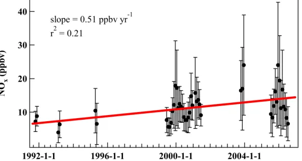
has been causing significant increase in the emissions of some key pollutants (Streets et al., 2003). As a result, the atmospheric concentrations of the pollutants have been increasing. Richter et al. (2005) and Zhang et al. (2007) report a large increase of the tropospheric column of NO2over East Central China. In situ measurements show that NO_x concentration at Linan has been increasing since 1992, as shown in Fig. 8. In

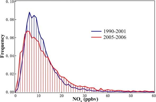
25

addition, there have been some changes in the frequency distribution of the NOx con-centration. The frequency distributions of the hourly mean NOxconcentration from the periods 1999–2001 and 2005–2006 are displayed in Fig. 9. They look similar but differ

(13)

ACPD

Full Screen / Esc

EGU in details. The frequencies of lower and higher NO_xconcentrations during 2005–2006

were higher than those during 1991–2001, while frequencies of the concentrations around median during 2005–2006 were lower than those during 1991–2001. The over-all effect of above changes in the frequency distribution is an increase of the average NOx concentration, from 11.1 ppbv in 1999–2001 to 13.4 ppbv in 2005–2006. The

in-5

crease rate of NOx concentration at Linan is estimated to be 0.51 ppbv yr−1 (Fig. 8). Interestingly, this NOx trend is close to the decrease rate of the monthly lowest 5% and the increase rate of the monthly highest 5% of ozone concentration (see Fig. 6). From August 1999 to July 2006 the NOxconcentration at Linan increased at a rate of about 3.2%. This growth rate is large enough to have significant impacts on surface

10

ozone. Luo et al. (2000) pointed out that ozone formation in rural areas in the Yangtze Delta region is NOx-limited. Wang et al. (2001) reported a positive correlation between ozone and NOx during afternoon hours at Lin’an in summer months, providing obser-vational evidence for the NO_x-limited chemistry. Therefore the increasing trend of NO_x may have caused more daytime production of ozone, especially during warmer months,

15

and more titration of ozone during nighttime and cold months. These effects are con-sistent with the phenomena discussed in Sects. 3.3 and 3.4. Hence it is likely that the observed long-term trends in the variability of surface ozone at Linan are mainly caused by the increase of NOxconcentration in the Yangtze Delta region.

It should be noted that some other factors may also have contributed to the changes

20

in the variability of surface ozone. These factors include increasing emission of NMHCs, stratospheric ozone depletion, etc. Indeed measurements show that the total concentration of NMHCs at Linan doubled in the last decade (Xu et al., 1996; Wang et al., 2006). The increase of NMHCs concentration may have contributed to more pho-tochemical production of ozone. However, it is unlikely that this increase have caused

25

a significant decreasing trend of the low end of the ozone distribution. The tempera-ture at Linan has been quite stable (with change <0.008◦C yr−1) since 1991, so that it cannot be a cause of the trend in the variability of surface ozone. Secular changes (if any) in transport and dry deposition of ozone would have influenced the ozone

(14)

con-ACPD

Full Screen / Esc

EGU centration at Linan. However, it is unclear whether or not such changes have occurred.

Moreover, it seems to be unlikely that the changes in transport and dry deposition can explain all the trends shown in Sects. 3.3 and 3.4.

4 Conclusions

In this paper we present some long-term trends of the features of surface ozone at

5

Linan including: a decrease in the average concentration, an increase in the daily am-plitude of the relative diurnal variation, an increase in the monthly highest 5% and a decrease in the monthly lowest 5% of the ozone concentration, and an increase in the frequencies at the high and low ends of the ozone distribution. All the trends indicate that the variability of surface ozone has been enhanced. We believe that the enhanced

10

variability of surface ozone is mainly caused by an increase of NO_x concentration or emission in the Yangtze Delta region, in which Linan is located. Because this study is based on the intermittent measurements made during several periods in the last 15 years, modeling studies are needed to better understand the observed trends and their causes. The increase in the extreme high concentration may have negative

im-15

pact on human health and vegetation and can also change the oxidizing capacity on which atmospheric chemistry highly depends. Therefore monitoring of surface ozone at the site should be continued and control measures should be taken to avoid further exacerbation of ozone pollution.

Acknowledgements. We thank the staff of the Linan station for carrying out the measurements.

20

This work is supported by the CMA project (CCSF2005-3-DH02) and the “National Basic Re-search Program of China” (No. 2005CB4222002 and 2005CB4222003). X. Xu thanks the grant from the Ministry of Personnel of the People’s Republic of China.

(15)

ACPD

Full Screen / Esc

EGU

References

Carslaw, D. C.: On the changing seasonal cycles and trends of ozone at Mace Head, Ireland, Atmos. Chem. Phys., 5, 3441–3450, 2005,

http://www.atmos-chem-phys.net/5/3441/2005/.

Chameides, W. L., Li, X., Tang, X., Zhou, X., Luo, C., Kiang, C. S., John, J. St., Saylor, R. D.,

5

Liu, S. C., Lam, K. S., Wang, T., and Giorgi, F.: Is ozone pollution affecting crop yields in China, Geophys. Res. Lett., 26, 867–870, 1999.

Chou, C. C.-K., Liu, S. C., Lina, C.-Y., Shiu, C.-J., and Chang, K.-H.: The trend of surface ozone in Taipei, Taiwan, and its causes: Implications for ozone control strategies, Atmos. Environ., 40, 3898–3908, 2006.

10

Ding, A. J., Wang, T., Thouret, V., Cammas, J.-P., and Nedelec, P.: Tropospheric ozone cli-matology over Beijing: analysis of aircraft data from the MOZAIC program, Atmos. Chem. Phys., 8, 1–13, 2008,http://www.atmos-chem-phys.net/8/1/2008/.

Draxler, R. R. and Hess, G. D.: Description of the HYSPLIT 4-modeling system, NOAA Tech. Memo. ERL ARL-224, NOAA, Silver Spring, Md., 24 pp., 1997.

15

Due ñas, C., Fern ández, M.C., Ca ñete, S., Carretero, J., and Liger, E.: Analyses of ozone in urban and rural sites in M álaga (Spain), Chemosphere, 56, 631–639, 2004.

Fiore, A. M., Jacob, D. J., Logan, J. A., and Yin, J. H.: Long-term trends in ground level ozone over the contiguous United States, 1980–1995, J. Geophys. Res., 103(D1), 1471–1480, 1998.

20

Fiore, A. M., Jacob, D. J., Bey, I., Yantosca, R. M., Field, B. D., and Fusco A. C.: Background ozone over the United States in summer: origin, trend, and contribution to pollution episodes, J. Geophys. Res., 107(D15), doi:10.1029/2001JD000982, 2002.

Fiore, A. M., Horowitz, L. W., Purves, D. W., Levy II, H., Evans, M. J., Wang, Y., Li, Q., and Yantosca, R. M.: Evaluating the contribution of changes in isoprene emissions to

25

surface ozone trends over the eastern United States, J. Geophys. Res., 110, D12303, doi:10.1029/2004JD005485, 2005.

Fusco, A. C. and Logan, J. A.: Analysis of 1970–1995 trends in tropospheric ozone at Northern Hemisphere midlatitudes with the GEOS-CHEM model, J. Geophys. Res., 108(D15), 4449, doi:10.1029/2002JD002742, 2003.

30

Gardner, M. W. and Dorling, S. R.: Meteorologically adjusted trends in UK daily maximum surface ozone concentrations, Atmos. Environ., 34, 171–176, 2000.

(16)

ACPD

Full Screen / Esc

EGU Ghim, Y. S. and Chang, Y.-S.: Characteristics of ground-level ozone distributions in Korea for

the period of 1990–1995, J. Geophys. Res., 105(D7), 8877–8890, 2000.

Jonson, J. E., Simpson, D., Fagerli, H., and Solberg, S.: Can we explain the trends in European ozone levels?, Atmos. Chem. Phys., 6, 51–66, 2006,

5

Lam, K. S., Wang, T. J., Chan, L. Y., Wang, T., and Harris, J.: Flow patterns influencing the seasonal behavior of surface ozone and carbon monoxide at a coastal site near Hong Kong, Atmos. Environ., 35, 3121–3135, 2001.

Lefohn, A. S., Shadwick, D. S., and Ziman, S. D.: The difficult challenge of attaining EPA’s new ozone standard, Environ. Sci. Technol., 32, 276A–282A, 1998.

10

Lelieveld, J. and Dentener, F. J.: What controls tropospheric ozone? J. Geophys. Res., 105(D3), 3531–3551, 2000.

Li, J., Wang, Z., Akimoto, H., Gao, C., Pochanart, P., and Wang, X.: Modeling study of ozone seasonal cycle in lower troposphere over east Asia, J. Geophys. Res., 112, D22S25, doi:10.1029/2006JD008209, 2007.

15

Lin, C.-Y. C, Jacob, D. J., Munger, J. W., and Fiore, A. M.: Increasing background ozone in surface air over the United States, Geophys. Res. Lett., 27(21), 3465–3468, 2000.

Logan, J. A., Megretskaia, I. A., Miller, A. J., Tiao, G. C., Choi, D., Zhang, L., Stolarski, R. S., Labow, G. J., Hollandsworth, S. M., Bodeker, G. E., Claude, H., De Muer, D., Kerr, J. B., Tarasick, D. W., Oltmans, S. J., Johnson, B., Schmidlin, F., Staehelin, J., Viatte, P., and

20

Uchino, O.: Trends in the vertical distribution of ozone: A comparison of two analyses of ozonesonde data, J. Geophys. Res., 104, 26 373–26 399, 1999.

Low, P. S. and Kelly, P. M.: Variations in surface ozone trends over Europe, Geophys. Res. Lett., 19(11), 1117–1120, 1992.

Lu, H.-C. and Chang, T.-S.: Meteorologically adjusted trends of daily maximum ozone

concen-25

trations in Taipei, Taiwan, Atmos. Environ., 39, 6491–6501, 2005.

Luo, C., Ding, G., Li, X., Tang, J., and Zhou, X.: Preliminary analysis and comparison of results in field experiment of Sino-US atmospheric chemical cooperation investigation: PEM-WEST B, Acta Meteorol. Sinica, 56(4), 467–475, 1998.

Luo, C., St. John, J. C., Zhou, X. J., Lam, K. S., Wang, T., and Chameides, W. L.: A nonurban

30

ozone air pollution episode over eastern China: Observations and model simulations, J. Geophys. Res., 105, 1889–1908, 2000.

(17)

ACPD

Full Screen / Esc

EGU sources: variability in ozone production, resulting health damages and economic costs,

At-mos. Environ., 39, 2851–2866, 2005.

Menezes, K. A. and Shively, T. S.: Estimating the Long-term Trend in the Extreme Values of Tropospheric Ozone Using a Multivariate Approach, Environ. Sci. Technol., 35, 2554–2561, 2001.

5

Naja, M. and Akimoto, H.: Contribution of regional pollution and long-range transport to the Asia-Pacific region: Analysis of long-term ozonesonde data over Japan, J. Geophys. Res., 109, 1306, doi:10.1029/2004JD004687, 2004.

Newchurch, M. J., Yang, E.-S., Cunnold, D. M., Reinsel, G. C., Zawodny, J. M., and Russell III, J. M.: Evidence for slowdown in stratospheric ozone loss: First stage of ozone recovery, J.

10

Geophys. Res., 108(D16), 4507, doi:10.1029/2003JD003471, 2003.

Oltmans, S. J., Lefohn, A. S., Sheel, H. E., Harris, J. M., Levy, H., Galbally, I. E., Brunke, E.-G., Meyer, C. P., Lathrop, J. A., Johnson, B. J., Shadwick, D. S., Cuevas, E., Schmidlin, F. J., Tarasick, D. W., Claude, H., Kerr, J. B., Uchino, O., and Mohnen, V.: Trends of ozone in the troposphere, Geophys. Res. Lett., 25, 139–142, 1998.

15

Oltmans, S. J., Lefohn, A. S., Harris, J. M., Galbally, I., Scheel, H. E., Bodeker, G., Brunke, E., Claude, H., Tarasick, D., Johnson, B. J., Simmonds, P., Shadwick, D., Anlauf, K., Hayden, K., Schmidlin, F., Fujimoto, T., Akagi, K., Meyer, C., Nichol, S., Davies, J., Redondas, A., and Cuevas, E.: Long-term changes in tropospheric ozone, Atmos. Environ., 40, 3156–3173, 2006.

20

Ord ó ñez, C., Mathis, H., Furger, M., Henne, S., H üglin, C., Staehelin, J., and Pr év ôt, A. S. H.: Changes of daily surface ozone maxima in Switzerland in all seasons from 1992 to 2002 and discussion of summer 2003, Atmos. Chem. Phys., 5, 1187–1203, 2005,

Pochanart, P., Akimoto, H., Kinjo, Y., and Tanimoto, H.: Surface ozone at four remote island

25

sites and the preliminary assessment of the exceedances of its critical level in Japan, Atmos. Environ., 36, 4235–4250, 2002.

Qin, Y., Tonnesen, G. S., and Wang, Z.: One-hour and eight-hour average ozone in the Cali-fornia South Coast air quality management district: trends in peak values and sensitivity to precursors, Atmos. Environ., 38, 2197–2207, 2004.

30

Richter, A., Burrows, J. P., Nuß, H., Granier, C., and Niemeier, U.: Increase in tro-pospheric nitrogen dioxide over China observed from space, Nature, 437(1), 129–132, doi:10.1038/nature04092, 2005.

(18)

ACPD

Full Screen / Esc

EGU Saitanis, C. J.: Background ozone monitoring and phytodetection in the greater rural area of

Corinth – Greece, Chemosphere, 51, 913–923, 2003.

Simmonds, P. G., Derwent, R. G., Manningc, A. L., and Spain, G.: Significant growth in surface ozone at Mace Head, Ireland, 1987–2003, Atmos. Environ., 38, 4769–4778, 2004.

Solberg, S., Simpson, D., Jonson, J., Hjellberekke, A., and Derwent, R.: Ozone, in: EMEP

5

assessment PART I: European perspective, edited by: Løvblad, G., Tarras ´on, L., Tørseth, K., and Dutchak, S., Tech. Rep., The Norwegian Meteorological Institute, Oslo, Norway, 2004.

Staehelin, J., Harris, N. R. P., Appenzeller, C., and Eberhard, J.: Ozone Trends: A Review, Rev. Geophys., 39(2), 231–290, 2001.

10

Streets, D. G., Bond, T. C., Carmichael, G. R., Fernandes, S. D., Fu, Q., He, D., Klimont, Z., Nel-son, S. M., Tsai, N. Y., Wang, M. Q., Woo, J.-H., and Yarber, K. F.: An inventory of gaseous and primary aerosol emissions in Asia in the year 2000, J. Geophys. Res., 108(D21), 8809, doi:10.1029/2002JD003093, 2003.

Tarasick, D. W., Wardle, D. I., Kerr, J. B., Bellefleur, J. J., and Davies, J.: Tropospheric ozone

15

trends over Canada: 1980–1993, Geophys. Res. Lett., 22, 409–412, 1995.

Tarasova, O. A., Elansky, N. F., Kuznetsov, G. I., Kuznetsova, I. N., and Senik, I. A.: Impact of Air Transport on Seasonal Variations and Trends of Surface Ozone at Kislovodsk High Mountain Station, J. Atmos. Chem., 45, 245–259, 2003.

TOR-2: Tropospheric Ozone Research, EUROTRAC-2 Subproject Final Report, ISS

GSF-20

National Research Center for Environment and Health, Munich, Germany, 2003.

Vingarzan, R.: A review of surface ozone background levels and trends, Atmos. Environ., 38, 3431–3442, 2004.

Vingarzan, R. and Taylor, B.: Trend analysis of ground level ozone in the greater Vancou-ver/Fraser Valley area of British Columbia, Atmos. Environ., 37, 2159–2171, 2003.

25

Wang, H., Tang, X., Wang, M., Yan, P., Wang, T., Shao, K., Zeng, L., Du, H., and Chen, L.: Characteristics of observed trace gaseous pollutants in the Yangtze Delta, Science in China (D), 46(4), 297–404, 2003.

Wang, M., Cheng, H., Ding, G., Tang, J., Yu, X., Liu, G., and Zhou, H.: Study on the compo-sition of NMHCs and the variation of concentration at Linan and Shangdianzi atmospheric

30

background station, Acta Meteorol. Sinica, 64(5), 658–665, 2006.

Wang, T., Cheung, V. T. F., Anson, M., and Li, Y. S.: Ozone and related gaseous pollutants in the boundary layer of eastern China: Overview of the recent measurements at a rural site,

(19)

ACPD

Full Screen / Esc

EGU Geophys. Res. Lett., 28(12), 2373–2376, 2001.

Wang, T., Wong, C. H., Cheung, T. F., Blake, D. R., Arimoto, R., Baumann, K., Tang, J., Ding, G. A., Yu, X. M., Li, Y. S., Streets, D. D., and Simpson, I. J.: Relationships of trace gases and aerosols and the emission characteristics at Lin’an, a rural site in eastern China during spring 2001, J. Geophys. Res., 109, D19S05, doi:10:1029/2003JD004119, 2004.

5

Wang, Z., Li, J., Wang, X., Pochanart, P., and Akimoto, H.: Modeling of Regional High Ozone Episode Observed at Two Mountain Sites (Mt. Tai and Huang) in East China, J. Atmos. Chem., 55(3), doi:10.1007/s10874-006-9038-6, 253–272, 2006.

WMO: Scientific Assessment of Ozone Depletion: 2002, Global Ozone Research and Monitor-ing Project-Report No. 47, Geneva, 2003.

10

Xu, X., Xian, Y., Ding, G., and Li, X.: Continental background NMHC concentration, compo-sition, and relation to surface ozone, in: Atmospheric Ozone Variations and Its Effect on the Climate and Environment in China, edited by: Zhou, X., Meteorological Press, Beijing, 67–81, 1996.

Xu, D., Yap, D., and Taylor, P.A.: Meteorologically adjusted ground level ozone trends in Ontario,

15

Atmos. Environ., 30(7), 1117–1124, 1996.

Yamaji, K., Ohara, T., Uno, I., Tanimoto, H., Kurokawa, J., and Akimoto, H.: Analysis of the seasonal variation of ozone in the boundary layer in East Asia using the Community Multi-scale Air Quality model: What controls surface ozone levels over Japan?, Atmos. Environ., 40, 1856–1868, 2006.

20

Yan, P., Li, X., Luo, C., Xu, X., Xiang, Y., Ding, G., Tang, J. , Wang, M., and Yu, X.: Observational analysis of surface O₃, NO_xand SO₂in China, Quart. J. Appl. Meteor., 8(1), 53–60, 1997. Zhang, J., Wang, T., Chameides, W. L., Cardelino, C., Kwok, J., Blake, D. R., Ding, A., and So,

K. L.: Ozone production and hydrocarbon reactivity in Hong Kong, Southern China, Atmos. Chem. Phys., 7, 557–573, 2007,

25

Zhang, X., Zhang, P., Zhang, Y., Li, X., and Qiu, H.: The trend, seasonal cycle, and sources of tropospheric NO₂over China during 1996∼2006 based on satellite measurement, Science in China (D), 50(12), 1877–1884, 2007.

Zhou, X., Luo, C., Ding, G., Tang, J., and Liu, Q.: Preliminary study of background variations

30

of atmospheric ozone and its precursors over eastern China, Science in China (B), 24(12), 1323–1330, 1994.

(20)

ACPD

Full Screen / Esc

EGU

Table 1. Periods with surface ozone data analyzed in this paper.

Period Project Ozone analyzer Data capture Data source / Reference (precision)

Aug. 1991 to PEM-WEST A TEI Model 49 1 min, 95.0% http://www-gte.larc.nasa.gov/

Nov. 1991 (2 ppbv) Zhou et al. (1994) Feb. 1993 to PEM-WEST B TEI Model 49 1 min, 94.6% http://www-gte.larc.nasa.gov/

Mar. 1993 (2 ppbv) Luo et al. (1998) Aug. 1994 to Chinese Ozone Dashibi Model 1 min, 78.4% Yan, et al. (1997) July 1995 Research Program 1003AH

(CORP) (2 ppbv)

June 1999 to China-MAP TEI Model 49 1 min, 79.3% Wang et al. (2001)

June 2000 (2 ppbv)

Wang et al. (2003) July 2000 to ACE-Asia TEI Model 49C 1 min, 76.7% Wang et al. (2004)

June 2001 (1 ppbv) and

Wang and Tang (unpublished data) Oct. 2003 to Study of TEI Model 49 C 1 min, 94.2% Tang Dec. 2003 Continental (1 ppbv) (unpublished

Atmospheric Background data) (SCAB)

July 2005 to Operational TEI Model 49 C 5 min, 91.1% This work July 2006 long-term (1 ppbv)

(21)

ACPD

Full Screen / Esc

EGU

Table 2. Average ozone concentrations in different seasons and years.

year spring summer fall winter

1991 37.8 1994 49.2 1994–1995 36.0 1995 40.0 21.7 1999 33.7 35.6 1999–2000 28.4 2000 40.2 32.8 33.0 2001 38.3 2005 38.4 2005–2006 19.8 2006 41.8 33.5

(22)

ACPD

Full Screen / Esc

EGU

Fig. 1. Seasonal variation of air mass backward trajectories at Linan. Trajectory clusters for

winter (left up), spring (right up), summer (left bottom), and fall (right bottom) are calculated based on the trajectories of 2005–2006. 72-hour trajectories are shown with steps of 12 hours. The proportions of different clusters are given in the colored boxes.

(23)

ACPD

Full Screen / Esc

Printer-friendly Version Interactive Discussion EGU 140 120 100 80 60 40 20 0 M o n th ly an d d ai ly me a n O 3 (p p b v ) 12 11 10 9 8 7 6 5 4 3 2 1 Month hourly mean monthly mean

Fig. 2. Average seasonal cycle of surface ozone at Linan. The red circles indicate climatology

monthly mean concentrations calculated from the monthly mean ozone concentrations of the same months of different years. The vertical bars represent one standard deviation of the climatology monthly mean concentrations. The grey crosses represent hourly mean ozone concentrations from all periods listed in Table 1.

(24)

ACPD

Full Screen / Esc

Printer-friendly Version Interactive Discussion EGU 100 80 60 40 20 0 O3 (p p b v) 199 2-1-1 1 994-1-1 199 6-1-1 1 998-1- 1 200 0-1-1 2 002-1- 1 200 4-1-1 2 006-1- 1

Fig. 3. Variations of monthly median (blue dash), 5-percentiles (whisker bottom), 25-percentile

(box bottom), 75-percentile (box top), and 95-percentile (whisker top) of surface ozone concen-trations observed at Linan during different periods.

(25)

ACPD

Full Screen / Esc

Printer-friendly Version Interactive Discussion EGU 1 . 8 1 . 6 1 . 4 1 . 2 1 . 0 0 . 8 0 . 6 0 . 4 R e lat ive val u e of O 3 2 0 1 6 1 2 8 4 0 1 . 8 1 . 6 1 . 4 1 . 2 1 . 0 0 . 8 0 . 6 0 . 4 2 0 1 6 1 2 8 4 0 Beijing Time spring 1995 2000 2001 2006 summer 1995 1999 2000 2006 fall 1991 1994 1999 2000 2005 winter 1994-1995 1999-2000 2005-2006

Fig. 4. Relative diurnal variations of surface ozone at Linan in spring (up-left), summer

(bottom-left), fall (up-right), and winter (bottom-right) of different years. Each curve in the figure repre-sents a seasonal average diurnal variation relative to the average ozone concentration of the corresponding season and year (see Table 2), so that the values are dimensionless.

(26)

ACPD

Full Screen / Esc

Printer-friendly Version Interactive Discussion EGU 1 .8 1 .6 1 .4 1 .2 1 .0 0 .8 0 .6 0 .4 R el a ti ve v a lu e of O 3 2006 2 004 20 02 200 0 1 998 19 96 199 4 1992 1990 1 .8 1 .6 1 .4 1 .2 1 .0 0 .8 0 .6 0 .4 20 06 200 4 2 002 20 00 199 8 1996 199 4 1992 1990 spring daily maximum daily minimum fall daily maximum daily minimum summer daily maximum daily minimum winter daily maximum daily minimum 2.0% yr-1, r2 = 0.67 -0.8% yr-1, r2 = 0.55 2.7% yr-1, r2 = 0.61 -2.5% yr-1, r2 = 0.86 2.4% yr-1, r2 = 0.82 -1.8% yr-1, r2 = 0.81 1.9% yr-1, r2 = 1.00 -0.6% yr-1, r2 = 1.00

Fig. 5. Long-term changes in the daily maximum and minimum of the relative diurnal

varia-tions of surface ozone at Linan in different seasons. The daily maximum and minimum values represent the peaks and valleys of the seasonal average diurnal variations of surface ozone in Fig. 4.

(27)

ACPD

Full Screen / Esc

Printer-friendly Version Interactive Discussion EGU 120 100 80 60 40 20 0

O

3

(p

p

b

v

)

1992-1-1 1996-1-1 2000-1-1 2004-1-1 slope_summer = 1.8 ppbv yr-1, r2 = 0.27 slope = -0.53 ppbv yr-1, r2 = 0.27 highest 5%

spring summer fall winter

lowest 5% all seasons

fit highest summer fit highest all fit lowest all

Fig. 6. Long-term changes in averages of the monthly highest 5% and lowest 5% of surface

(28)

ACPD

Full Screen / Esc

Printer-friendly Version Interactive Discussion EGU 0.06 0.05 0.04 0.03 0.02 0.01 0.00

Frequency

150 100 50 0

O

₃

(ppbv)

1994-1995 1999-2001 2005-2006 0.005 0.004 0.003 0.002 0.001 0.000 180 160 140 120 100 80

Fig. 7. Distributions of the hourly mean concentrations of surface ozone at Linan, for the

periods 1994–1995, 1999–2001 and 2005–2006. The frequencies are values relative to the total numbers of data points from different periods (see text for details). The blow-up shows the details of the right tails of the distributions. The blue and red arrows indicate the respective shift directions of the leftmost and rightmost parts of the distribution curves, and the black arrow indicates the shift direction of the peak of the distribution curves.

(29)

ACPD

Full Screen / Esc

Printer-friendly Version Interactive Discussion EGU

40

30

20

10 N

O

x

(p

p

b

v)

1992-1-1

1996-1-1

2000-1-1

2004-1-1

slope = 0.51 ppbv yr

-1

r

2

= 0.21

Fig. 8. Monthly mean NO_x concentration at Linan. The vertical bars represent the standard deviation of the monthly mean concentration.

(30)

ACPD

Full Screen / Esc

Printer-friendly Version Interactive Discussion EGU 0.10 0.08 0.06 0.04 0.02 0.00

F

r

e

q

u

e

n

c

y

60 50 40 30 20 10 0

NO

_x

(ppbv)

1990-2001

2005-2006

Fig. 9. Distributions of the hourly mean concentrations of NO_xat Linan for the periods 1999– 2001 and 2005–2006.