HAL Id: hal-01645456
https://hal.archives-ouvertes.fr/hal-01645456
Submitted on 3 May 2018
HAL is a multi-disciplinary open access
archive for the deposit and dissemination of
sci-entific research documents, whether they are
pub-lished or not. The documents may come from
teaching and research institutions in France or
abroad, or from public or private research centers.
L’archive ouverte pluridisciplinaire HAL, est
destinée au dépôt et à la diffusion de documents
scientifiques de niveau recherche, publiés ou non,
émanant des établissements d’enseignement et de
recherche français ou étrangers, des laboratoires
publics ou privés.
The COSMOS2015 galaxy stellar mass function
-Thirteen billion years of stellar mass assembly in ten
snapshots
I. Davidzon, O. Ilbert, C. Laigle, J. Coupon, H.J. Mccracken, I. Delvecchio, D.
Masters, P. Capak, B.C. Hsieh, O. Le Fèvre, et al.
To cite this version:
I. Davidzon, O. Ilbert, C. Laigle, J. Coupon, H.J. Mccracken, et al.. The COSMOS2015 galaxy stellar
mass function - Thirteen billion years of stellar mass assembly in ten snapshots. Astron.Astrophys.,
2017, 605, pp.A70. �10.1051/0004-6361/201730419�. �hal-01645456�
May 25, 2017
The COSMOS2015 galaxy stellar mass function
?
13 billion years of stellar mass assembly in 10 snapshots
I. Davidzon
1, 2, O. Ilbert
1, C. Laigle
3, J. Coupon
4, H. J. McCracken
5, I. Delvecchio
6, D. Masters
7, P. L. Capak
7,
B. C. Hsieh
8, O. Le Fèvre
1, L. Tresse
9, M. Bethermin
1, Y.-Y. Chang
8, 10, A. L. Faisst
7, E. Le Floc’h
10, C. Steinhardt
11,
S. Toft
11, H. Aussel
10, C. Dubois
1, G. Hasinger
12, M. Salvato
13, D. B. Sanders
12, N. Scoville
14, and J. D. Silverman
15(Affiliations can be found after the references) January 2017
ABSTRACT
We measure the stellar mass function (SMF) and stellar mass density of galaxies in the COSMOS field up to z ∼ 6. We select them in the near-IR bands of the COSMOS2015 catalogue, which includes ultra-deep photometry from UltraVISTA-DR2, SPLASH, and Subaru/Hyper Suprime-Cam. At z > 2.5 we use new precise photometric redshifts with error σz= 0.03(1+z) and an outlier fraction of
12%, estimated by means of the unique spectroscopic sample of COSMOS (∼ 100 000 spectroscopic measurements in total, more than thousand with robust zspec> 2.5). The increased exposure time in the DR2, along with our panchromatic detection strategy, allow us
to improve the completeness at high z with respect to previous UltraVISTA catalogues (e.g., our sample is > 75% complete at 1010M
and z= 5). We also identify passive galaxies through a robust colour-colour selection, extending their SMF estimate up to z = 4. Our work provides a comprehensive view of galaxy stellar mass assembly between z= 0.1 and 6, for the first time using consistent estimates across the entire redshift range. We fit these measurements with a Schechter function, correcting for Eddington bias. We compare the SMF fit with the halo mass function predicted fromΛCDM simulations, finding that at z > 3 both functions decline with a similar slope in the high-mass end. This feature could be explained assuming that mechanisms quenching star formation in massive haloes become less effective at high redshifts; however further work needs to be done to confirm this scenario. Concerning the SMF low-mass end, it shows a progressive steepening as moving towards higher redshifts, with α decreasing from −1.47+0.02−0.02at z ' 0.1 to −2.11+0.30−0.13at z ' 5. This slope depends on the characterisation of the observational uncertainties, which is crucial to properly remove the Eddington bias. We show that there is currently no consensus on the method to quantify such errors: different error models result in different best-fit Schechter parameters.
Key words. Galaxies: evolution, statistics, mass function, high redshift
1. Introduction
In recent years, improvements in observational techniques and new facilities have allowed us to capture images of the early uni-verse when it was only a few billion years old. The Hubble Space Telescope (HST) has now provided samples of high-z (z & 3) galaxies selected in stellar mass (Koekemoer et al. 2011;Grogin et al. 2011;Illingworth et al. 2013), which represent a break-through similar to the advent of spectroscopic surveys at z ∼ 1 more than a decade ago (Cimatti et al. 2002;Davis et al. 2003;
Grazian et al. 2006). Indeed, they have a statistical power com-parable to those pioneering studies, allowing for the same fun-damental analyses such as the estimate of the observed galaxy stellar mass function (SMF). This statistical tool, providing a description of stellar mass assembly at a given epoch, plays a pivotal role in studying galaxy evolution.
Send offprint requests to: [email protected]
?
Based on data products from observations made with ESO Tele-scopes at the La Silla Paranal Observatory under ESO programme ID 179.A-2005 and on data products produced by TERAPIX and the Cam-bridge Astronomy Survey Unit on behalf of the UltraVISTA consor-tium (http://ultravista.org/). Based on data produced by the SPLASH team from observations made with the Spitzer Space Tele-scope (http://splash.caltech.edu).
We can distinguish between different modes of galaxy growth e.g. by comparing the SMF of galaxies divided by mor-phological types or environments (e.g. Bolzonella et al. 2010;
Vulcani et al. 2011; Mortlock et al. 2014; Moffett et al. 2016;
Davidzon et al. 2016). Moreover, their rate of stellar mass ac-cretion changes as a function of z, being more vigorous at earlier epochs (e.g. Tasca et al. 2015; Faisst et al. 2016a). Thus, the SMF can give an overview of the whole galaxy population, at least down to the limit of stellar mass completeness, over cos-mic time. Although more difficult to compute than the lumi-nosity function (LF) the SMF is more closely related to the star formation history of the universe, with the integral of the lat-ter equalling the stellar mass density aflat-ter accounting for mass loss (Arnouts et al. 2007;Wilkins et al. 2008;Ilbert et al. 2013;
Madau & Dickinson 2014). Moreover such a direct link to star formation rate (SFR) makes the observed SMF a basic compar-ison point for galaxy formation models. Both semi-analytical and hydrodynamical simulations are often (but not always, see e.g.Dubois et al. 2014) calibrated against the local SMF (e.g.
Guo et al. 2011,2013;Genel et al. 2014;Schaye et al. 2016); measurements at z > 0 are then used to test theoretical predic-tions (Torrey et al. 2014;Furlong et al. 2015, and many others).
Deep HST surveys probe relatively small areas, resulting in sample variance significantly greater than ground-based obser-vations conducted over larger fields (Trenti & Stiavelli 2008;
Moster et al. 2011). Therefore it is difficult for them to make
measurements at low-intermediate redshifts (z . 2) where the corresponding volume is smaller. As a consequence, the litera-ture lacks mass functions consistently measured from the local to the early universe. Such a coherent set of estimates would fa-cilitate those studies probing a wide redshift range (e.g.Moster et al. 2013;Henriques et al. 2015;Volonteri et al. 2015), which at present have to combine miscellaneous datasets.
To get a continuous view of galaxies’ history, one has to combine low-z estimates (e.g.Fontana et al. 2004,2006;Pozzetti et al. 2010;Ilbert et al. 2010) with SMFs derived at z > 3 (e.g.
McLure et al. 2009;Caputi et al. 2011;Santini et al. 2012). Un-fortunately linking them is not an easy task. In particular, sam-ples at different redshift are built with heterogeneous photome-try and selection effects. For instance at high-z, instead of using photometric redshifts, the widespread approach is based on the “drop-out” technique that selects Lyman-break galaxies (LBGs,
Steidel et al. 1996). Even when photometric redshifts are used across the whole redshift range, differences e.g. in the method to fit galaxies’ spectral energy distribution (SED) may cause sys-tematics in their redshift distribution, or in following steps of the analysis like the evaluation of stellar mass (for a compari-son among various SED fitting code, seeConroy 2013;Mitchell et al. 2013; Mobasher et al. 2015). Eventually, such inhomo-geneity among the joined samples can produce spurious trends in the evolution of the SMF (see a critical assessment of SMF systematics inMarchesini et al. 2009).
Tackling these limitations is one of the main goal of the Ul-traVISTA survey (McCracken et al. 2012) and the Spitzer Large Area Survey with Hyper Suprime-Cam (SPLASH,Capak et al. 2012). These surveys cover the 2 square degrees of the COS-MOS field (Scoville et al. 2007) in near and medium IR respec-tively (hereafter, NIR and MIR). With them, our collaboration built a catalogue of galaxies (COSMOS2015) from z = 0 to 6. The COSMOS2015 catalogue has been presented in Laigle et al.(2016), where we showed the gain in terms of large-number statistics (due to the large volume probed) and improved depth (reaching Ks = 24.7 and [3.6µm] = 25.5, at 3σ in 300diameter
aperture). The deeper exposure translates in a higher complete-ness of the sample down to lower stellar masses with respect to previous versions of the catalogue.
In this paper we exploit the COSMOS2015 catalogue (to-gether with exquisite ancillary data available in COSMOS) to derive a galaxy SMF up to z ∼ 6, i.e. when the universe was about 1 Gyr old. Following galaxy mass assembly across such a large time-span allows to identify crucial stages of galaxies’ life, from the reionization era (see Robertson et al. 2015), through the “cosmic noon” at z ∼ 2 (Madau & Dickinson 2014), until more recent epochs when many galaxies have become red and dead (e.g.Faber et al. 2007). We aim at juxtaposing these key moments to get a global picture, also separating populations of active (i.e., star forming) and passive (quiescent) galaxies.
We organise our work as follows. First, we describe the COSMOS2015 catalogue and the other datasets we use, with particular attention to sample completeness (Sect.2). At z6 2.5 we rely on the original SED fitting estimates fromLaigle et al.
(2016), while at higher z we recompute photometric redshifts (zphot, Sect.3) and stellar masses (M, Sect.4) with an updated
SED fitting set-up optimised for the 3. z . 6 range. Since the novelty of this work is the analysis between z = 2.5 and 6 we present in Sect.5the SMFs at z > 2.5, while those at lower red-shifts (directly derived from L16) can be found in the Appendix. The evolution of the SMF in the full redshift range, from z ∼ 6
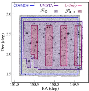
Fig. 1. Layout of the COSMOS field. The image in background is the χ2-stacked zY JHK
simage. The COSMOS 2 deg2field is enclosed
by a blue line, while the UltraVISTA survey is inside the purple con-tour. UltraDeep stripes, where UltraVISTA exposure time is higher, are delimited by magenta lines. A purple (magenta) shaded area shows the Deep (UltraDeep) region actually used in this paper.
down to 0.2, is then discussed in Sect.6. Eventually, we sum-marise our work in Sect.7.
Throughout this paper we assume a flatΛCDM cosmology withΩm= 0.3, ΩΛ= 0.7, and h70≡ H0/(70 km s−1Mpc−1)= 1.
Galaxy stellar masses, when derived from SED fitting, scale as the square of the luminosity distance; therefore, there is a factor h−2
70 kept implicit throughout this paper (see Croton 2013, for
an overview on cosmology conversions and their conventional notation). Magnitudes are in the AB system (Oke 1974).
2. Dataset
A description of our dataset is summarised in Sect.2.1. Sect.2.2
offers a comprehensive discussion about its completeness as a function of flux in IRAC channel 1 (i.e., at ∼ 3.6 µm). Core of our analysis is the COSMOS2015 catalogue, recently published inLaigle et al. (2016, L16 in the following); other COSMOS datasets provide additional information. A complete list of the surveys carried out by the collaboration can be found in the o ffi-cial COSMOS website.1
2.1. Photometry
One cornerstone of the COSMOS2015 photometry comes from the new Y, J, H, and Ks images from the second data release
(DR2) of the UltraVISTA survey (McCracken et al. 2012), along with the z++band from Suprime-Cam at Subaru (Miyazaki et al. 2012). These images were added together to build a stacked detection image, as explained below.
The catalogue also includes the broadband optical filters u∗, B, V, r, i+, and 14 intermediate and narrow bands. In NIR,
UltraVISTA is complemented by the y band images from the Hyper Suprime-Cam (HSC), as well as H and Ksfrom WIRCam
(at the Canada-France-Hawaii Telescope). The point-spread function (PSF) in each band from u∗ to Ks is homogenised, so
that the fraction of flux in a 300 diameter aperture suffers from
band-to-band seeing variations by less than 5% (see Fig. 4 in L16). Space-based facilities provided data in near-UV (from the GALEX satellite,Zamojski et al. 2007) and MIR (from IRAC on board the Spitzer Space Telescope), along with high-resolution optical images (ACS camera on board HST, see Sect. 3.2). Galaxies with an X-ray counterpart from XMM (Brusa et al. 2007) or Chandra (Marchesi et al. 2016) are excluded from the following analysis as their photometric redshifts, or the stellar mass estimates, would be likely corrupted by contamination of their active galactic nuclei (AGN). They represent less than 1% of the whole galaxy sample. The entire photometric baseline of COSMOS2015 is summarised in Table 1 of L16.
Spitzer data represent another pillar of this catalogue, prob-ing the whole COSMOS area at 3.6−8.0 µm, i.e. the wavelength range where the redshifted optical spectrum of z & 3 galaxies is observed. Such a crucial piece of information mainly comes from SPLASH but other surveys are also included, in particular the Spitzer-Cosmic Assembly Near-Infrared Deep Extragalac-tic Legacy Survey (S-CANDELS,Ashby et al. 2015). Further details about how Spitzer/IRAC photometry was extracted and harmonised with the other datasets can be found in L16.
Compared with the previous version of the catalogue (Ilbert et al. 2013) the number of sources doubled because of the longer exposure time of the UltraVISTA DR2 in the so-called “Ultra-Deep” stripes (hereafter indicated with AUD, see Fig. 1). In
that area of 0.62 deg2 we reach a 3σ limiting magnitude (in a
300diameter aperture) Klim,UD = 24.7, while in the remaining
“Deep” area (dubbed AD= 1.08 deg2) the limit is Klim,D= 24.0.
The larger number of detected sources in DR2 is also due to the new χ2 stacked image produced in L16. Image stacking is a panchromatic approach for identification of galaxy sources, pre-sented for the first time inSzalay et al.(1999). With respect to the previous UltraVISTA (DR1) stacking, in L16 we co-add not only NIR images but also the deeper z++ band, using the code SWarp (Bertin et al. 2002). Pixels in the resulting zY JHK image are the weighted mean of the flux in each stacked filter. As a result, the catalogue contains ∼ 6 × 10⁵objects within 1.5 deg2, 190 650 of them in AUD. In L16 we also show the good
agree-ment of colour distributions, number counts, and clustering with other state-of-the-art surveys.
For each entry of the COSMOS2015 catalogue we search for a counterpart in the four Spitzer-IRAC channels using the code IRACLEAN (Hsieh et al. 2012).2 The procedure is
de-tailed in L16. In brief, positional and morphological informa-tion in the zY JHKsdetection image is used as a prior to identify
IRAC sources and recover their total flux. In this latest version, IRACLEAN produces a weighing scheme from the surface bright-ness of the prior, to correctly deblend objects that are near to each other less than ∼ 1 FWHM of the IRAC PSF. For each source a flux error is estimated by means of the residual map, i.e. the IRAC image obtained after subtracting the flux associ-ated to detections.
0
1
2
3
4
5
6
redshift
0
1000
2000
3000
4000
5000
N(z)
CANDELS (N17)
missing in COSMOS2015
22
23
24
25
26
[3.6] mag
0.4
0.5
0.6
0.7
0.8
0.9
1.0
N
m at ch ed/N
to t2.5<z<3.5
3.5<z<4.5
4.5<z<6.0
22
23
24
25
26
[3.6] mag
0.4
0.5
0.6
0.7
0.8
0.9
1.0
N
m at ch ed/N
to tDeep-like limits
2.5<z<3.5
3.5<z<4.5
4.5<z<6.0
Fig. 2. Upper panel: Redshift distribution of the whole CAN-DELS sample in the COSMOS field, taken fromNayyeri et al.(2017, N17, gray filled histogram). We also identify the N17 objects that do not have a counterpart (within 0.800
) in the COSMOS2015 catalogue, showing their N(z) with a red histogram. Middle panel: ratio between the CANDELS objects with a match in COSMOS2015 (Nmatched) and
all the CANDELS entries (Ntot) in bins of [3.6] magnitude (filled
cir-cles). These estimates are divided into three redshift bins in the range 2.5 < zphot,N17< 6 (see colour code in the legend); a dashed line marks
the 70% completeness. Lower panel: Similar to the middle panel, but the Nmatched/Ntotratio is estimated to reproduce the sensitivity depth of
UltraVISTA-Deep.
2.2. Flux limits and sample completeness at high redshift We aim to work with a flux-limited sample to restrict the analysis to a sample sufficiently complete with photometric errors suffi-ciently small. In L16 the completeness as a function of stellar mass has been derived in bins of Ksmagnitudes, but this choice
is not suitable for the present analysis, which extends to z ∼ 6. Up to z ∼ 4, a Ks-band selection is commonly used to derive a
completeness limit in stellar mass (e.g.Ilbert et al. 2013;Muzzin et al. 2013a; Tomczak et al. 2014), but at higher redshifts this filter probes a rest-frame range of the galaxy spectrum particu-larly sensitive to recent star formation. Indeed, the Balmer break moves to wavelengths larger than 2 µm and most of the stellar light coming from K- and M-class stars is observed in the IRAC channels. This makes a [3.6] selection suitable at z > 4. In
2 The wavelength range of the four channels is centred respectively at
3.6, 4.5, 5.8, and 8.0 µm; in the following we refer to them as [3.6], [4.5], [5.8], and [8.0].
this paper we will apply a selection in Ksor [3.6] depending on
the redshift, always choosing the most direct link between stel-lar light and mass. Moreover, we will show in AppendixBthat even between z ∼ 2 and 4, where in principle both bands can be used, a cut in [3.6] is recommended. Thus, for our analysis at 2.5 < z < 6, we will extract from the parent catalogue a sample of galaxies with magnitude [3.6] < [3.6]lim.
Determining [3.6]limis not as straightforward as for the Ks
band. The nominal 3σ depth (equal to 25.5 mag for a 300 di-ameter aperture) has been calculated by means of the rms map of the [3.6] mosaic, after removing detected objects. However our sources were originally found in the co-added image, so the completeness of the final sample depends not only on possible issues in the IRAC photometric extraction (due e.g. to confusion noise) but also in zY JHKs. For instance, we expect to miss red
galaxies with [3.6] 25.5 but too faint to be detected in NIR. Their impact should not be underestimated, given the mount-ing evidence of strong dust extinction in high-z galaxies (e.g.
Casey et al. 2014a;Mancini et al. 2015). This is a limitation in any analysis that uses optical/NIR images as a prior to deblend IR sources (e.g.Ashby et al. 2013,2015). Such an approach is somehow necessary, given the lower resolution of the IRAC camera, but exceptions do exist (e.g.Caputi et al. 2011, where IR photometry is extracted directly from 4.5 µm images without any prior).
To estimate [3.6]lim we make use of the catalogue built
by Nayyeri et al. (2017, hereafter referred as N17) in the 216 arcmin2 of the CANDELS-COSMOS field (Grogin et al. 2011;Koekemoer et al. 2011). Since CANDELS falls entirely in our Ultra-Deep area, N17 can be used to directly constrain [3.6]lim,UD. The authors rely on F160W images (∼ 1.6 µm) from
the HST/WFC3 camera and extract IRAC sources using the soft-ware TFIT (Papovich et al. 2001; Laidler et al. 2007). Their approach is similar to Galametz et al. (2013), who derive the UV-to-IR photometry in another CANDELS field, overlapping with the Ultra-Deep Survey (UDS) of UKIDSS. The 5σ limit-ing magnitude in the F160W band is 26.5, while the data from Spitzer are the same as in L16. Then, we can test the effects of a different extraction algorithm and sensitivity depth of the prior.
First, we match galaxies from COSMOS2015 and N17 (within a searching radius of 0.800) and compare their
pho-tometric redshift estimates and [3.6] magnitudes to check for possible bias. We confirm the absence of significant offsets ([3.6]L16− [3.6]N17< 0.03 mag) as previously verified by Stein-hardt et al.(2014). The [3.6] number counts of COSMOS2015 are in excellent agreement with CANDELS, for magnitudes . 24.5; after restricting the comparison inside the AUDregion,
counts agree with < 20% difference until reaching [3.6] = 25, where the number of UltraDeep sources starts to decline com-pared to CANDELS. Despite such a small fraction of missing sources, our z & 3 statistical analysis would nonetheless suf-fer from severe incompleteness if most of them turned out to be at high redshift. For this reason, we inspect the zphot
distri-bution of 11 761 galaxies (out of 38 671) in N17 not matching any COSMOS2015 entry. They are extremely faint objects with F160W & 26, most of them without a counterpart even in our IRAC residual maps (see below).
The CANDELS photometric redshifts (zphot,N17) have been
computed independently by several authors, by means of di ffer-ent codes (seeDahlen et al. 2013). Here we use the median of those estimates, which is generally in good agreement with our zphotfor the objects in common. The upper panel of Fig.2shows
that galaxies excluded from the CANDELS-COSMOS matching have a redshift distribution N(z) similar to the whole N17
sam-ple. Restricting the analysis to 2.5 < zphot,N17 6 3.5 galaxies,
we clearly see that the fraction of N17 galaxies not detected in COSMOS2015 increases towards fainter magnitudes. The same trend, despite a larger shot noise due to the small-number statis-tics, is visible at higher redshifts. Taking CANDELS as a ref-erence “parent sample”, the fraction of sources we recover is a proxy of the global completeness of COSMOS2015. As shown in Fig.2(middle panel) we can assume [3.6]lim,UD= 25 as a
reli-able > 70% completeness limit for our AUDsample up to z= 6.
We can also evaluate such a limit in AD([3.6]lim,D) although
that region does not overlap CANDELS. We repeat the proce-dure described above after applying a cut in z+, Y, J, H, and Ks
bands of N17, corresponding to the 3σ limiting magnitudes in the AD area. The resulting threshold is almost 1 mag brighter
than [3.6]lim,UD, with a large scatter at zphot,N17 > 3.5 (Fig.2,
bottom panel). However, we warn that such a “mimicked” se-lection is just an approximation, less efficient than the actual ADextraction.3 With this caveat in mind, we suggest to assume
[3.6]lim,D= 24 up to z ∼ 4. However, the analysis in the present
paper is restricted to the AUDsample and an accurate evaluation
of [3.6]lim,Dis beyond our goals.
In addition, we run SExtractor (Bertin & Arnouts 1996) on the [3.6] and [4.5] residual maps to check whether the recovered sources coincide with those in CANDELS. Most of the latter ones are not found in the residual maps, because they are fainter than the SPLASH background noise (& 25.5 mag), with a low signal-to-noise ratio (S /N < 2) that prevents us to effectively identify them with SExtractor. For the 20% CANDELS un-matched objects that are brighter than [3.6]lim,UD, their absence
in the residual maps can be explained by blending effects: if a MIR source does not correspond to any COSMOS2015 de-tection, IRACLEAN may associate its flux to a nearby extended object. This highlights the capability of HST/WFC3 to correct for IRAC source confusion better than our ground-based im-ages, although the deeper sensitivity we shall reach with the on-coming VISTA and HSC observations should dramatically re-duce the gap.4 Eventually, we visually inspect 22 sources at
24 < [3.6] < 25 recovered from the IRAC residual map but not found in the N17 sample. These objects are not resolved in the F160W image, neither in UltraVISTA. They appear also in the IRAC [4.5] residual map suggesting that they should not be artefacts, rather a peculiar type of 3 < z < 5 galaxies with a prominent D4000 break (or less probably, z ∼ 12 galaxies) that we shall investigate in a future work.
3. Photometric redshift and galaxy classification
We estimate the zphot of COSMOS2015 sources by fitting
synthetic spectral energy distributions (SEDs) to their multi-wavelength photometry. The COSMOS2015 catalogue already
3 The Subaru z+band available in N17 is similar to z++, albeit
shal-lower; Y, J, H, Ks photometry is taken from UltraVISTA DR1 and
therefore its depth is comparable to our Deep sample. We restrict the N17 sample to be “Deep-like” by simply considering as detected ob-jects whose flux is above the sensitivity limits in at least one of these five bands. We stress that such an approach differs from the actual AD
also because doing this approximation we did not take into account the correction related to PSF homogenisation.
4 As a consequence of this blending issue, the IRAC flux of some
of our bright galaxies (and stars) is expected to be overestimated, but less than 40% since the secondary blended source is generally > 1 mag fainter. Some of the CANDELS unmatched objects may also be cor-rupted detections, since for this test we did not apply any pre-selection using SExtractor quality flags.
provides photometric redshifts and other physical quantities (e.g., galaxy stellar masses) derived through an SED fitting pro-cedure detailed in L16. Here we follow the same approach, us-ing the code LePhare (Arnouts et al. 2002;Ilbert et al. 2006) but with a configuration optimised for high-z galaxies (Sect.3.1).
The main reasons for a new SED fitting computation at z > 2.5 are the following:
– L16 explored the parameter space between z= 0 and 6, but to build an accurate PDF(z) for galaxies close to that upper limit one has to enlarge the redshift range. Therefore, we scan now a grid z= [0, 8] to select galaxies between zphot= 2.5 and 6.
– We have improved the method for removing stellar interlop-ers, which is now based on a combination of different star vs galaxy classifications, with particular attention to low-mass stars (see Sect.3.2).
– With respect to L16, we included in the library additional high-z templates, i.e. SEDs of extremely active galaxies with rising star formation history (SFH) and highly attenuated galaxies with E(B − V) > 0.5.
Our results will replace the original photometric redshifts of L16 only at z > 2.5 (Sect.3.3). Galaxies with a new zphot < 2.5 are
not considered, so below z = 2.5 the sample is the same as in L16. In any case, the variation at low z is negligible, given the high percentage of galaxies that preserve their original redshift. A comparison between the original L16 SED fitting and our new results can be found in AppendixA.
3.1. Photometric redshift of z> 2.5 galaxies
We fit the multi-band photometry of the entire catalogue and then select galaxies with zphot> 2.5. We apply zero-point offsets in all
the bands as prescribed in L16. Also when S /N < 1, we consider the flux measured in that filter (and its uncertainty) without re-placing it with an upper limit. This choice allows us to take into account non-detections without modifying the way in which the likelihood function is computed (whereas a different implemen-tation is required to use upper limits, seeSawicki 2012).
Our SED fitting library includes early- and late-type galaxy templates fromPolletta et al.(2007), together with 14 SEDs of star-forming galaxies from GALAXEV (Bruzual & Charlot 2003, see also Sect.4.1). With this code we also produce templates of passive galaxies at 22 different ages (from 0.5 to 13 Gyr). These are the same templates used in L16. In addition, as mentioned above, we use two GALAXEV templates that represent starburst galaxies with an increasing SFH (Behroozi et al. 2013;da Cunha et al. 2015; Sparre et al. 2015). The age of both templates is 100 Myr. Instead of using an exponentially increasing SFH (Maraston et al. 2010) we opt for a multi-component parametri-sation (Stark et al. 2014): a constant SFH is superimposed to a delayed τ model with SFR ∝ τ−2te−t/τ(seeSimha et al. 2014)
where the e-folding time τ is equal to 0.5 Gyr and t= 10−40 Myr (Papovich et al. 2001,2011;Smit et al. 2014).
We add to each synthetic SED the principal nebular emission lines: Lyα λ1216, [OII] λ3727, Hβ λ4861, [OIII]λλ 4959, 5007, Hα λ6563. We calibrate the lines starting from the UV-[OII] re-lation ofKennicutt(1998), but we let the [OII] equivalent width vary by ±50% with respect to what the equation prescribes. The approach is fully empirical, with line strength ratios based on
Anders & Alvensleben(2003) andMoustakas et al.(2006). The addition of nebular emission lines has been discussed in several studies (see Sect.5.2). In general, it is considered as an improve-ment: e.g.Ilbert et al.(2009), by including templates with emis-sion lines, increase the zphot accuracy by a factor ∼ 2.5. Such
Fig. 3. Colour-colour diagrams for removing stellar contaminants. Only spectroscopic measurements with quality flags 3 or 4 (CL > 95%) are shown in the figure. Upper panel: (B−z++) vs (z++−[3.6]). Galaxies detected in the B band are shown with filled circles coloured from red to yellow according to their zspec. Lower panel: (H − Ks) vs (Ks− [4.5]).
Circles with red-to-yellow colours are B drop-outs, while grey circles are the remaining spectroscopic galaxies at z. 3. In both panels, solid lines delimit the conservative boundaries we chose for the stellar locus. These are described by the following equations: (z++− [3.6]) < 0.5(B − z++) − 1 in the upper panel, and (Ks− [3.6]) < (H − Ks) ∧ (H − Ks) < 0.03
in the lower panel. Stars spectroscopically confirmed are plotted with cyan symbols. Typical photometric errors are. 0.05 mag for object with [3.6] < 24, and increase up to 0.08−0.12 mag for fainter ones.
a gain is due to the fact that strong optical lines (like [OII] or Hβ-[OIII]) can boost the measured flux and alter galaxy colours (e.g.Labbé et al. 2013).
We assume for nebular emission the same dust attenuation as for stars (seeReddy et al. 2010;Kashino et al. 2013) although the issue is still debated (Förster Schreiber et al. 2009;Wuyts et al. 2013). Moreover, we do not implement any specific prior to con-trol the level of emission line fluxes, although recent studies in-dicate that their equivalent width (EW) and strength ratio evolve with redshift (e.g.Khostovan et al. 2016; Faisst et al. 2016a). Nevertheless, a stronger bias in the computation is produced by neglecting these lines, rather than by their rough modelling (see
González et al. 2011;Stark et al. 2013;Wilkins et al. 2013). Attenuation by dust is implemented in the SED fitting choos-ing among the followchoos-ing extinction laws: Prévot et al. (1984, SMC-like),Calzetti et al.(2000), and two modified versions of Calzetti’s law that include the characteristic absorbing feature at 2175 Å (the so-called “graphite bump”,Fitzpatrick & Massa 1986) with different strength. The optical depth is free to vary from E(B − V)= 0 to 0.8, to take into account massive and heav-ily obscured galaxies at z > 3 (up to AV ' 3, e.g.Spitler et al. 2014).
Our initial sample at 2.5 < z 6 6 includes 92 559 galax-ies. The photometric redshift assigned to each of them is the median of the probability distribution function (PDF) obtained after scanning the whole template library. Hereafter, for sake of simplicity, for the reduced chi squared of a fit (often referred as χ2red) we will use the short notation χ2.5 The zphoterror (σz)
corresponds to the redshift interval around the median that de-limits 68% of the integrated PDF area. The same definition of 1σ error is adopted for stellar mass estimates as well as SFR, age, and rest-frame colours (see Sect.4). As an exception, we prefer to use the best-fit redshift when the PDF(z) is excessively broad or spiky (i.e. there are a few peaks with similar likeli-hood) and the location of the median is thus highly uncertain; we identify 2 442 galaxy in this peculiar condition, such that |zmedian− zbest|> 0.3(1 + zbest).
To secure our zphot> 2.5 sample, we apply additional
selec-tion criteria. In the redshift range of u-to-V drop-outs (zphot &
3.2) we require galaxies not to be detected in those optical bands centred at < 912(1+ zphot) Å. This condition is naturally
satis-fied by 97.3% of the sample. We also remove 249 sources with χ2> 10. We prefer not to implement criteria based on visual
in-spection of the high-z candidates, to avoid subjective selections difficult to control.
3.2. Stellar contamination
To remove stars from the zphot > 2.5 sample we adopt an
ap-proach similar to Moutard et al. (2016a), combining multiple selection criteria. First, we fit the multi-wavelength baseline with stellar spectra taken from different models and observa-tions (Bixler et al. 1991;Pickles & J. 1998;Chabrier et al. 2000;
Baraffe et al. 2015). We emphasise that the library contains a large number of low-mass stars of spectral classes from M to T, mainly fromBaraffe et al.(2015). Unlike dwarf star spectra used in previous work (e.g.Ouchi et al. 2009;Bouwens et al. 2011;
Bowler et al. 2014) those derived fromBaraffe et al.(2015) ex-tend to λr.f. > 2.5 µm and therefore SPLASH photometry
con-tributes to disentangle their degeneracy with distant galaxies (Wilkins et al. 2014).
We compare the χ2 of stellar and galaxy fits, and flag an
object as star if χ2gal −χ2star > 1. When the χ2 difference is smaller than this confidence threshold we use additional indi-cators, namely (i) the stellar locus in colour-colour diagrams and (ii) the maximum surface brightness (µmax) above the local
back-ground level. For objects with 0 < χ2 gal−χ
2
star 6 1 we also set
zphot= 0 when the criteria (i) or (ii) indicates that the source is a
star.
The diagrams adopted for the diagnostic (i) are (z++− [3.6]) vs (B − z++) and (H − Ks) vs (K − [3.6]); the former is analogous
of the BzK byDaddi et al.(2004), the latter has been used e.g. in
Caputi et al. (2015). The two diagrams are devised using the predicted colours of both stars and galaxy models, and tested by means of the zspecsample (Fig.3). The latter is used for
galax-ies not detected in the B band (mainly drop-outs at z & 4) for which the (z++− [3.6]) vs (B − z++) diagnostic breaks down (see L16, Fig. 15). In each colour-colour space we trace a conserva-tive boundary for the stellar locus, since photometric uncertain-ties increase the dispersion in the diagram and stars can be scat-tered out from the original sequence. Method (ii) is detailed in
5 That is χ2≡χ2
o/(Nfilt− NDOF), where χ2ois the original definition of
goodness of fit, based on the comparison between the fluxes observed in Nfiltfilters and those predicted by the template (NDOFbeing the degrees
of freedom in the fitting, see definitions e.g. inBolzonella et al. 2000).
Fig. 4. Comparison between zspecand zphot, for spectroscopic
galax-ies (and stars) with [3.6] < 25 (empty circles). Only robust spectro-scopic measurements (CL > 95%) are plotted, and coloured according to their survey: zCOSMOS faint (Lilly et al., in preparation), VUDS (Le Fèvre et al. 2015), FMOS-COSMOS (Silverman et al. 2015), a survey with the FORS2 spectrograph at VLT (Comparat et al. 2015), a survey with DEIMOS at Keck II (Capak et al., in preparation), and grism spec-troscopy from HST/WFC3 (Krogager et al. 2014). In the background we also show the comparison between zspecand the original photometric
redshifts of L16 (grey crosses). Upper panel: In addition to zphotvs zspec,
in the bottom-left corner we report the number of objects considered in this test (Ngal), the σzerror defined as the NMAD, and the fraction of
catastrophic outliers (η). The dashed line is the zphot = zspecreference.
Lower panel: Scatter of the zphot− zspecvalues, with the same colour
code as in the upper panel. Horizontal lines mark differences (weighed by 1+ zspec) equal to ±0.05 (dotted lines) or null (dashed line).
Leauthaud et al.(2007) andMoutard et al.(2016b). The surface brightness measurements in the wide I-filter of HST (F814W) come from the Advanced Camera for Surveys (ACS) images analysed byLeauthaud et al.(2007). Stars are segregated in the µmax-I plane, which has been shown to be reliable at I. 25.6
3.3. Validation through spectroscopy and self-organizing map
We use a catalogue of almost 100 000 spectroscopic redshifts to quantify the uncertainties of our zphotestimates. These data were
obtained during several campaigns, with different instruments and observing strategies (for a summary, see Table 4 of L16). They have been collected and harmonised in a single catalogue by Salvato et al. (in preparation). Such a wealth of spectroscopic information represents an unequalled benefit of the COSMOS field.
The zspecmeasurements used as a reference are those with
the highest reliability, i.e. a confidence level (CL) > 95% (equal to a selection of quality flags 3 and 4 according to the scheme introduced byLe Fèvre et al. 2005). We limit the comparison to sources brighter than [3.6]= 25, ignoring secure low-z galaxies (those having both zspec and zphot below 2.5). Eventually, our
test sample contains 1 456 objects. The size of this sample is
6 Leauthaud et al.also discuss the limitations of the “stellarity index”,
another commonly used classification provided by SExtractor. This indicator is less accurate than the one based on µmax, especially for faint
compact galaxies (seeLeauthaud et al. 2007, Fig. 4). We then decided not to add stellarity indexes to our set of criteria.
0 20 40 60 D1 0 20 40 60 80 100 120 140 D2 0 1 2 3 4 5 6
Median spec-z (quality flags 3 and 4)
0 20 40 60 D1 0 20 40 60 80 100 120 140 D2 0 1 2 3 4 5 6
Median photo-z (stars and galaxies with z>2.5)
Fig. 5. The bi-dimensional self-organising map of the COSMOS2015 catalogue (the two folded dimensions have generic labels D1and D2). In
the left panel, only robust spectroscopic objects (CL > 95%) are shown. In the right panel, the SOM is filled with photometric objects (stars and zphot> 2.5 galaxies). In both cases, each cell of the map is colour-coded according to the median redshift of the objects inside the cell (empty cells
are grey, cells filled by stars are black).
unique: with 350 galaxies at zspec> 3.5, it is more than twice the
number of robust spectroscopic redshifts available in CANDELS GOODS-South and UDS, used inGrazian et al.(2015).
Among the 301 spectroscopic stars considered, > 90% of them are correctly recovered by our method, with only three stel-lar interlopers with zphot > 2.5. On the other hand, less than
1% of the spectroscopic galaxies are misclassified as stars. The catastrophic error rate is η = 12%, considering as an outlier any object with |zphot− zspec| > 0.15(1 + zspec). The precision
of our photometric redshifts is σz= 0.03(1 + z), according to the
normalised median absolute deviation (NMAD, Hoaglin et al. 1983) defined as 1.48 × median{|zphot− zspec|/(1 + zspec)}. These
results (Fig.4) summarise the improvement with respect to the photometric redshifts of L16: we reduce the number of catas-trophic errors by ∼ 20%, and we also observe a smaller bias at 2.5 < z < 3.5 (cf. Fig. 11 of L16).
The comparison between zspecand zphotis meaningful only
if the spectroscopic sample is an unbiased representation of the “parent” photometric sample. Otherwise, we would test the re-liability of a subcategory of galaxies only. We introduce a self-organizing map (SOM,Kohonen 1982) to show that our spectro-scopic catalogue provides a representative sample of the under-lying colour and redshift distribution. The algorithm version we use, specifically implemented for astronomical purposes, is the one devised inMasters et al.(2015). The SOM allows to reduce a high-dimensional dataset in a bi-dimensional grid, without los-ing essential topological information. In our case, the startlos-ing manifold is the panchromatic space (fifteen colours) resulting
from the COSMOS2015 broad bands: (NUV − u), (u − B), ..., ([4.5] − [5.8]), ([5.8] − [8.0]). As an aside, we note that the SOM dimensions do not necessarily have to be colours: in prin-ciple the parameter space can be enlarged by including other properties like galaxy size or morphological parameters. Each coloured cell in the map (Fig.5) corresponds to a point in the 15-dimensional space that is non-negligibly occupied by galax-ies or stars from the survey. Since the topology is preserved, objects with very similar SEDs – close to each other in the high-dimensional space – will be linked to the same cell (or to adja-cent cells).
We inspect the distribution of spectroscopic objects in the SOM, using them as a training sample to identify the region of high-z galaxies (Fig.5, left panel). The COSMOS spectroscopic catalogue samples well the portion of parameter space we are interested in, except for the top-left corner of the map where we expect, according to models, the bulk of low-mass stars. The lack of spectroscopic measurements in that region may affect the precise evaluation of the zphot contaminant fraction. Other
cells that are weakly constrained correspond to the SED of star-forming galaxies with i & 23 mag and z < 2 (Masters et al. 2015), which however are not pivotal for testing our estimates.
After the spectroscopic calibration, we insert zphot > 2.5
galaxies in the SOM along with photometric stars (Fig.5, right panel). Given the larger size of the photometric catalogue, cells occupation is more continuous and extended (see e.g. the stellar region in the bottom-right corner). By comparing the two panels of Fig.5, one can see that the zphot > 2.5 galaxies are
concen-23
24
25
26
27
[3
.
6] mag
9.0
9.5
10.0
10.5
11.0
lo
g(
M/
M ¯)
3.0<z<3.5 3.5<z<4.5 4.5<z<5.50.0 0.5 1.0
f
obs=
N
([3
.
6]
<
25)
/N
totFig. 6. Stellar mass completeness as a function of redshift. Blue circles, green squares, red triangles represent CANDELS galaxies at 2.5 < zphot,N17 6 3.5, 3.5 < zphot,N176 4.5, 4.5 < zphot,N176 6
respec-tively. The cut in apparent magnitude of our sample ([3.6]lim) is marked
with a vertical dashed line. Slant dotted lines show a conservative es-timate of the stellar mass limit, corresponding to the M/L ratio of an old SSP with AV = 2 mag. Three crosses in the bottom-right corner of
the main panel show the average x- and y-axis uncertainties in the cor-responding bin of redshift. The histograms on the right (same colours and z-bins of the scattered points) show the ratio of N17 galaxies with [3.6] < [3.6]limover the total N17 sample. This fraction is named fobs
since they are the objects that would be observed within the magnitude limit of COSMOS2015. Below each histogram, an arrow indicates the stellar mass threshold Mlim(see Sect.4.2).
trated in the SOM region that has been identified as high-z by the spectroscopic training sample. Although the latter is more sparse, about 60% of the area covered by zphot > 2.5 galaxies is
also sampled by spectroscopic measurements, which are quan-titatively in good agreement: in 82% of those cells that contain both photometric and spectroscopic redshifts, the median of the former ones is within 1σz from the median of the zspec objects
laying in the same cell. Moreover, by plotting individual galax-ies (not shown in the Figure) one can verify that catastrophic zphot
errors are randomly spread across the SOM, not biasing any spe-cific class of galaxies.
4. Stellar mass estimate and completeness
After building a zphot > 2.5 galaxy sample, we run LePhare to
estimate their stellar mass, star formation rate (SFR), and other physical parameters such as rest frame colours. This is described in Sect.4.1, while in Sect.4.2we compute stellar mass com-pleteness limits and we argue in favour of a [3.6] selection to work with a mass-complete sample up to z ∼ 6 (see also Ap-pendixB). By means of their rest-frame colours we then identify reliable quiescent galaxies (Sect.4.3).
4.1. Galaxy stellar mass
We estimate stellar mass and other physical properties of the COSMOS2015 galaxies always at fixed z ≡ zphot. We fit their
multi-wavelength photometry with a library of SEDs built us-ing the stellar population synthesis model ofBruzual & Charlot
(2003, hereafter BC03). The M estimates are the median of the PDF marginalised over the other parameters. This kind of
esti-mate is in good agreement with the stellar mass derived from the PDF peak (i.e., the best-fit template). The difference between median and best-fit values is on average 0.02 dex, with a rms of 0.11 dex.
The galaxy templates given in input to LePhare are con-structed by combining BC03 simple stellar populations (SSPs) according to a given star formation history (SFH). Each SSP has an initial mass function (IMF) that followsChabrier(2003), while the stellar metallicity can be Z = 0.02, 0.008, or 0.004.7
These stellar metallicities have been chosen to encompass the range observed up to z ∼ 4−5 (e.g.Maiolino et al. 2008; Som-mariva et al. 2012); they are also in agreement with hydrodynam-ical simulations (Ma et al. 2016). For each template we combine SSPs with the same metallicity (i.e. there is no chemical enrich-ment in the galaxy model, nor interpolation between the three given Z values).
We assumed various SFHs, namely “exponentially declin-ing” and “delayed declindeclin-ing”. The former ones have SFR(t) ∝ e−t/τ, while the shape of the latter is ∝ te−t/τ. For the exponen-tially declining profiles, the e-folding time ranges from τ= 0.1 to 30 Gyr, while for delayed SFHs the τ parameter, which also marks the peak of SFR, is equal to 1 or 3 Gyr. We post-process the BC03 templates obtained in this way by adding nebular emis-sion lines as described in Sect.3.1. Dust extinction is imple-mented assuming 0 6 E(B − V) 6 0.8. We allow for only one attenuation law, i.e.Calzetti et al.(2000) with the addition of the 2175 Å feature (seeScoville et al. 2015).
We have tried a few alternate configurations to quantify the amplitude of possible systematics (see Sect.5.2for a detailed discussion). We added for example a second attenuation curve with slope proportional to λ−0.9 (Arnouts et al. 2013). Such a choice increases the number of degenerate best-fit solutions without introducing any significant bias: Calzetti’s law is still preferred (in terms of χ2) by most of the objects at z& 3. Other
modifications, e.g. the expansion of the metallicity grid, have a larger impact, as also found in other studies (e.g.Mitchell et al. 2013). Simplifying assumptions are somehow unavoidable in the SED fitting, not only for computational reasons but also be-cause the available information (i.e., the multi-wavelength base-line) cannot constrain the parameter space beyond a certain num-ber of degrees of freedom. This translates into systematic offsets when comparing different SED fitting recipes. The impact of these systematics on the SMF is clearly visible inConselice et al.
(2016, Fig. 1), where the authors overplot a wide collection of measurements from the literature: already at z < 1, where data are more precise, the various SMF estimates can differ even by a factor ∼ 3. We emphasise that one advantage of our work, whose goal is to connect the SMFs at different epochs, is to be less af-fected by SED fitting uncertainties than analyses that combine measurements from different papers. In our case, SED fitting systematics (unless they have a strong redshift or galaxy-type de-pendence) will cancel out in the differential quantities we want to derive.
As mentioned above, the 68% of the integrated PDF(M) area gives an error to each stellar mass estimate. However, the PDF is obtained from χ2-fit templates at fixed redshift. To compute
stel-lar mass errors (σm) including the additional uncertainty
inher-ited from σz, we proceed in a way similar toIlbert et al.(2013).
They generate a mock galaxy catalogue by perturbing the origi-nal photometry and redshifts, proportioorigi-nally to their errors.
Af-7 We avoid to use Z
units since recent work suggests that solar
metal-licity is lower than the “canonical” value of 0.02 (e.g., Z = 0.0134 in
ter recomputing the stellar mass of each galaxy, the authors de-fine its uncertainty as the difference between new M and the original estimate, namely∆Mi ≡ log(MMC,i/Mi) (for the i-th
galaxy).
We implement a few modifications with respect toIlbert et al.
(2013). Instead of adding noise to photometry and zphot, we
ex-ploited the PDFs. Moreover, we produce 100 mock catalogues, instead of a single one. We perform a Monte Carlo simulation, re-extracting 100 times the zphotof each galaxy, accordingly to
its PDF(z). Each time, we run again LePhare with the redshift fixed at the new value (zMC) to compute the galaxy stellar mass
MMC and the offset from the original value. We group galaxies in bins of redshift and mass to obtain an estimate of σmfrom the
distribution of their∆M. As inIlbert et al.(2013), this is well fit by a Gaussian multiplied by a Lorentzian distribution:
D(M0, z) = 1 σ√2π exp −M2 0 2σ2 × τ 2πh(τ2)2+ M2 0 i , (1)
where M0 is the centre of the considered stellar mass bin. The
parameters σ and τ are in principle functions of M0 and z, left
implicit in Eq. 1 for sake of clarity. We find σ ' 0.35 dex, without a strong dependence on M and neither on z, at least for 9.5 < log(M/M ) < 11.5. Also τ does not depend significantly
on stellar mass but it increases as a function of redshift. The re-lation assumed inIlbert et al.(2013), namely τ(z)= 0.04(1 + z), is still valid for our sample. We note that the value of σ is in-stead smaller (it was 0.5 dex inIlbert et al. 2013), reflecting the increased quality of the new data. At face value, one can as-sume σm(M)= 0.35 dex (neglecting the Lorentzian “wings” of
D); however a careful treatment of stellar mass uncertainties re-quires to take into account the whole Eq. (1). This computation gives us an idea about the impact of σz on the stellar mass
es-timate: the errors resulting from the PDF(M), after fixing the redshift, are usually much smaller (e.g. < 0.3 dex for 90% of the galaxies at 3.5 < z 6 4.5). Further details about the impact of σmon the SMF are provided in Sect.5.5.
4.2. Stellar mass limited sample
To estimate the stellar mass completeness (Mlim) as a function
of redshift, we apply the technique introduced byPozzetti et al.
(2010). In each z-bin, a set of “boundary masses” (Mresc) is
ob-tained by taking the most used best-fit templates (those with the minimum χ2for 90% of the galaxies in the z-bin) and rescaling
them to the magnitude limit: log Mresc = log M + 0.4([3.6] −
[3.6]lim,UD). Then, Mlimis defined as the 90th percentile of the
Mrescdistribution. Taking into account also the incompleteness due to the [3.6] detection strategy (see Fig.2), we expect that in the lowest stellar mass bins of our SMF (at M > Mlim) there
could be a sample incompleteness of 30% at most, caused by objects previously excluded from the IRAC-selection (i.e., with [3.6] > [3.6]lim,UD). Eventually we interpolate the Mlimvalues
found in different z-bins to describe the evolution of the limiting mass: Mlim(z)= 6.3 × 10⁷(1+ z)2.7M .
To verify our calculation, we consider the M vs [3.6] dis-tribution of CANDELS-COSMOS galaxies (N17, see Sect.2.2) after recomputing their stellar mass with LePhare to be consis-tent with our catalogue. By using these deeper data, we verify that the Mlimvalues we found correspond to a completeness of
70−80% (Fig.6). By means of the N17 sample, we can account for stellar mass incompleteness below Mlim (cf.Fontana et al. 2004). The factor we need for such a correction in the low-mass
0.0 0.2 0.4 0.6 0.8 1.0 1.2 1.4 1.6
r
−J
1
2
3
4
5
N
U
V
−r
1 10 102number of objects
Fig. 7. The NUVrJ diagram of galaxies between z= 2.5 and 6 (with their density distribution colour coded in grey shades). The red solid line divides active and passive regions (see Eq.2), while red dashed lines are shifted by ±0.5 mag from that border, to give a rough estimate of the width of the green valley, i.e. the separation between active and passive clumps. The red (blue) cross in the top-left (bottom-right) cor-ner shows the typical uncertainties σNUV−rand σr− jof passive (active)
galaxies at 3 < z <6 4. We also compare our fiducial estimates (based on the nearest observed filter) with colours directly derived from the template SEDs: a solid contour encloses 90% of the former distribu-tion, while a dashed line represents the 90% envelope for the latter.
regime is fobs(z, M), i.e. the fraction of objects at a given
red-shift and stellar mass that are brighter than [3.6]lim,UD. This is
obtained by fitting the histograms shown in Fig. 6(right-hand panel). In doing so we assume that the CANDELS sub-field, which is ∼ 10% of AUD, is large enough to represent the parent
COSMOS2015 volume and sufficiently deeper to probe the full M/L range. The function fobs(z, M) can be used to correct the
SMF of COSMOS2015 at M < Mlim, where the 1/Vmaxweights
start to be biased (see Sect.5).
We also include in Fig.6a comparison between our method and a more conservative one, based on the maximum M/L phys-ically allowed at a given flux limit and cosmic time (see e.g.
Pérez-González et al. 2008). The SED used to this purpose is the one of a galaxy that formed stars in a single initial burst at z= 20, and passively evolves until the desired redshift. Substan-tial extinction (AV = 2 mag) is added to further enlarge M/L.
However, in our redshift range, the statistical relevance of such an extreme galaxy type is small, as one infers from the few CAN-DELS objects sparse in the upper-left corner of Fig.6(see also the discussion inMarchesini et al. 2009, Appendix C). With the maximal M/L ratio we would overestimate the stellar mass com-pleteness threshold by at least a factor 5.
At redshifts between 2.5 and 4 we could in principle evaluate Mlimalso as a function of Ks, with the same empirical approach
used above. The cut to be used in this case is Ks < 24.7 (see
Fig. 16 of L16). However, the Mlimresulting from the Ks-band
selection is 0.2−0.4 dex higher (depending on the redshift) than the threshold derived using the [3.6] band. Such an offset reflects a real difference in the stellar mass distribution of the Ks-selected
sample with respect to the [3.6]-selected one. The latter is an-chored to a χ2-stacked image that includes bands deeper than
Ks, so that the sample is unbiased down to lower masses (more
4.3. Quiescent galaxies classification
We also aim to derive the SMF of passive and active galaxies separately. As shown in the following, the quality of our dataset allows us to extend the classification up to z = 4. Galaxies that stopped their star formation occupy a specific region in the colour-colour diagrams (U − V) vs (V − J), (NUV − r) vs (r − K), or (NUV − r) vs (r − J), as shown in previous work (Williams et al. 2009;Arnouts et al. 2013;Ilbert et al. 2013, respectively). We adopted the last one, dubbed hereafter NUVrJ. Compared to (U − V) vs (V − J), which is often referred as UV J, the use of (NUV − r) makes NUVrJ more sensitive to recent star forma-tion (on 106−108yr scalesSalim et al. 2005;Arnouts et al. 2007).
This property results in a better distinction between fully quies-cent galaxies (sSFR < 10−11yr−1) and those with residual star formation (typically with sSFR ' 10−10yr−1). With UV J, these
two kinds of galaxies occupy the same place in the diagram, as we verified using BC03 models. On the contrary, galaxies with negligible “frostings” of star formation are correctly classified as passive in the NUVrJ.
The NUVrJ indicator is similar to (NUV −r) vs (r − K), with the advantage that at high redshifts the absolute magnitude MJ
is more robust than MK, since for the latter the k-correction is
generally more uncertain. LePhare calculates the absolute mag-nitude at a given wavelength (λr.f.) by starting from the apparent
magnitude in the band closest to λr.f.(1+z). For example at z = 3
the nearest observed filter to compute MJis [4.5], whereas MK
falls beyond the MIR window of the four IRAC channels. The NUVrJ diagram is shown in Fig.7. The density map of our zphot> 2.5 sample highlights the “blue cloud” of star forming
galaxies as well as an early “red sequence”. We also show in the Figure how the NUVrJ distribution changes when colours are derived directly from the template SEDs, without using the nearest observed filter as a proxy of the absolute magnitude. This alternative method is commonly used in the literature, so it is worth showing the different galaxy classification that it yields. The distribution from pure template colours is much narrower (cf. solid and dashed lines in Fig.7) but potentially biased: the SED library spans a limited range of slopes (colours), whereas the nearest filter method – by taking into account the observed flux – naturally includes a larger variety of SFHs.
The boundary of the passive locus is
(NUV − r) > 3(r − J)+ 1 and (NUV − r) > 3.1, (2) defined empirically according to the bimodality of the 2-dimensional galaxy distribution (Ilbert et al. 2013). This border is also physically justified: the slant line resulting from Eq. (2) runs perpendicular to the direction of increasing specific SFR (sSFR ≡ SFR/M). On the other hand, dust absorption moves galaxies parallel to the border, effectively breaking the degener-acy between genuine quiescent and dusty star-forming galaxies. Same properties are observed in (NUV −r) vs (r − K) and (U −V) vs (V − J), as demonstrated e.g. inArnouts et al.(2013) and For-rest et al.(2016).
Rest-frame colour selections have been successfully used up to z ∼ 3 (e.g.Ilbert et al. 2013;Moutard et al. 2016a;Ownsworth et al. 2016). The reliability of this technique at z > 3 has been re-cently called into question bySchreiber et al.(2017): they warn that the IRAC photometry in the COSMOS field could be too shallow to derive robust rest-frame optical colours for galaxies at those redshifts. In order to take into account such uncertainties, our algorithm rejects a filter if its error is larger than 0.3 mag. Most importantly, we evaluate (NUV − r) and (r − J) uncertain-ties, to quantify the accuracy of our NUVrJ selection. For each
galaxy, a given rest-frame colour error (σcolour) is derived from
the marginalised PDF, by considering 68% of the area around the median (similarly to σz). In such a process, the main
contri-butions to σcolorare the photometric uncertainties and the model
k-correction. At 3 < z6 4, the mean errors are σNUV−r = 0.13
and σr−J = 0.10 for the active sample, while σNUV−r= 0.34 and
σr−J = 0.17 for objects in the passive locus (see Fig.7). These
values confirm that our classification is reliable up to z = 4: even the relatively large (NUV − r) uncertainty does not affect it, given the scale of the y axis in Fig.7. Despite the larger uncer-tainties, we also apply the NUVrJ classification at z > 4, iden-tifying 13 potential passive galaxies (4 of them at zphot > 4.5).
In that redshift range, a strong Hα line can contaminate the [3.6] band (which is used to estimate Mr). Comparing their observed
([3.6] − [4.5]) colour with BC03 models (as done inFaisst et al. 2016a) we find that 6 passive candidates at z > 4 could have non-negligible Hα emission (EW= 100−500 Å) while for the others their ([3.6] − [4.5]) is compatible with EW < 50 Å. Nonetheless these z > 4 galaxies need deeper data to be confirmed as passive. Galaxies close to the border defined by Eq. (2) may be mis-classified, but the fraction of objects in that intermediate corri-dor (encompassed by dashed lines in Fig. 7) is small and the bulk of the passive sample should not be significantly contami-nated. We emphasise that by using (NUV − r) instead of (U − V) the larger dynamical scale on the y axis reduces drastically the contamination at the edge of the passive locus. Inside that inter-mediate region galaxies are expected to be in transition from the blue cloud to the red sequence (Moutard et al. 2016a). There-fore, their classification within the active vs passive scheme is not straightforward even from a physical point of view. We will come back to discussing green valley galaxies in Sect.5.4.
5. Results
5.1. Galaxy stellar mass function at z> 2.5
We estimate the galaxy SMF by means of three different methods (as implemented in the code ALF,Ilbert et al. 2005) and compare the results in Fig.8. The 1/Vmax(Schmidt 1968) and the stepwise
maximum-likelihood (SWML, Efstathiou et al. 1988) are two techniques that do not impose any a priori model for the SMF, while the maximum likelihood method devised bySandage et al.
(1979, hereafter STY) is parametric and assumes that the SMF is described by aSchechter(1976) function:
Φ(M)dM = Φ? M M? !α exp −M M? ! dM M? . (3)
A detailed description of the three methods, with their strengths and weaknesses, can be found e.g. inTakeuchi et al.
(2000) andWeigel et al.(2016). Our principal estimator is the 1/Vmax, widespread used in the literature (see Sect.5.3) because
of its simplicity. In particular, the 1/Vmax technique makes the
assumption of uniform spatial distribution of the sources, which is expected to be more robust in our high-redshift bins.
In addition to these methods, at z > 3 we experiment an empirical approach that corrects for source incompleteness by means of the statistical weight fobs(see Sect.4.2). This weight
plays the same role of the Vmaxcorrection, as it accounts for the
fraction of missing objects below the [3.6] detection limit. The difference is that fobsis recovered empirically from a deeper
par-ent sample (N17), instead of the accessible observable volume as in the case of Vmax. Obviously, the empirical method works
rely on fobs(z, M) in the range where is too uncertain, we use it
only until the correction exceeds a factor two, i.e. 0.2−0.3 dex be-low Mlim, whereas the previous methods stop at that threshold.
For sake of clarity, in Fig.8we add error bars only to the 1/Vmax
estimates, noticing that they are of the same order of magnitude as the SWML uncertainties. A description of how these errors have been calculated is provided in Sect.5.2. The three classi-cal estimators coincide in the whole stellar mass range. Such an agreement validates the completeness limits we have chosen, be-cause the estimators would diverge at M > Mlimif some galaxy
population were missing (seeIlbert et al. 2004). The fobsmethod
is also consistent with the others, in the stellar mass range where they overlap, confirming the validity of our empirical approach.
We also fit a Schechter function to the 1/Vmax points,
ac-counting for the so-called Eddington bias (Eddington 1913). This systematic bias is caused by stellar mass uncertainties, which make galaxies scatter from one bin to another in the ob-served SMF. We remove the Eddington bias as done in Ilbert et al. (2013), by convolving Eq. (3) with a description of the observational uncertainties (Eq.1) and using the resulting func-tion to fit data points. At 2.5 < z 6 3.0, we find that a double Schechter fit, i.e.
Φ(M)dM ="Φ? 1 M M? !α1 + Φ? 2 M M? !α2# exp −M M? ! dM M?, (4)
is preferred in the χ2fitting. At 4.5 < z6 5.5 the STY algorithm does not converge unless assuming unreasonable values for the turnover mass (M? 1011M ). A simple power law fits well
through the points, so for the STY calculation in this z-bin we replace the Schechter function with
Φ(M) = A M
1010M
!B
, (5)
where A = −3.42 ± 0.06 and B = −1.57 ± 0.13 (given the log-arithmic scale, the latter coefficient corresponds to α = −2.57 for a Schechter function). This should be considered as an up-per limit of the z ' 5 SMF. On the other hand, the fit to the 1/Vmaxpoints, taking into account stellar mass errors, recovers a
Schechter profile.
We report in Table 1 the Schechter parameters fitting the 1/Vmax points at various redshifts. Those are the fiducial
val-ues obtained without imposing any constraint (i.e., the fit as-sumes a flat prior on α, M?, and Φ?). To deal with the SMF uncertainties,Song et al.(2016) impose in their fitting algorithm a prior for each Schechter parameter, in particular a lognormal PDF(log M?) centred at 10.75 with σ= 0.3 dex. Duncan et al.
(2014) perform a fit at z ∼ 5−7 with M?fixed to the value they
find at z ' 4. In the same vein, we fit again Eq. (3) to the 1/Vmax
points, but this time with log(M?/M ) = 10.6, in accordance
with the Schechter parameter we find at z < 3 (see Table 2). We adopt this solution consistent with phenomenological mod-els claiming that M? is a redshift independent parameter (e.g. Peng et al. 2010). Observations at z < 2 have confirmed this turnover mass to be between 2 × 10¹⁰and 1011M
(e.g.Kau ff-mann et al. 2003;Bundy et al. 2006;Haines et al. 2017). This second fitting function shows how α and M?are coupled: once
the “knee” of the SMF is fixed, the low-mass slope is forced to be shallower (α increases by ∼ 0.15). We discuss in detail a few caveats related to the fitting procedure in Sect.5.5.
In addition, we compute a lower limit for the SMF by consid-ering only the most robust zphot(Fig.8). The selection of such a
“pure sample” is done by removing: (i) objects with bimodal
PDF(z), i.e. with a secondary (often low-z) solution having a non-negligible Bayesian probability; (ii) objects for which the stellar fit, albeit worse than the galaxy best fit, is still a reason-able interpolation of their photometry (0 < χ2star−χ2gal< 1).
5.2. Sources of uncertainty
In the statistical error budget of the COSMOS2015 mass func-tion, we take into account Poisson noise (σPoi), cosmic variance
(σcv), and the scatter due to SED fitting uncertainties (σfit, not to
be confused with the SED fitting systematics discussed below). The total statistical error is σΦ= (σ2
Poi+ σ 2 cv+ σ2fit)
1/2.
Cosmic variance is estimated by means of a modified ver-sion of the “cosmic variance calculator” byMoster et al.(2011), for the geometry of our survey and the cosmology we assumed. The main contribution to σfitcomes from photometric errors and
degeneracies between different SEDs. Starting from the Monte Carlo mock samples described in Sect.4.1, we obtain 100 reali-sations of our SMF, whose dispersion in a given stellar mass bin is taken as the σfitat that mass. A summary of these sources of
uncertainty at z> 3 is shown in Fig.9.
In addition to random errors, the SED fitting may intro-duce systematic offsets in the measured SMF, depending on the adopted recipe. An example is the IMF: assumingSalpeter
(1955) the logarithmic stellar masses will be on average 0.24 dex larger than the ones obtained with an IMF as inChabrier(2003). At z > 3, the largest biases are generally expected from the zphot
estimates, since an entire galaxy class may be systematically put in a different z-bins if the code misinterprets their SED (e.g. be-cause of the degeneracy between Lyman and Balmer breaks).
Figure10contains three flavours of the COSMOS2015 SMF obtained by modifying the SED fitting recipe. One of these alter-nate estimates is based on the photometric redshifts and masses provided by L16 (zphot,L16and ML16). For the stellar mass
com-putation, the set-up to build BC03 templates includes not only
Calzetti et al. (2000, this time without the graphite bump) but also the extinction law ∝ λ−0.9described inArnouts et al.(2013).
The metallicity grid of L16 templates is narrower than in the present work, not including Z = 0.004. The recipe to add nebu-lar emission lines to the synthetic SEDs, although conceptually identical to the one described in Sect.3.1, assumed slightly dif-ferent values for the line strength ratios. The most evident fea-ture in this version, contrasting it with our fiducial SMF, is the excess of massive galaxies at z > 4 because of the higher stellar contamination (we remove more interlopers with the additional criteria described in Sect. 3.2). We also observe an enhanced number density (but less than a factor of two) at 3 < z6 3.5; the origin of this offset likely resides in the different zphotestimates,
as discussed in AppendixA.
Another source of systematic errors is the addition of nebu-lar emission lines to the BC03 templates. The issue is debated in the literature, with various authors finding from marginal to substantial variations, depending on the code and galaxy sample used. For instanceStark et al.(2013) find that with the addi-tion of emission lines M decreases by a factor from 1.2 to 2, from z ' 4 to 6. The offset found byde Barros et al.(2014) in a similar redshift range is on average 0.4 dex, up to 0.9 for the stronger LBG emitters.8 On the other hand, a recent study on
8 Howeverde Barros et al. find such a large difference not only by
introducing nebular emission lines but also changing other SED fitting parameters like the SFH. When considering only the impact of emission lines the stellar mass offset is much smaller, especially at log(M/M ) >


![Fig. 4. Comparison between z spec and z phot , for spectroscopic galax- galax-ies (and stars) with [3.6] < 25 (empty circles)](https://thumb-eu.123doks.com/thumbv2/123doknet/14778625.595143/7.892.475.819.86.364/fig-comparison-spec-spectroscopic-galax-galax-stars-circles.webp)


