A review of the Match technique as applied to AASE-2/EASOE and SOLVE/THESEO 2000

(1)

HAL Id: hal-00301392

https://hal.archives-ouvertes.fr/hal-00301392

Submitted on 20 Aug 2004

HAL is a multi-disciplinary open access

archive for the deposit and dissemination of sci-entific research documents, whether they are pub-lished or not. The documents may come from teaching and research institutions in France or abroad, or from public or private research centers.

L’archive ouverte pluridisciplinaire HAL, est destinée au dépôt et à la diffusion de documents scientifiques de niveau recherche, publiés ou non, émanant des établissements d’enseignement et de recherche français ou étrangers, des laboratoires publics ou privés.

A review of the Match technique as applied to

AASE-2/EASOE and SOLVE/THESEO 2000

G. A. Morris, B. R. Bojkov, L. R. Lait, M. R. Schoeberl

To cite this version:

G. A. Morris, B. R. Bojkov, L. R. Lait, M. R. Schoeberl. A review of the Match technique as applied to AASE-2/EASOE and SOLVE/THESEO 2000. Atmospheric Chemistry and Physics Discussions, European Geosciences Union, 2004, 4 (4), pp.4665-4717. �hal-00301392�

(2)

ACPD

4, 4665–4717, 2004

A review of the Match technique G. A. Morris et al. Title Page Abstract Introduction Conclusions References Tables Figures J I J I Back Close

Full Screen / Esc

Print Version Interactive Discussion

Atmos. Chem. Phys. Discuss., 4, 4665–4717, 2004 www.atmos-chem-phys.org/acpd/4/4665/

SRef-ID: 1680-7375/acpd/2004-4-4665 © European Geosciences Union 2004

Atmospheric Chemistry and Physics Discussions

A review of the Match technique as

applied to AASE-2/EASOE and

SOLVE/THESEO 2000

G. A. Morris1, 2, B. R. Bojkov3, L. R. Lait3, and M. R. Schoeberl3

1

Dept. of Physics and Astronomy, Rice University, Houston, TX, USA

2

Goddard Earth Science and Technology Center, University of Maryland Baltimore County, Baltimore, MD, USA

3

Laboratory for Atmospheres, NASA Goddard Space Flight Center, Greenbelt, MD, USA Received: 4 June 2004 – Accepted: 13 July 2004 – Published: 20 August 2004

(3)

ACPD

4, 4665–4717, 2004

Full Screen / Esc

Abstract

We apply the NASA Goddard Trajectory Model with a series of ozonesondes to derive ozone loss rates in the lower stratosphere for the AASE-2/EASOE mission (January– March 1992) and for the SOLVE/THESEO 2000 mission (January–March 2000) in an approach similar to Match. Ozone loss rates are computed by comparing the ozone

5

concentrations provided by ozonesondes launched at the beginning and end of the tra-jectories connecting the launches. We investigate the sensitivity of the Match results to the various parameters used to reject potential matches in the original Match tech-nique. While these filters effectively eliminate from consideration ≥80% of the matched sonde pairs and >99% of matched observations, we conclude that only a filter based

10

on potential vorticity changes along the calculated back trajectories seems warranted. Our study also demonstrates that the ozone loss rates estimated in Match can vary by up to a factor of two depending upon the precise trajectory paths calculated for each trajectory. As a result, the statistical uncertainties published with previous Match re-sults might need to be augmented by an additional systematic error. The sensitivity

15

to the trajectory path is particularly pronounced in the month of January, for which the largest ozone loss rate discrepancies between photochemical models and Match are found. For most of the two study periods, our ozone loss rates agree with those pre-viously published. Notable exceptions are found for January 1992 at 475 K and late February/early March 2000 at 450 K, both periods during which we find less loss than

20

the previous Match studies. Integrated ozone loss rates estimated by Match in both of those years compare well with those found in numerous other studies and in a potential vorticity/potential temperature approach shown previously and in this paper. Finally, we suggest an alternate approach to Match using trajectory mapping. This approach uses information from all matched observations without filtering to produce robust ozone

25

(4)

ACPD

4, 4665–4717, 2004

Full Screen / Esc

1. Introduction

Significant progress has been made in understanding the photochemistry of the polar stratosphere since the ozone hole began to appear in the 1980’s (Solomon, 1999). An important demonstration of our understanding, however, is our ability to reconcile the prediction of photochemical models with observed ozone loss. In the Arctic winter

5

stratosphere this problem is especially challenging because the Arctic vortex is less well isolated than the Antarctic vortex and because in the beginning of winter, ozone amounts inside the vortex are higher than outside for altitudes below about 25 km (see AASE special issue of the Journal of Geophysical Research, 97, D8). Thus separating changes in Arctic ozone due to dynamic processes (such as mixing) from changes due

10

chemical loss is a challenge.

One approach to untangling the roles of dynamic and chemical processes in ob-served ozone change is to use measurements of a conservative trace gas species made at the same times as the measurements of ozone. Each ozone observation is tagged with a simultaneous measurement of the trace gas species. Subsequent ozone

15

measurements are then compared to prior ozone measurements that were tagged with similar values of the conservative trace gas species. Chemical ozone loss can be inferred from shifts in the conservative trace gas-ozone correlation. For example, Schoeberl et al. (1991) used simultaneous N₂O and O₃ measurements to estimate Arctic ozone loss during the late winter as part of the Airborne Arctic Stratospheric

Ex-20

pedition (1989). Sinnhuber et al. (2000) use a passive ozone tracer in their chemical transport model and estimate ozone loss by comparing ozone observations with the value of the passive ozone tracer from the model.

Plumb et al. (2000) show that even in the absence of chemical processes, conser-vative trace gas - ozone correlations will evolve due to continuous dynamic mixing

25

processes. As a result, such correlations should not be applied over extended pe-riods. Failure to account for changes in the correlative relationships can lead to in-correct estimations of vortex ozone loss and denitrification. To reduce the probability

(5)

ACPD

4, 4665–4717, 2004

Full Screen / Esc

of mistakenly attributing ozone changes to chemical process rather than such mixing processes, Richard et al. (2001) compute the ozone loss during the SOLVE (Sage III Ozone Loss and Validation Experiment) 1999–2000 winter period using ozone and two conservative tracers.

Unfortunately most ozone measurements are made without the simultaneous

mea-5

surement of long-lived tracer fields (e.g. lidar measurements, some satellite measure-ments, and ozonesondes). Thus we need to be able to estimate ozone loss without the use of long lived tracers.

Pseudo-tracers have also been used to separate dynamics from chemistry in es-timating ozone loss. For example, Manney et al. (1994) and Lait et al. (2002) use

10

potential vorticity (PV) as a pseudo-tracer to estimate ozone loss, but their approach requires high quality PV computations, and PV is not strictly conserved under diabatic processes.

Another approach to this problem, and the focus of this paper, involves the com-bination of ozonesonde observations with a simulation of atmospheric dynamics as

15

calculated by a trajectory model. This technique, called Match, has been applied to data from 1992–2003 in the Arctic (von der Gathen et al., 1995; Rex et al., 1997, 1998, 1999, 2002; Schultz et al., 2000, 2001) and in 2003 in the Antarctic. By tracking an air mass measured by one ozonesonde through space and time until it arrives at the loca-tion of a second measurement by another ozonesonde, we can infer chemical ozone

20

loss from the observed change in ozone between the two measurements. Published ozone loss rates during cold Arctic Januaries are generally about 30% larger than can be explained by our current understanding of polar stratospheric chemistry, with one to two individual data points in January 1992 that exceed model values by more than a factor of two (Becker et al., 1998).

25

Schoeberl et al. (2002) introduce a variant on the Match technique that uses many sources of data (sonde, satellite and aircraft) to initialize air parcel trajectories. By comparing new observations with the ozone values associated with the older, advected air parcels, chemical ozone loss can again be inferred.

(6)

ACPD

4, 4665–4717, 2004

Full Screen / Esc

In this paper we summarize the original Match technique, delineate the differences between the original technique and our version of Match, examine the sensitivity of our version of Match to a variety of filters that have been applied to Match data, and describe an alternate approach to Match based upon trajectory mapping (Morris et al., 1995). We confine our data analysis to the two years 1992 and 2000, corresponding to

5

the AASE-2/EASOE mission and to the SOLVE/THESEO 2000 mission, respectively.

2. Methodology

We begin with a brief discussion of the characteristics of the ozonesonde data that form the basis of Match. We then review the original Match technique as employed in the series of Match papers (e.g. Rex et al., 1998). Since our first research task is to

10

reproduce the results achieved by Rex and his collaborators for these two missions, we discuss the precise method we used in our version of Match, highlighting the dif-ferences with the original Match technique. Next we motivate and introduce a new version of Match using trajectory mapping that we believe yields more realistic esti-mates of the uncertainties associated with the Match technique. For comparison, we

15

also provide results from the well-established pseudo-tracer approach using PV and potential temperature (the PV/Theta approach, see Schoeberl and Lait, 1992).

2.1. Ozonesonde data and filtering

The electrochemical concentration cell (ECC) type (Komhyr, 1964, 1969) and Brewer-Mast ozonesondes are a simply designed, lightweight, and inexpensive balloon-born

20

instruments used for measuring the vertical distribution of atmospheric ozone to an altitude of 40 km. Numerous intercomparisons with other ozone measuring instru-ments (Kerr et al., 1991; Komhyr et al., 1995; Reid et al., 1996) have demonstrated that ozonesondes are generally accurate. During the STOIC 1989 campaign (Komhyr et al., 1995) the ECC sonde precision, when compared to ground based LIDARs,

(7)

ACPD

4, 4665–4717, 2004

Full Screen / Esc

crowave ozone instruments, and ozone photometers, was determined to be ±5% below to 10 hPa (∼32 km) in the stratosphere (the uncertainty in the troposphere was found to be ±6% near the ground and −7% to +17% in the upper troposphere and in the stratosphere was found to be −14% to+6% at 4 hPa or 38 km). The overall error in the soundings are thought to originate from four different sources: the background current

5

of the electrolytic cells, the variations in pump efficiency with decreasing pressure, the accuracy of the measurement of the air temperature in the cathode chamber, and the cell’s response time to changing ozone concentrations.

Over 700 ozonesondes were launched during the AASE2/EASOE (January 1992– March 1992) and over 700 more were launched during the SOLVE/THESEO

10

2000 (November 1999–March 2000) polar campaigns. Soundings from the 26 (AASE2/EASOE, not shown) and the 32 (SOLVE/THESEO 2000) stations (depicted in Fig. 1), have been homogenized using multiple quality control criteria and fil-ters described below. All ozonesonde data were obtained from the World Meteoro-logical Organization’s (WMO’s) World Ozone and Ultraviolet Data Centre (WOUDC,

15

http://www.msc-smc.ec.gc.ca/woudc/).

The first sonde data filter is similar to the approach employed by Bojkov and Bojkov (1997). The filter ensures that each record from an ozonesonde sounding includes a pressure and a temperature measurement, that the altitude gap between ozone mea-surement is not larger than 500 m (∼90 s data gap), and that the sounding reaches an

20

altitude with a pressure of ∼20 hPa (23–25 km). In addition, this initial filtering process also checks for and removes telemetry and ozone “spikes”, and flags ozone partial pressure measurements under 1 mPa.

The second sonde data filter involves the visual analysis of the measured ozonesonde box temperature. Since the ozone amount is linearly proportional to the

25

box temperature (Komhyr and Harris, 1971), errors in the box temperature can result in errors in the ozone measurement. A 3 K error in the measured box temperature translates into a 1% error in the sampled ozone measurement. In practice, about 2% of the sondes show unusual behavior in the recorded box temperature data and are

(8)

ACPD

4, 4665–4717, 2004

Full Screen / Esc

eliminated.

From the initial set of 3677 possible sonde-to-sonde matches in AASE2/EASOE on the 475 K surface and 3423 possible sonde-to-sonde matches in SOLVE/THESEO 2000 on the 450 K surface, 3071 and 2813 were left, respectively, after applying these two filters exclusively. While these two filters eliminate 15–20% of the matches, they

5

do not eliminate all problems with the sonde data.

For the original Match technique, the elimination of individual ozonesondes is per-formed by the Finnish Meteorological Institute in Sodankyla and Alfred Wegener Insti-tute (AWI) in Potstdam. In practice ∼10% of the data are eliminated by these filters in the original Match technique (M. Rex, personal communication, 2004).

10

2.2. The original Match technique

Match campaigns since 1994 involve a coordinated launch of ozonesondes based upon predictions derived from running a trajectory model that uses forecast winds from the European Centre for Medium-range Weather Forecasts (ECMWF). The AASE-2/EASOE campaign in 1992 did not coordinate the launch of ozonesondes for Match.

15

As a result, the procedure for Match in 1992 begins with trajectories calculated in the analysis mode (described below).

In Match, each ozonesonde launch triggers the initialization of air parcels geograph-ically coincident with the sonde location in the isentropoic trajectory model (Peterson and Uccellini, 1979) along the sonde profile. In forecast mode, isentropic trajectories

20

are run using ECMWF forecast wind fields (2.5◦×2.5◦×6 h) (Rex et al., 1999). A diabatic correction to the isentropic trajectories is applied using Lacis and Hansen (1974) for short wave heating and Dickinson (1973) for infrared cooling. When the forecast trajec-tories closely approach (within 350 km) another ozonesonde launch facility, a second, matching ozonesonde is launched (Rex et al., 1999). This coordinated approach to

25

ozonesonde launches improves the prospect of a match occurring.

After the launch of the second ozonesonde, a new set of trajectories is calculated, this time with the trajectory model running in an analysis mode, in other words,

(9)

us-ACPD

4, 4665–4717, 2004

Full Screen / Esc

ing as input the analyzed wind fields from ECMWF (1.5◦×1.5◦×6 h)(Rex et al., 1998). The trajectories are integrated forward in time in a diabatic mode with heating rates derived from the Universities’ Global Atmospheric Modeling Program (UGAMP) Gen-eral Circulation Model (GCM) as established by Geleyn and Hollingsworth (1979) for AASE-2/EASOE (Rex et al., 1998) and from radiative transfer scheme of the SLIMCAT

5

3-D chemical transport model (Chipperfield, 1999) for SOLVE/THESEO 2000 (Rex et al., 2002). (We note that for 1992, the ECMWF winds are output on 19 levels from 1000 hPa to 10 hPa, while in 2000, ECMWF winds are output on 60 levels to 0.1 hPa. Although we have not conducted an appropriate sensitivity study, such differences in the vertical resolution of the ECMWF winds might have an impact on the Match results.)

10

The analysis trajectories are limited to 10 days duration and help in the determination of whether or not an actual match occurred. In practice ∼80% of forecast matches result in confirmed matches (M. Rex, personal communication, 2004). Several quality control measures insure the integrity of each match. Ozone profiles from the second ozonesonde are interpolated to the altitudes at which the matches occur.

Interpo-15

lations are not performed, however, onto surfaces that lie within vertical gaps in the ozonesonde profile that exceed 500 m (Rex et al., 1998, 1999). Given typical ascent rates, this distance implies a temporal gap of approximately 90 s in the ozone profile. Station-to-station and year-to-year differences in the time averaging of ozonesonde profiles that appear in the WMO data files could yield inconsistent results from the

20

application of this criterion.

As the ozonesonde ascends, its latitude and longitude coordinates vary due to trans-port by the local winds. Separate instrumentation on the same balloon payload records the winds. This wind data permits the computation of latitude and longitude of the ozonesonde as a function of potential temperature surface for the purposes of

initializ-25

ing each air parcel within the trajectory model. For those sondes which do not record local winds, the winds are interpolated from the 3-D grid of the analyzed wind fields from ECMWF to the ozonesonde profile.

(10)

ACPD

4, 4665–4717, 2004

Full Screen / Esc

initialized in the trajectory model on each potential temperature (Theta) surface with a valid ozone measurement: 5 of these parcels are on the Theta surface of interest; one is 5 K in Theta directly above and one 5 K directly below. The center of the cluster of 5 on the same Theta surface is at the ozonesonde location. The other 4 in that cluster of 5 are located 100 km away, one each north, south, east, and west (Rex et al., 1999).

5

The Match study for 1991/1992 was the exception in that this cluster approach was not employed. In all cases, Match trajectories are limited to 10 days duration.

In determining a valid match, only the central parcel in the cluster of 7 is used. If the central parcel lies within the specified Match radius of the location of the second ozonesonde observation, the corresponding ozone observations are said to have been

10

made within the same air mass and a match has occurred. In von der Gathen (1995) the Match radius used for AASE-2/EASOE is 500 km. In Rex et al. (1998), the Match radius used for AASE-2/EASOE is 475 km (1992) while in Rex et al. (2002), the Match radius is 400 km (2000). In each case, Rex found the Match radius that achieved a minimum in statistical uncertainty of the ozone loss rate calculation. In other words, if

15

the Match radius is decreased, then fewer matches are found, increasing the statistical uncertainty. Likewise, if the Match radius is increased, more matches occur, but the quality of the matches deteriorates, thereby increasing the statistical uncertainty.

Rex et al. (2002) are able to use a tighter Match radius for SOLVE/THESEO 2000 since launches in 2000 are coordinated using Match forecast trajectories, unlike

20

launches in 1992 for AASE-2/EASOE. Near the vortex boundary, the shape of this Match region is altered from a circle (used for AASE-2/EASOE) to an oval (used in all later Match studies including SOLVE/THESEO 2000) with a major axis of 500 km par-allel to lines of constant PV and a minor axis of 300 km in the perpendicular direction (Rex et al., 1999). Again, the changes were implemented in the original Match

tech-25

nique in an attempt to minimize the statistical uncertainty associated with the Match results.

The 6 other parcels in each cluster are used to diagnose the validity of the corre-sponding central trajectory and to filter out air masses that are more likely to have

(11)

ACPD

4, 4665–4717, 2004

Full Screen / Esc

been influenced by mixing processes. Clusters of parcels that remain spatially close together are more likely to describe actual air parcel trajectories. At the time of the match (i.e. the measurement made by the second ozonesonde), the distance from the central parcel to each of the other 6 parcels in the cluster is calculated. If that distance exceeds 1200 km for the 5 parcels that began on the same potential temperature

sur-5

face or 1300 km for the 2 parcels that began 5 K above or below, then the match is discarded.

Ozonesonde profiles are also filtered on the vertical gradient in ozone concentra-tions. For Match during AASE-2/EASOE, ozone is allowed to vary by 15% over the altitude range 2 K above to 2 K below the potential temperature surface of the match

10

and 25% over the altitude range of 5 K above to 5 K below the surface of the match (Rex et al., 1998). For Match during SOLVE/THESEO 2000, these restrictions are 20% and 30%, respectively (Rex et al., 1999). Such restrictions serve two purposes. First, ozonesonde profiles within the Arctic polar vortex often contain sharp gradients due to imbedded filaments of extra-vortex air. Such filaments do not characterize the

15

vortex air mass and, therefore, can complicate the interpretation of the Match results. Second, by examining only those parts of the profile with small vertical gradients in ozone, uncertainties in the diabatic portion of the trajectory calculation that might bias ozone loss rate calculations are reduced. This filter, however, has the potential to elim-inate valid ozonesonde data that should be considered in calculating mean ozone loss

20

rates.

Each tracked air parcel is only permitted a single match with each other sonde on a given day, although it may match multiple sondes on the same day. Air parcel tra-jectories that exhibit significant deviations in PV may be less reliable. Therefore, the potential vorticity as calculated along the air parcel trajectory is not allowed to vary by

25

more than 40% between its maximum and minimum values for AASE-2/EASOE (Rex et al., 1998) and 25% for SOLVE/THESEO 2000 (Rex et al., 2002). ECMWF analyses switched from a 3-D to a 4-D assimilation process from the 1992 data to the 2000 data, greatly reducing the noise in the PV fields. The∆PV limits are suggested by Rex et

(12)

ACPD

4, 4665–4717, 2004

Full Screen / Esc

al. (1999) at the point where an increase in the scatter of the matched ozonesonde observations is observed. As with the case of the Match radius, the change in the∆PV criterion is related to the fact that ozonesonde launches were not coordinated in 1992 for AASE-2/EASOE, reducing the number of available matches. For later campaigns during which the launches are coordinated, more restrictive criteria could be enforced

5

while still resulting in a sufficient number of matches from which to calculate ozone loss rates.

Only matches that occur within the polar vortex or near the edge of the vortex are included in the original Match studies. Rex et al. (1998) use a derived quantity that they call “normalized PV” to locate the vortex edge. This quantity is based upon the

10

scaled PV of Dunkerton and Delisi (1986) and is defined so that the normalized PV and Ertel’s PV have the same values at the 475 K isentropic surface. Rex et al. (1998) use a vortex boundary of 36 normalized PV units (1 PVU=106K m2/s/kg), so that the Match data include air parcels at the vortex edge. As a result, the vortex size is 10–15% larger than the area poleward of the PV contour at the maximum PV gradient.

15

To compute the ozone loss rate (ppbv per sunlit hour), the total amount of sunlight along the back trajectory is calculated. To determine the number of hours of solar illu-mination, a careful calculation is performed to determine if the center of the solar disk is visible at the precise location of the air parcel. This calculation includes atmospheric refraction effects and the non-spherical shape of the Earth. The time over which the

20

air parcel can see the center of the solar disk is integrated to compute hours of solar illumination. The ozone loss rate can be determined by dividing the difference between the ozone measurements of the new ozonesonde and that of the original ozonesonde by the total number of hours of solar illumination.

A more robust approach than calculating a loss rate for each match is to calculate

25

the loss rate for an ensemble of matches. In practice, matches are accumulated over a 14-day (1992) or a 20-day (2000) period. A regression is performed of ozone change on hours of solar illumination to produce a line-of-best-fit. The slope of that line is the ozone loss rate. The ozone loss rates are computed this way once per week.

(13)

ACPD

4, 4665–4717, 2004

Full Screen / Esc

Uncertainty in the calculated ozone loss rates is computed using the standard statistical methods. The regression line is forced to pass through the origin since air parcels that have not been exposed to sunlight should not experience chemical ozone loss. To justify this procedure, Rex et al. (1998) and Rex et al. (2003) performed multi-variable regression on sunlit hours and dark hours using Match data and observed little to no

5

ozone change during the dark hours. 2.3. Our version of the Match technique

In our attempts to reproduce the results of Rex et al. (1998, 2002), we have used a very similar approach to that described above with the following exceptions. We initialize parcels at every altitude for which the ozonesonde data files report a measurement.

10

Each observation is initialized as a cluster of parcels, one each 50 km north, south, east and west of a central parcel at the location of the ozonesonde measurement, but only the center one is used to define a match. We include matches within the polar vortex as defined using modified potential vorticity (MPV) (Lait, 1994) and a maximum gradient definition of the vortex boundary (Nash et al., 1996). To approximate the weak

15

definition of the vortex boundary used in the original Match technique, we use a MPV criterion of the weakest edge (defined by the nearest to the vortex boundary of the maximum of the second derivative of the MPV).

To determine the number of hours of solar illumination, the parcel location and local time at each point along the trajectory is used to compute the solar zenith angle (SZA).

20

The parcel is considered to be illuminated if the SZA is less than 95◦. At 20 km, a height very near that of all of the potential temperature surfaces considered in this study, this SZA corresponds to the sun on the horizon. We note that although the photochem-istry may initiate at a SZA slightly greater than 95◦, the uncertainty in the trajectories themselves will produce larger errors, making this consideration less important.

25

Our version of Match restricts air parcels from each sonde to match any other given sonde exactly once. Since we do not initialize extra parcels 5 K above and below each observation, we do not apply the 1300-km parcel spreading filter (see text above) of

(14)

ACPD

4, 4665–4717, 2004

Full Screen / Esc

Rex et al. (1999).

To provide an estimate of the robustness of the results, we introduce a random com-ponent to select subsets of matches with which to compute ozone loss rates. This random selection process is done in an iterative way so that a wide range of possible outcomes are represented.

5

To compute uncertainties, we examine both the scatter of these outcomes as well as a strap approach (Efron, 1982) applied to any one particular outcome. In the boot-strap approach, a new random subset of size equal to the size of the original data set is generated with duplicates permitted. Linear regression is performed on the subset; the process repeated; and the slopes accumulated. The uncertainty of the ozone loss

10

rate can be estimated by the standard deviation of these slopes.

We compute ozone loss rates daily so that it is easy to identify days for which some-thing unusual occurs. Finally, we employ wind fields (3.75◦×2.5◦×24 h) from the United Kingdom Meteorological Office (UKMO) (Swinbank and O’Niell, 1994) with heating rates calculated as in Rosenfield et al. (1994) and use trajectories of up to 14 days

du-15

ration as calculated by the Goddard Trajectory Model (Schoeberl and Sparling, 1995). Lucic et al. (1999) note that the UGAMP derived heating rates used by Rex et al. (1998) result in about 0.2 K/day more descent than those computed by Rosenfield et al. (1994) for the 1991/1992 winter season, a consideration to keep in mind when comparing our results with those from the original Match technique. Also worth considering is the

20

impact of the reduced time resolution of our wind fields compared to those used in the original Match studies. Waugh and Plumb (1994) noted that Lagrangian estimates of atmospheric dynamics depend strongly on the time resolution of the meteorological fields.

2.4. Potential vorticity/potential temperature approach

25

As a check on our results, we include the calculation of integrated loss rates over the winters of 1992 and 2000 using the PV/Theta approach. Built upon the ideas of McIn-tyre (1980), originally put forward by Schoeberl et al. (1989), and finally formalized

(15)

ACPD

4, 4665–4717, 2004

Full Screen / Esc

by Schoeberl and Lait (1992), the PV/Theta approach takes advantage of the quasi-conserved nature of both PV and Theta and has been applied in numerous studies to problems involving sparse data sets (Lait et al., 2002, 1990; Randall et al., 2002; Strahan, 1999; Strahan et al., 1999; Lucic et al., 1999; Manney et al., 1999; Plumb et al., 1995; Redaelli et al., 1994; Salawitch et al., 1990, 1993; Douglass et al., 1990).

5

Ozone observations are located in a PV/Theta coordinate space using values of PV and Theta which have been corrected for diabatic effects by means of trajectory cal-culations. For each point in a regularly-spaced grid in the PV/Theta coordinate space, a weighted linear least-squares fit is applied to the ozone data near that gridpoint to obtain a chemical loss rate.

10

With regards to this study, we use all available ozonesondes north of 60◦ latitude associated with PV values among the highest 10% of all PV values on a given Theta surface on a given day to represent the core of the polar vortex. These sonde data were used to construct the PV/Theta – ozone relationships.

Trajectory calculations are used to determine descent and to identify parcels that

15

crossed the vortex boundary. Those parcels for which trajectory calculations indicated a variation in the Modified Ertel’s Potential Vorticity (MPV) of more than 12.5% are eliminated from consideration. The trajectories are calculated to the date at the middle of the analysis range. For example, when studying data from 1 January through 29 February 1992, trajectories are run either forward or backward in time, as appropriate,

20

to 30 January. As a result, comparing loss rates at a particular Theta surface is most accurate for 30 January. PV/Theta loss rates will be somewhat displaced vertically as compared to Match results for earlier or later days.

3. Diagnostics and sensitivity studies

In this section, we demonstrate the equivalence of our version of Match with the original

25

version. We also explore the sensitivity of our version of Match to the Match filters applied by Rex et al. (1998, 2002) and described above. As we show below, most of

(16)

ACPD

4, 4665–4717, 2004

Full Screen / Esc

the filters seem not to impact the results.

First, we attempt to reproduce Fig. 5 from Rex et al. (1998). In that figure, the authors show the linear relationship between change in ozone and the hours of sunlight illumination as computed from data for the period of the largest ozone loss rates, 4 January–9 February 1992, during the AASE-2/EASOE campaign. We therefore bin all

5

of the Match data from this period by the number of hours of solar illumination with bins 20 h wide, plotting one data point for each 10 h of sunlight illumination, as did the original authors.

Figure 2 shows both the original data from Rex et al. (1998)(red) and data from our version of Match (blue). Note that we extend the data beyond the limit of 65 h of

10

sunlight illumination that appears in the original figure to near 85 h of sunlight. Error bars for both sets of data represent one standard deviation. Our data points represent the average of both the ozone change and the number of hours of sunlight illumination within each bin and are plotted with an associated error bar for both quantities based on the standard deviation of the data within each bin.

15

Based on Fig. 2, the case can be made that the ozone change is linearly related to the amount of sunlight to which the air parcel is exposed, as is expected from our current understanding of polar winter photochemistry (Solomon, 1999). Furthermore, the agreement between the results of Rex et al. (1998) and our data indicates that we have done a reasonably good job of reproducing Match. We do note, however, that our

20

data systematically appear to indicate less loss per hour of sunlight than the original data of Rex et al. (1998).

Next, we examine the sensitivity of the ozone loss rate results to the following pa-rameters: (1) PV difference along the back trajectory; (2) spreading of the cluster of parcels initialized for each ozonesonde measurement; (3) the duration of trajectories

25

between Matches; (4) the PV value used to define the vortex boundary; (5) the precise SZA at which the terminator is defined in the calculation of the number of hours of solar illumination; and (6) the combined use of all the filters in the original Match technique.

(17)

ACPD

4, 4665–4717, 2004

Full Screen / Esc

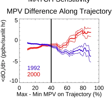
3.1. PV differences

To examine the impact of the PV difference along the back trajectories on the ozone loss rate, we bin all the data from 1992 and 2000 by the ozone loss rate and plot the mean loss rate and standard deviation for each year in Fig. 3. In the figure, data from AASE-2/EASOE appears blue while data from SOLVE/THESEO 2000 appears red.

5

The thick lines represent the mean quantities while the thin lines represent the mean plus and minus one standard deviation. The solid black line at 40% represents the filter value employed by Rex et al. (1998).

Figure 3 shows that the average loss rates are well behaved for PV differences of less than 40%. In other words, the standard deviation of the mean ozone loss rate

re-10

mains relatively constant over this domain. Beyond 50% PV differences, it is clear that neither the ozone loss rate nor the standard deviation remain constant or predictable. Therefore, the cut-off value of 40% used by Rex et al. (1998) appears to be a valid and useful parameter by which to filter out less reliable Match data.

Grooß and M ¨uller (2003) performed a sensitivity analysis of the original Match

tech-15

nique to the PV filtering criterion using the Chemical Lagrangian Model of the Strato-sphere (CLaMS). They applied a cut-off value for PV of 25% as in Rex et al. (1999) and as applied to all Match campaigns after AASE-2/EASOE in 1992. After applying the PV filter, they observe that the ozone loss rate bias that results from the original Match technique as compared to CLaMS changes from+2.40±0.07 ppbv/sunlit hour

20

to −0.41±0.08 ppbv/sunlit hour, a significant effect. We note that in their study, the Match radius is 300 km and the trajectory length is 4 days, parameters different from the original Match technique and our version of Match. Nevertheless, our results con-cur with those of Grooß and M ¨uller (2003), both indicating that the PV filter criterion is an important one for the successful application of Match. From our results a∆PV

25

cut-off of 40% may be optimal both in 1992 and in 2000, so unlike Rex et al. (2002), we do not recommend changing the cutoff to 25% for the SOLVE/THESEO 2000 study period (although to be consistent and for ease of comparison with the results of Rex et

(18)

ACPD

4, 4665–4717, 2004

Full Screen / Esc

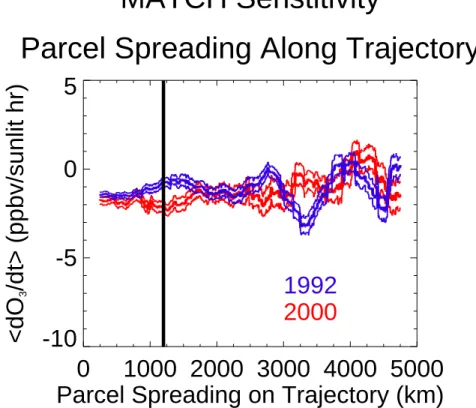
al., 1999, 2002, we do so in the studies presented below). 3.2. Cluster spreading

Next, we examine the sensitivity of the results to the spreading of the cluster of tra-jectories that was initialized for each ozonesonde observation. Rex (1993) established a criterion to filter Match data for which the trajectory of at least one member of the

5

cluster led to a separation of more than 1200 km from the central parcel at the time of the Match. Figure 4 shows the average ozone loss rate as a function of the maximum spreading of each cluster of trajectories. Again, AASE-2/EASOE is shown in blue while SOLVE/THESEO 2000 is shown in red and the thick lines represent the mean values while the thin lines represent the mean values plus and minus one standard deviation.

10

This quantity is much better behaved than the PV differences seen in Fig. 3. In fact, it is difficult to assign an appropriate distance at which a transition occurs to justify establishing a cut-off value for parcel spreading on which to filter Matches. Based on Fig. 4, it appears that the cut-off for parcel spreading need be no more restrictive than 2500 km and in fact may be entirely unnecessary. We also note that the cluster

15

spreading criterion in the original Match technique was based on parcels that started out 100 km from the central parcel, twice as far away as in our version of Match. The results of Fig. 4, therefore, should be viewed as an upper limit for the impact of this filter on the original Match technique.

Our results differ from those achieved by Grooß and M¨uller (2003). They found

20

that by applying the cluster spreading filter criterion of Rex et al. (1998), the bias in the ozone loss rate calculated in Match compared to CLaMS changes from +2.40±0.07 ppbv/sunlit hour to −0.23±0.07 ppbv/sunlit hour, another significant effect. Again, we note that the parameters used by Grooß and M ¨uller (2003) differ somewhat from those of the original Match technique and our version of Match. We also note that

25

the results of Grooß and M ¨uller (2003) are based on analysis of model data while our results are based on analysis of the actual Match data itself.

(19)

ACPD

4, 4665–4717, 2004

Full Screen / Esc

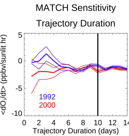
3.3. Trajectory duration

We next examine the effect of the duration of Match trajectories on the ozone loss rate calculations. Figure 5 shows the impact of including trajectories of durations of up to 14 days on the resulting ozone loss rates. As in Figs. 3 and 4, the blue lines represent AASE-2/EASOE data while the red lines represent SOLVE/THESEO 2000 data. The

5

thick lines represent the mean values while the thin lines represent the mean values plus and minus one standard deviation.

As can be seen in Fig. 5, the shortest duration trajectories show the largest variation in ozone loss rates, both in the mean and in the large uncertainties. This result is not surprising given the fact that the shortest duration trajectories will be associated

10

with the smallest exposures of the air parcels to sunlight. Since the sunlight exposure appears in the denominator of the ozone loss rate calculation, small absolute changes in these small numbers can lead to large changes in the resulting quotient.

Figure 5 indicates that no penalty is incurred with regards to the ozone loss rate cal-culations by including trajectories of durations of up to 14 days. In fact, Fig. 5 indicates

15

that the uncertainties actually decrease by including these longer duration trajecto-ries. Such a result suggests that the increased error that results from including longer, and hence more uncertain trajectories, is more than offset by the increased number of matches that result from considering more and longer trajectories. We note that al-though 14-day trajectory calculations appear at the upper end of the range of trajectory

20

durations recommended in previous trajectory studies (e.g. Morris et al., 1995, 2000) we nevertheless recommend extending trajectory calculations to 14 days for future Match analyses.

3.4. Vortex boundary

We examine the impact of the PV value at which the vortex boundary is defined.

Gra-25

dients in PV at the vortex boundary can be very strong, particularly in the Northern Hemisphere winter season. Since the precise vortex boundary is rarely clear, it is

(20)

im-ACPD

4, 4665–4717, 2004

Full Screen / Esc

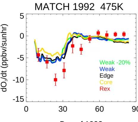
portant to examine the impact of different choices on the ozone loss rate calculations. Figure 6 shows the sensitivity of the ozone loss rate to the definition of vortex bound-ary for data from AASE-2/EASOE in 1992. In producing these loss rates, we employ only the∆PV filter. The solid colored lines represent loss rates calculated with our ver-sion of Match using four different definitions of the vortex boundary. The black curve is

5

the standard, maximum MPV gradient boundary of Nash et al. (1996) labeled “edge”. The “weak” (blue) and “core” (gold) definitions of the vortex boundary are defined by the nearest to the vortex boundary of the maximum and minimum, respectively, of the second derivative of the MPV. Finally, the “weak – 20%” is defined at the MPV value 20% less than the definition of the “weak” edge. The red squares and associated error

10

bars represent the loss rate data from Rex et al. (1998).

Figure 6 indicates that loss rates can differ by up to ∼2 ppbv/sunlit hour in January. After mid-February, loss rates seem to be consistent to within ∼1 ppbv/sunlit hour. Sys-tematic differences between the ECMWF meteorological data used by Rex et al. (1998, 2002) and the UKMO meteorological data, or differences in the precise definition of the

15

PV value at the vortex edge, therefore, could result in differences in calculated ozone loss rates.

3.5. Solar zenith angle of day/night boundary

Next, we examine the impact of the SZA definition for the day/night terminator. An examination of the sensitivity of the ozone loss rates to this quantity is relevant for more

20

reasons than the precise SZA at which the chemistry turns on and off. High sensitivity to this quantity suggests that the precise trajectory path will affect the calculated ozone loss rate. Numerous analyses of trajectory modeling have indicated that while the trajectory path computed for any individual trajectory is not reliable beyond a few days, the results from an ensemble of trajectories provides useful and reliable information for

25

much longer periods of time (e.g. Morris et al., 1995).

While a large number of trajectories is initialized in the Match technique, only a frac-tion actually are used to compute the ozone loss rates due to the numerous filters

(21)

ACPD

4, 4665–4717, 2004

Full Screen / Esc

employed by and recommended by Rex et al. (1998, 1999). According to its develop-ers, the filters of the original Match technique eliminate 30–50% of the matches (M. Rex, personal communication, 2004).

We find, however, that ≥80% of potentially matched sonde pairs and >99% of poten-tially matched sonde observations are eliminated before the ozone loss calculations. If

5

those trajectories that survive the filtering are inherently biased with regards to their po-sition relative to the local day/night terminator, a bias in the amount of solar illumination may result, biasing the calculated ozone loss rates.

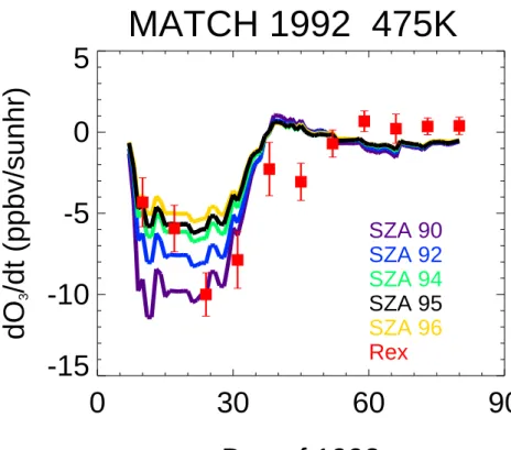
Figure 7 shows the sensitivity of the ozone loss rate to the definition of the termina-tor for data from the AASE-2/EASOE time period. In producing these loss rates, we

10

employ only the∆PV filter. The solid colored lines represent loss rates calculated with our version of Match using a range of the SZA criterion from 90◦ to 96◦. (Note that the Fig. 7 indicates little difference between the ozone loss rates computed using a 94◦ SZA criterion and 96◦ SZA criterion. Examining the difference in trajectories with SZA of 90◦ versus SZA of 94◦ lead to trajectory errors of about 4◦in latitude or 15◦ in

longi-15

tude for conditions in mid-January at 65◦N latitude. Trajectories near the vortex edge, where wind speed gradients are large, are more likely to experience such errors.) The red squares and associated error bars are again data from Rex et al. (1998). Rex et al. (1998, 2002) use a careful calculation of the exact SZA at which the sun disappears below the horizon at each air parcel altitude. In practice, that number varies very little

20

from the 95◦SZA that we employ in our version of Match. We also recall that the uncer-tainty in the trajectories themselves likely will result in larger errors than those resulting from the use of 95◦ as the SZA for the day/night terminator.

We can see in Fig. 7 that after about day 40 (9 February), the precise definition of this boundary has little impact on the calculated ozone loss rates, with variations

25

between the ozone loss rates at SZA= 90◦and that at SZA= 96◦of only ∼1 ppbv/sunlit hour. Before day 35 (4 February), however, we see large differences in the loss rate depending upon the precise SZA chosen, with the largest differences (∼6 ppbv/sunlit hour) occurring in January.

(22)

ACPD

4, 4665–4717, 2004

Full Screen / Esc

The fact that the calculated ozone loss rates show the greatest sensitivity to the SZA employed in January is not surprising. During January, the number of hours of solar illumination are quite small (and often zero) at high northern latitudes. By the middle of March, most of the same latitudes are receiving nearly 12 h of sunlight per day. As a result, the percent uncertainty in the amount of solar illumination is much greater for

5

a given trajectory in January than in March.

It is also not surprising that the largest discrepancies in the ozone loss rates calcu-lated by Rex et al. (1998, 2002) and those presented in this paper appear in January. Slight systematic differences in the trajectory calculations between the ECMWF winds used by Rex et al. (1998, 2002) and the UKMO winds used in this paper easily could

10

lead to differences in calculated ozone loss rates of 4–6 ppbv/sunlit hour in January according to Fig. 7. In fact, we see that the largest published ozone loss rate from Rex et al. (1998) for late January 1992 falls near the curve computed using a day/night terminator with a SZA of 90◦, although such a day/night terminator is unrealistic for the relevant ozone chemistry at the altitudes of our study.

15

We are led to the conclusion from Fig. 7 that the actual errors associated with the ozone loss rates calculated using Match are much larger than the statistical error bars appearing in previous publications, especially for data in January. Furthermore, the original Match technique and our version of Match include many filtering criteria, which when combined result in the selection of only a small fraction of the Match data as

20

qualifying events. Were not so many filters applied to the Match data, the likelihood of an unintentionally introduced selection bias would be substantially reduced. Figure 7 gives us cause for concern in interpreting Match results in January, particularly as related to the extremely large loss rates published by Rex et al. (1998) for AASE-2/EASOE during January 1992.

25

3.6. Sensitivity to population selection

We examine Match results after removing all the Match filters except for the Match radius and the definition of the vortex boundary using MPV. We find that the ozone

(23)

ACPD

4, 4665–4717, 2004

Full Screen / Esc

loss rates so calculated fall well within the associated uncertainties as compared to those calculated with our version of Match using all the filters combined (not shown). Furthermore, the associated error bars for the ozone loss rates are comparable if not smaller than those associated with the ozone loss rates determined in our version of Match (see discussion in Results section below).

5

Such results suggest that the five-fold increase in the number of matches which re-sults from elimination of the Match filters more than offset the added uncertainty from the inclusion of more dubious matches in the ozone loss rate calculations. Further-more, it is reassuring to include so many matches and achieve similar results. By not applying the Match filters, we can be sure that we have not accidentally thrown out

10

some good data with the bad, and we are less likely to have unintentionally biased our results. It may be reasonable to conclude that Match could be as (if not more) effective by eliminating most (if not all) of its current data filters.

In summary, our sensitivity studies indicate that the PV difference along the back trajectory appears to be a justifiable filter, and that the definitions of the vortex boundary

15

and of the SZA at the day/night terminator can have a significant impact on the ozone loss rate calculations, especially in January. (The SZA sensitivity study serves as a proxy for the sensitivity of the loss rate calculations to the precise trajectories calculated which for any individual air parcel are highly uncertain after only a few days as shown by Morris et al., 1995.) The remainder of the filters, however, do not appear to significantly

20

impact our ozone loss rate calculations.

4. Results

In this section, we present results from our version of Match (see earlier discussion for differences) and from the PV/Theta analysis. Our version of Match yields loss rates of similar magnitude to those published by Rex et al. (1998, 2002), although we are

25

unable to reproduce the largest loss rates in January 1992 on the 475 K surface without unrealistically altering the SZA for the terminator (see sensitivity study above). We also

(24)

ACPD

4, 4665–4717, 2004

Full Screen / Esc

find somewhat smaller loss rates in March 2000 on the 450 K and 500 K surfaces than those shown by Rex et al. (2002). Our loss rates do agree well with numerous other studies including model simulations, as we outline below.

4.1. Results from our version of Match

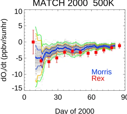
Figure 8 shows the ozone loss rate as a function of time for the SOLVE/THESEO 2000

5

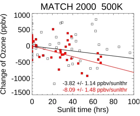
period on the 500 K potential temperature surface. Each black dot in the figure rep-resents one possible outcome for the ozone loss rate calculation (as described above and below). As an example of an ozone loss rate calculation, Fig. 9 shows the Match data from the 20-day period 12 January–1 February 2000. We randomly pick half of these matches from which to compute the line-of-best fit. The randomly selected half

10

appears as the solid red squares while the unused data are open black squares. For the red data points, we find a line-of-best-fit with a slope of −8.09±1.48 ppbv/sunlit hour. Note that this loss rate is substantially different from that calculated by using all the data of −3.82±1.14 ppbv/sunlit hour. The fact that the two slopes are ∼3 standard deviations apart suggests that such an outcome should be extremely unlikely.

Con-15

sequently, the statistical error bars probably underestimate the true uncertainty in the ozone loss rate.

Subsets of data like that shown in Fig. 9 are iteratively and randomly selected for each day (±14 days for AASE-2/EASOE or ±20 days for SOLVE/THESEO 2000). These subsets permit us to explore the range of possible ozone loss rates. Figure 9

20

represents one possible outcome. The slope computed using the data highlighted by the red squares in Fig. 9 leads to one black dot in Fig. 8. The random subsets are generated 200 times for each day. Each of the black dots in Fig. 8 therefore represents the loss rate as computed from one such subset. The mean result (the average of the black dots) is indicated by the thick blue line. The thin blue lines in Fig. 8 represent the

25

average plus and minus one standard deviation as computed using the scatter of the black dots.

(25)

ACPD

4, 4665–4717, 2004

Full Screen / Esc

minus one standard deviation as computed using the boot-strap technique (described above) to exactly one realization of the random subsets of data (e.g. the subset high-lighted in red in Fig. 9). The gold lines therefore represent a different and independent estimate of the uncertainty in the data as compared with the thin blue lines which are generated from the scatter of the ensemble of results. As expected, the uncertainty

5

from the bootstrap technique has a similar magnitude to that computed from the scat-ter of the data.

The green lines in Fig. 8 represent an estimate of the average result (thick blue line) plus and minus one standard deviation of the estimated total uncertainty. To compute the estimated total uncertainty, we add the statistical uncertainty to the uncertainty in

10

the computed loss rates generated by the uncertainty in the trajectories themselves. To estimate the uncertainty in the trajectories, we examine the impact on the ozone loss rates of changes in the SZA at which the day/night terminator is defined (see the sensitivity study above). We also add in a term to account for slightly different definitions of the vortex boundary (see the sensitivity study above). The green lines

15

are our best estimate of the total error in the loss rates as computed with our version of the Match technique.

The solid red squares in Fig. 8 represent the loss rates as calculated by Rex et al. (2002), and their associated error bars are one standard deviation from the mean as computed using standard regression error algorithms.

20

The statistical errors associated with the original Match data are similar in magnitude to the scatter in the loss rate calculations based on the subsets of data as seen in the black dots and thin blues lines of Fig. 8. However, the total uncertainty in the loss rates (green lines) is larger than that estimated by the standard regression routine (quoted with the slopes above for Fig. 9) due to the presence of other errors (see above).

Fur-25

thermore, because the regression is forced through the origin, the uncertainty estimate associated with the slope will necessarily be reduced as compared to the uncertainty in the estimate of the slope when the line-of-best fit has two free parameters (slope and intercept) as calculated with the standard routines.

(26)

ACPD

4, 4665–4717, 2004

Full Screen / Esc

For the 500 K Theta surface during SOLVE/THESEO 2000, we find reasonably good agreement between the magnitudes of the loss rates published by Rex et al. (2002) and those found in our version of Match. In late January and early February (days 15–35) and again in late February and early March (days 56–70), however, our results seem to indicate somewhat smaller loss rates than those of Rex et al. (2002).

5

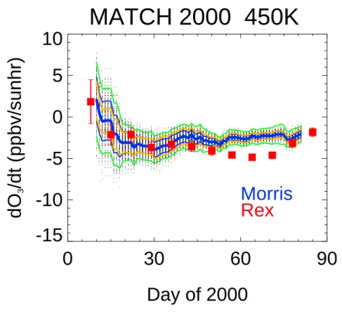
Figure 10 shows the results from our version of Match for the 450 K surface during SOLVE/THESEO 2000. While we see generally good agreement for January through mid February, we find that during days 56–84, our version of Match produces smaller ozone loss rates than those of Rex et al. (2002). Furthermore, the larger loss rates of Rex et al. (2002) in early March 2000 fall outside the statistical error bars of the Rex

10

et al. (2002) data (red) and the boot-strap (gold) and total (green) error estimates for our data. At present, we find no good explanation for the disagreement. It is possible that such differences are indicative of uncertainties inherent in the Match technique for which we have not yet accounted. As a result, we are led to the conclusion that both methods have still underestimated the actual errors of the Match technique.

15

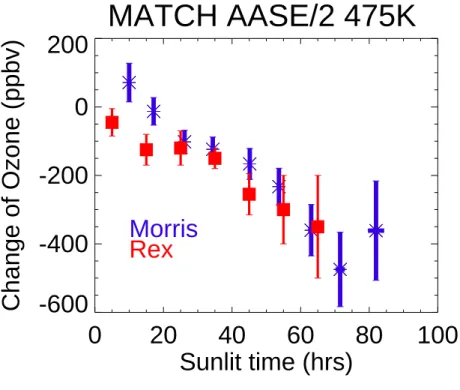
Figure 11 shows the results for the 475 K surface during the AASE-2/EASOE period of January through March 1992. We find generally good agreement throughout the period with the notable exception of days 20–35 during which Rex et al. (1998) report losses of a magnitude never before seen in the Arctic and that are difficult to repro-duce with our current understanding of stratospheric chemistry (Sander et al., 2003;

20

Solomon, 1999). Our data show large loss rates during this time period as well, but of half the magnitude. The combined uncertainty of the Rex et al. (1998) data and our boot-strap error estimates is larger than the difference in the results. However, the Rex et al. (1998) data points fall within the combined uncertainty when using our estimate of the total uncertainty (green lines), suggesting our uncertainty estimate might be quite

25

reasonable for this data. Figure 11 also shows a discrepancy for the loss rates in mid-February, again with our model showing less loss. The disagreement at this time, therefore, may be related to the differences between our vortex boundary definition and trajectories calculated using UKMO meteorological data with those of Rex et al. (1998)

(27)

ACPD

4, 4665–4717, 2004

Full Screen / Esc

calculated using ECMWF meteorological data (see the sensitivity study above). 4.2. Comparisons with other studies

Newman et al. (2002) published a summary of results for integrated ozone loss dur-ing the SOLVE/THESEO 2000 campaign on the 450 K potential temperature surface. Their Table 8 lists integrated ozone losses over the period 20 January–12 March 2000

5

from 14 different studies. Losses ranged from 0.7 ppmv (Klein et al., 2002) to 2.3 ppmv (Santee et al., 2000), with an average loss of 1.5±0.4 ppmv. Rex et al. (2002) use the original Match technique and report an integrated ozone loss of 1.7±0.2 ppmv over the same time period. Our version of Match yields an integrated ozone loss of 1.3±0.2 ppmv. (We note that the integrated loss depends upon the definition of

10

the vortex boundary.) Lait et al. (2002) use a PV/Theta approach to estimate ozone loss for SOLVE/THESEO 2000 and find an integrated ozone loss over this period of 1.7±0.3 ppmv.

No similar compilation has been published for the AASE-2/EASOE campaign for which Rex et al. (1998) and von der Gathen (1995) published their largest Arctic ozone

15

loss rates. Based on the data of Rex et al. (1998), integrated chemical ozone loss for air parcels that descended from 500 K on 1 January to 460 K on 29 February 1992 is 1.2±0.3 ppmv. For the same period, we find an integrated chemical ozone loss at 475 K of 0.8±0.2 ppmv using our version of Match. Using the PV/Theta approach, the integrated loss is 0.4±0.8 at 475 K and 0.8±0.7 at 450 K.

20

Becker et al. (1998) used a box model to calculate ozone loss rates for the win-ter/spring of 1991–1992. They found that while they are able to reproduce the Match loss rates from mid-February through March, their loss rates for the period at the end of January are significantly smaller, by more than a factor of 2, a result similar to the discrepancy we find in this study between the original Match results and the results

25

from our version of Match. The ozone loss rates of Becker et al. (1998) peak at about 4 ppbv/sunlit hour around 17 January with no indication of the large spike in loss rates found in Rex et al. (1998) for late January. The ozone loss rates of Becker et

(28)

ACPD

4, 4665–4717, 2004

Full Screen / Esc

al. (1998), however, are in quite good agreement with our results for this time period. From their Fig. 2, we see that for air parcels descending to 466 K, the ozone mixing ratio changes from about 3.85 ppmv on 1 January to 2.80 ppmv on 29 February 1992, a loss of 1.05 ppmv.

Rex et al. (2003) attempt to explain the large ozone loss rates seen in Match. They

5

use a photochemical box model run along Match trajectories. Assuming total activa-tion of chlorine, they report a maximum loss rate at 475 K in January 1992 of around 5 ppbv/sunlit hour. Such a result, while smaller by a factor of two than the reported ozone loss rates from the original Match technique, are in agreement with the maxi-mum loss rates found in our version of Match.

10

Lucic et al. (1999) use a PV/Theta approach to estimate time-integrated ozone loss at 475 K during the first 20 days of January 1992 when the vortex is well isolated (Plumb et al., 1994). They found a loss of 0.32±0.15 ppmv, which agrees with the ozone loss calculation from both the original Match approach of 0.3±0.2 ppmv and our version of Match of 0.34±0.16 ppmv. For the same period, our PV/Theta analysis indicates a loss

15

of 0.5±0.8 at 475 K.

Browell et al. (1993) report results from their differential absorption lidar (DIAL) study. They observe no polar stratospheric clouds (PSCs) within the polar vortex during the winter of 1991/1992, but do report the development of water ice (type II) PSCs just outside the vortex between Norway and Iceland on 19 January 1992. We note that

20

Rex et al. (1998) report their largest ozone loss rates five days later on 24 January 1992. The development of PSCs in this region place them upwind of a number of the European ozonesonde stations included in the Match study, perhaps impacting the results.

Using a combination of their lidar observations and a determination of the

to-25

tal amount of diabatic descent from in situ observations of trace gas species (e.g. Podolske et al., 1993), Browell et al. (1993) find a chemical ozone loss of about 23% near 460 K between January and March 1992. This percentage translates to about 0.7 ppmv of ozone, again in agreement with our integrated Match result of 0.7±0.2 for

(29)

ACPD

4, 4665–4717, 2004

Full Screen / Esc

the period 15 January–15 March 1992.

Profitt et al. (1993) use a trace gas – ozone correlation between N₂O and O₃ to deduce ozone loss in the Arctic winter vortex for 1991–1992. They report their largest ozone loss rates on 20 January 1992 of about 4.2 ppbv/sunlit hour with loss rates of 0.2–2.4 ppbv/sunlit hour throughout the rest of the winter season. These loss rates

5

agree reasonably well with the results from our version of Match, but the largest loss rate is more than a factor of two smaller than that derived from the original Match technique and published by Rex et al. (1998) and von der Gathen (1995).

Salawitch et al. (1993) use in situ observations of ClO and BrO from AASE II in conjunction with a photochemical model to determine ozone loss rates. Averaged over

10

the vortex, they find an ozone loss rate in January of 0.4% per day, notably lower than the ozone loss rates they calculate along the ER-2 flight track, which peak at 1.4% per day (about 7.5 ppbv/sunlit hour assuming 6 h of sunlight, their assumption). They report an integrated ozone loss over the entire winter at 470 K of 0.7 ppmv. Again, these calculated ozone loss calculations are consistent with our finding of 1.0±0.3 ppmv of

15

ozone loss integrated over the period from 1 January through 31 March 1992. The large difference between the vortex averaged loss rate and the peak loss rate found by Salawitch et al. (1993) suggests a possible explanation for the large ozone loss rates found in Rex et al. (1998): that localized ozone loss rates may briefly yet greatly exceed the rate characteristic of a larger geographic area.

20

Braathen et al. (1994) perform an analysis of ozonesonde data from EASOE and find an average ozone loss rate inside the polar vortex of 0.13±0.08% per day for air at 475 K during the period 9 January–12 March 1992. Rex et al. (1998) relate that the peak ozone loss rates found using the technique of Braathen et al. (1994) yield ozone loss rates of 0.8% per day in mid January, but that such rates are underestimated by

25

0.1–0.35% per day. Correcting for such an underestimate, the peak loss rates become 0.9–1.2% per day, in good agreement with the maximum rates reported using ER-2 data Salawitch et al. (1993) above.

(30)

ACPD

4, 4665–4717, 2004

Full Screen / Esc

AASE-2/EASOE mission in the winter of 1991–1992 converge on roughly the same answers: an integrated ozone loss of 0.7–1.2 ppmv between 450 K and 470 K with peak loss rates in mid-January of 4–8 ppbv/sunlit hour, with the exception of the orig-inal Match results which suggest a peak loss rate of greater than 10 ppbv/sunlit hour. Photochemical models seem to agree well with the observational data and the results

5

from our version of Match.

5. A trajectory mapping approach to Match

5.1. Methodology

We have noted that employing the various filters in our version of Match effectively eliminates ≥80% of the possible matched sonde pairs and >99% of the matched sonde

10

observations. We therefore present an alternate approach to Match that does not rely upon such filters. This approach follows from the development of trajectory mapping as employed by Morris et al. (1995, 2000), Danilin et al. (2000), and others and was first developed by Pierce et al. (1994). In this approach, all advected air parcels that arrive within the specified Match radius and within an appropriate vertical distance of

15

the new observation are considered matches with the new ozone measurement. To determine an appropriate vertical scale over which to search for matches, we calculate the autocorrelation of the noise in the ozone profile. Typically, this vertical scale is about 1 km, very similar to the 5 K vertical spacing of the Theta surfaces used in the original Match technique. In the trajectory mapping approach, however, we do

20

not compare a single observation to a single observation. Rather, we use all matches in the cylindrical volume of space around the new observation, ∼1 km in height and with a radius of 475 km (1992) or 400 km (2000) (to duplicate the Match radius criteria of Rex et al., 1998, 2002). We also permit all parcels initialized in a cluster for each ozonesonde observation to match in this approach, not just the central parcel. With the

25