HAL Id: hal-00296565
https://hal.archives-ouvertes.fr/hal-00296565
Submitted on 5 Jun 2008
HAL is a multi-disciplinary open access
archive for the deposit and dissemination of
sci-entific research documents, whether they are
pub-lished or not. The documents may come from
teaching and research institutions in France or
abroad, or from public or private research centers.
L’archive ouverte pluridisciplinaire HAL, est
destinée au dépôt et à la diffusion de documents
scientifiques de niveau recherche, publiés ou non,
émanant des établissements d’enseignement et de
recherche français ou étrangers, des laboratoires
publics ou privés.
lidar observations
K. Yumimoto, I. Uno, N. Sugimoto, A. Shimizu, Z. Liu, D. M. Winker
To cite this version:
K. Yumimoto, I. Uno, N. Sugimoto, A. Shimizu, Z. Liu, et al.. Adjoint inversion modeling of Asian
dust emission using lidar observations. Atmospheric Chemistry and Physics, European Geosciences
Union, 2008, 8 (11), pp.2869-2884. �hal-00296565�
www.atmos-chem-phys.net/8/2869/2008/ © Author(s) 2008. This work is distributed under the Creative Commons Attribution 3.0 License.
Chemistry
and Physics
Adjoint inversion modeling of Asian dust emission using lidar
observations
K. Yumimoto1, I. Uno2, N. Sugimoto3, A. Shimizu3, Z. Liu4, and D. M. Winker5
1Department of Earth System Science and Technology, Kyushu University, Fukuoka, Japan 2Research Institute for Applied Mechanics, Kyushu University, Fukuoka, Japan
3National Institute for Environmental Study, Tsukuba, Japan 4National Institute of Aerospace, Hampton, Virginia, USA 5NASA Langley Research Center, Hampton, Virginia, USA
Received: 12 October 2007 – Published in Atmos. Chem. Phys. Discuss.: 14 November 2007 Revised: 22 April 2008 – Accepted: 13 May 2008 – Published: 5 June 2008
Abstract. A four-dimensional variational (4D-Var) data
as-similation system for a regional dust model (RAMS/CFORS-4DVAR; RC4) is applied to an adjoint inversion of a heavy dust event over eastern Asia during 20 March–4 April 2007. The vertical profiles of the dust extinction coefficients de-rived from NIES Lidar network are directly assimilated, with validation using observation data. Two experiments assess impacts of observation site selection: Experiment A uses five Japanese observation sites located downwind of dust source regions; Experiment B uses these and two other sites near source regions. Assimilation improves the modeled dust ex-tinction coefficients. Experiment A and Experiment B as-similation results are mutually consistent, indicating that ob-servations of Experiment A distributed over Japan can pro-vide comprehensive information related to dust emission in-version. Time series data of dust AOT calculated using modeled and Lidar dust extinction coefficients improve the model results. At Seoul, Matsue, and Toyama, assimilation reduces the root mean square differences of dust AOT by 35–40%. However, at Beijing and Tsukuba, the RMS dif-ferences degrade because of fewer observations during the heavy dust event. Vertical profiles of the dust layer observed by CALIPSO are compared with assimilation results. The dense dust layer was trapped at potential temperatures (θ ) of 280–300 K and was higher toward the north; the model reproduces those characteristics well. Latitudinal distribu-tions of modeled dust AOT along the CALIPSO orbit paths agree well with those of CALIPSO dust AOT, OMI AI, and MODIS coarse-mode AOT, capturing the latitude at which AOTs and AI have high values. Assimilation results show
in-Correspondence to: K. Yumimoto
creased dust emissions over the Gobi Desert and Mongolia; especially for 29–30 March, emission flux is about 10 times greater. Strong dust uplift fluxes over the Gobi Desert and Mongolia cause the heavy dust event. Total optimized dust emissions are 57.9 Tg (Experiment A; 57.8% larger than be-fore assimilation) and 56.3 Tg (Experiment B; 53.4% larger).
1 Introduction
Over eastern Asia, soil dust aerosols dominate aerosol load-ing. They have important effects on the atmospheric en-vironment and climate in the springtime (e.g., Overpeck et al., 1996; Sokolik and Toon, 1996). Numerical simulations are powerful tools to elucidate dust emission, transportation, and deposition. Numerical dust models (e.g., Gong et al., 2003; Liu et al., 2003; Shao et al., 2003; Uno et al., 2004; Tanaka and Chiba, 2005) have been developed for prediction and hindcast analyses. They have provided valuable infor-mation related to characteristics of Asian dust phenomena. Nevertheless, proper estimation of dust emissions is quite difficult because of their strong dependence upon various pa-rameters (e.g., soil texture, soil wetness, land-use data, and surface wind speed). Results of the recent dust model inter-comparison project (DMIP) (Uno et al., 2006) show that sim-ulated amounts of ten-day dust emission fluxes over eastern Asia among eight dust models differed sometimes by a factor of ten. The wide scattering of dust emissions reflects differ-ences in dust emission schemes, surface boundary data, and meteorological fields within the models. Such uncertainty of estimation of dust emission fluxes strongly influences the model output.
Four-dimensional variational (4D-Var) data assimilation based on the adjoint model provides insight into various as-pects of numerical models (e.g., initial conditions, bound-ary conditions, and emissions); it has been used for meteo-rological and oceanographic modeling (e.g., Talagrand and Courtier, 1987; Benjamin et al., 2004; Awaji et al., 2003). Regarding Chemical Transport Models (CTMs), Elbern et al. (1997) and Elbern and Schmidt (1999, 2001) applied 4D-Var data assimilation to the European Air pollution Dis-persion model (EURAD), assimilating ozone observations over the European region. M¨uller and Stavrakou (2005) and Stavrakou and M¨uller (2006) presented estimates of CO and NOx emissions using the IMAGE 4D-Var system with
satellite data. Chai et al. (2006, 2007) developed a Sulfur Transport Eulerian Model (STEM) 4D-Var System and as-similated a comprehensive observation dataset during exper-iments for the International Consortium for Atmospheric Re-search on Transport and Transformation (ICARTT). Hakami et al. (2005) performed an inversion estimate of black-carbon emissions over eastern Asia using the adjoint of the STEM. Yumimoto and Uno (2006) applied 4D-Var to a regional CTM and estimated CO emissions over eastern Asia. Henze et al. (2007) developed the adjoint of GEOS-Chem and val-idated its feasibility. Dubovik et al. (2008) retrieved global aerosol sources from satellites using an adjoint of the GO-CART model. Baker et al. (2006) applied variational data assimilation for CO2. Chevallier et al. (2005) and Meirink
et al. (2006) performed inverse modeling from satellite data for CO2and methane. However, applications of 4D-Var for
CTMs remain limited.
For assimilation of dust transport, Niu et al. (2007) de-veloped a dust forecasting system using a three-dimensional variational method (3D-Var). They improved dust concen-trations with column observation data observed using the FY-2C satellite (Hu et al., 2007). However, unlike 4D-Var, 3D-Var cannot use observation data of different observation times simultaneously. Yumimoto et al. (2007) developed the 4D-Var data assimilation system of the RAMS/CFORS dust model; using NIES Lidar observations, they estimated dust emissions of a heavy dust event observed on 30 April 2005.
For the present study, we applied RAMS/CFORS-4DVAR (RC4; Yumimoto et al., 2007) to an adjoint inversion of the emission of mineral dust using NIES Lidar network observa-tion data, targeting a dense dust event observed over eastern Asia during late March and early April 2007. We conducted two experiments to evaluate effects of the selection of ob-servation sites on the assimilation results. One experiment used only observation sites located downwind of dust source regions. The other used these sites together with sites near source regions. The assimilation results were validated using various observation data. Surface PM10 concentration, the
dust extinction coefficient retrieved from Cloud-Aerosol Li-dar with Orthogonal Polarization (CALIOP) onboard Cloud-Aerosol Lidar and Infrared Pathfinder Satellite Observations (CALIPSO), MODerate resolution Imaging
Spectroradiome-ter (MODIS; aboard NASA’s TERRA and AQUA satellites), Aerosol Optical Thickness (AOT), and the Aura Ozone Mon-itoring Instrument; Aerosol Index (OMI AI) were used for validation.
This paper is structured as follows. Section 2 describes the RC4 data assimilation system. Section 3 describes the model setup and observation data used in the assimilation. Section 4 presents assimilation results and their validations. Finally, conclusions are summarized in Sect. 5.
2 Methods
The RAMS/CFORS-4DVAR (RC4; Yumimoto et al., 2007) consists of a regional dust transport model (RAMS/CFORS; Uno et al., 2003), its adjoint model, and an optimization pro-cess. In fact, RAMS/CFORS is built on a mesoscale mete-orological model, the Regional Atmospheric Modeling Sys-tem (RAMS, ver. 4.3; Pielke et al., 1992), using its optional scalar transport system and embedded dust emission, gravi-tational settling, and dry/wet deposition scheme. Thereby, all meteorological fields from RAMS are used directly for tracer advection and diffusion.
The discrete equation for the mineral dust used in RAMS/CFORS is
Q(ti+1) = M(Q(ti)) +Edt
= {I+(Madvc+Mdiff+Mreac)dt }Q(ti) +Edt, (1)
where Q is the dust concentration, M is the model opera-tor, and in which Madvc, Mdiff, and Mreacrespectively
rep-resent advection, diffusion, and reaction (including gravita-tional settling, chemical reaction and conversion, and dry/wet deposition) operators. In addition, E denotes the total dust uplift flux, t is the time, dt is the time step, and I is a unit matrix.
Strong surface winds uplift mineral aerosols into the at-mosphere. The current RC4 calculates the total dust uplift flux based on Uno et al. (2003, 2004), which uses a fourth power-law function of surface friction velocity u∗, as
Eij,k=εijCijfku3∗(u∗−u∗,t h), u > u∗,t h, (2)
where C is a dimensional constant that is a function of snow cover, soil wetness and soil texture (Uno et al., 2003); suf-fix ij denotes grid points. In addition, u∗and u∗,t h
respec-tively denote surface friction velocity and threshold friction velocity. The RC4 models 12 bin dust particles (radius 0.1– 20 µm); k denotes a bin number. Also, f signifies a fraction of each dust size bin. In this study, we introduce a scaling factor as a control vector to optimize daily dust emissions at each grid and set it equal to unity for the first guess (before assimilation).
The cost function is redefined as J (ε) = 1 2(ε − εb) TB−1(ε − ε b) + 1 2 n X i=1 (Hiε − y(ti))T R−1(Hiε − y(ti)) + γ 2 k1(ε − 1) k 2, (3)
where y denotes an observation, and H represents the for-ward model operator and the transform operator from the model space into the observation. Furthermore, B and R re-spectively denote the background error covariance and the observation error covariance. The third term is a smoothing term that is used to avoid unrealistic horizontal jumps of the control vector (Carmichael et al., 2008). γ is the strength of smoothing. The Laplacian (=∂2/∂x2+∂2/∂y2) is 1.
In fact, RC4 can include the emission scaling factor, ini-tial and boundary dust concentrations, and parameters of re-moval processes (e.g. dry deposition velocity) in a control vector. The uncertainty of numerical dust modeling includes uncertainties of emission, transport, and removal processes. At first, the uncertainty of transport depends largely on me-teorological fields. In the current version of RC4, the meteo-rological fields were provided by meso-scale model RAMS, which uses NCEP reanalysis data (already assimilated) for initial and boundary conditions, and nudging data. More-over, DMIP (Uno et al., 2006) reported that the model results correctly captured the major dust onset and cessation timing at surface observation sites; horizontal distributions of sur-face level dust concentrations appeared quite well in each model. However, the concentration levels were quite differ-ent (the difference over the Beijing region became more than 10 times greater). Secondly, Carmichael et al. (2008) esti-mated that the uncertainty of emission is 2.5 times greater than that of wet removal. On the other hand, as described in Sect. 1, the dust emission flux depends on various parame-ters; DMIP reported large variance of the emission flux for the eight numerical models. Consequently, we infer that the emission is the most uncertain, and define the emission scal-ing factor (Eq. 2) as the control vector. To reduce the uncer-tainty noise of ε, daily dust uplift fluxes are optimized.
Gradients of the cost function (Eq. 2) with respect to a set of the control vectors are necessary to minimize the function. In a 4D-Var system, the adjoint model is used to calculate them. An adjoint of Eq. (1) is derived as follows.
λ(ti) = MTλ(ti+1) +φi
=nI + (MTadvc+MTdiff+MTreac)dtoλ(ti+1) +φi (4)
Therein, λ represents adjoint variables. Furthermore, MTadvc,
MTdiff, and MTreac respectively represent adjoint operators of
Madvc, Mdiff, and Mreac. In addition, φ, which shows a
dis-crepancy between simulated and measured values (i.e. resid-ual), drives the adjoint model as a forcing term. In this study,
φ appears as φi =HTR−1(Hiε − y(ti)), (5) B Mts Ng H S Ts b) Experiment A c) Experiment B 0 150 Dust Emission (Experiment B) (ton/km ) 100 50 0 -20 100 50 Dust Emission Increments (ton/km ) Rs Sd Gn 2 2
a) Data Assimilated Dust Emission
Ty
Fig. 1. Model region and NIES Lidar observation sites. (a)
In-verted dust emission intensity from 20 March to 3 April (Exper-iment B). Circles denote NIES Lidar observation sites: Red cir-cles denote NIES Lidar observation sites used in both Experiment A and Experiment B (Tsukuba (Ts), Matsue (Mts), Nagasaki (Ng), and Hedo-Okinawa (H)). Green circles denote additional Lidar ob-servation sites of Experiment B (Seoul (S) and Beijing (B)). Blue triangles denote PM observation sites. Black circles denote WMO SYNOP observation sites. The blue box indicates a region used to produce averaged emission and wind speed (Fig. 7). (b) Dust emis-sion analysis increment of Experiment A, (c) of Experiment B.
where HT is an adjoint of H in Eq. (3). The adjoint model is integrated backward in time, and propagates the residual as adjoint variables (also called an influence function), which means that the adjoint model is also useful to perform sensi-tivity analyses (e.g. Martien et al., 2006).
In RC4, an iterative optimization routine, which applies Quasi-Newton L-BFGS (Liu and Nocedal, 1989), is used to minimize the cost function. That optimization routine re-quires several integrations of both forward and adjoint mod-els before a convergence criterion is satisfied. Meteorologi-cal fields are generated in advance by RAMS. Pre-Meteorologi-calculated RAMS meteorological fields drive the forward and backward models in an off-line manner to reduce computational loads. Consequently, in the current version of RC4, the meteorolog-ical fields (e.g., temperature and humidity) have no feedback of the tracer field and were not assimilated. The convergence criterion is that the norm of the gradient of the cost func-tion is reduced by a factor of 1000 with respect to the initial one, meaning that another iteration would produce little dif-ference. In this study, we had around eight iterations.
3 Experiment setup and observations
Based on dust extinction coefficients measured by the NIES Lidar observation network, RC4 is applied for assimilation
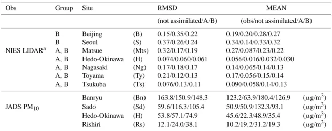
Table 1. Observation sites of NIES Lidar and JADS PM measurements: RMS differences between observed and modeled values, with mean
values at each site (29 March–4 April).
Obs Group Site RMSD MEAN
(not assimilated/A/B) (obs/not assimilated/A/B)
B Beijing (B) 0.15/0.35/0.22 0.19/0.20/0.28/0.27
B Seoul (S) 0.37/0.26/0.24 0.34/0.14/0.33/0.32
NIES LIDARa A, B Matsue (Mts) 0.32/0.17/0.19 0.27/0.087/0.23/0.22
A, B Hedo-Okinawa (H) 0.074/0.060/0.061 0.056/0.016/0.032/0.030 A, B Nagasaki (Ng) 0.17/0.18/0.17 0.14/0.065/0.14/0.13 A, B Toyama (Ty) 0.21/0.12/0.13 0.17/0.056/0.15/0.14 A, B Tsukuba (Ts) 0.076/0.13/0.11 0.090/0.058/0.14/0.13 Banryu (Bn) 163.8/150.9/148.3 123.2/63.9/180.4/126.9 (µg/m3) JADS PM10 Sado (Sd) 59.6/116.3/105.4 50.9/50.9/132.3/93.1 (µg/m3) Hedo-Okinawa (H) 53.8/57.1/74.9 45.6/22.3/48.9/35.4 (µg/m3) Rishiri (Rs) 12.1/24.0/38.1 10.2/19.2/31.2/19.3 (µg/m3)
aRMS differences (RMSD) and mean values are computed based on the dust AOT calculated by integration of the dust ext. coefficients.
of dust observations and inversion of dust emissions over eastern Asia. Figure 1a shows the simulation area, which is centered at 37.5◦N, 115◦E on a rotated polar stereo-graphic system. The horizontal grid comprises 180×100 grids with 40 km resolution. The vertical grid comprises 40 grid points extending from the surface to 23 km with 40 stretching grid layers (140 m at the surface to 650 m at the top) in terrain-following coordinates. Meteorological bound-ary conditions to RAMS meteorological integration are taken from NCEP/NCAR reanalysis data with 2.5◦×2.5◦ resolu-tion and a 6 h interval. For this study, the simularesolu-tion is per-formed during 20 March–4 April 2007 with zero initial dust concentration.
At 14 locations, NIES Lidars (Sugimoto et al., 2006; http://www-lidar.nies.go.jp/) are operating continuously (see Fig. 1a), measuring vertical profiles of dust outflows over eastern Asia with high spatial and temporal resolution. Their vertical and temporal resolutions are, respectively, 30 m and 15 min. The extinction coefficient is derived based on the backward Fernalds method (Fernald, 1984) by setting a boundary condition at 6 km. We used a non-zero bound-ary value when the retrieved aerosol profile was negative (Shimizu et al., 2004) setting the Lidar ratio S1=50 sr (Liu et al., 2002). Then the dust extinction coefficient is derived from the extinction coefficient using the contribution of min-eral dust, which is estimated using the particle depolarization ratio (Shimizu et al., 2004).
In this study, the vertical profiles of the dust extinction co-efficients are assimilated directly. They are used to evalu-ate the cost function (Eq. 3). Modeled dust extinction co-efficients are calculated based on Takemura et al. (2000) at every model time step. We performed two assimilation ex-periments to evaluate impacts on the assimilation results of the choice of observation sites. Experiment A assimilates
five Lidar sites over Japan that are located downstream of the dust source regions. Experiment B assimilates those five sites and another two sites, including sites downstream from and proximate to the dust source region. Consequently, Experi-ment A includes data of Hedo-Okinawa, Nagasaki, Matsue, Toyama, and Tsukuba. Experiment B uses data of the five sites of Experiment A, with additional data from Beijing and Seoul (Table 1). Observation sites of each set are shown as bold circles in Fig. 1a (red circles represent observation sites used in both Experiment A and Experiment B; green circles represent sites added to Experiment B). The Lidar data are interpolated vertically to the RC4 vertical resolution. Then 1-h averaged Lidar dust extinction coefficients are used for data assimilation with a 3-h interval. For both observation groups, the dust extinction coefficients measured from 29 March to 4 April 2007 from the surface to 4000 m altitude were assimilated. For this study, surface observations (e.g. PM10 observations) and satellite data (OMI AI, CALIPSO
Lidar data, and MODIS aerosol optical thickness) were used only for validation: those data were not applied to data as-similation. The current RC4 can assimilate these observation results. Introduction of these data will be the next step of our application in future studies.
Accurate estimation of the background error (B) of the dust emission flux is important for adequate data assimila-tion. The dust uplift flux depends on numerous parameters (e.g., soil texture, soil wetness, land-use data, and surface wind speed). In addition, dust emissions over the inland desert region have been measured sparsely. These facts ren-der the estimation of the background error (B) of dust emis-sion extremely difficult. Uno et al. (2006) suggest that dust emission fluxes over eastern Asia differ immensely among the DMIP 8 models. The dust emission fluxes over east-ern Asia (including the Gobi desert, Inner Mongolia, and the
Fig. 2. Comparison of horizontal distributions of modeled AOT and OMI AI: the left column shows modeled dust AOT from assimilation
Experiment B (color) and OMI AI (pink lines; interval = 1, 3, 5); the right column shows model dust AOT without assimilation (color) and SYNOP dust report (pink $ symbols).
Taklimakan Desert) were 27–336 Tg with a mean of 120 Tg for period A (15–25 March 2002), and 18–103 Tg with a mean of 36.3 Tg for period B (4–14 April 2002), reflect-ing various differences among the models (e.g., dust emis-sion scheme, surface boundary data (e.g., soil texture, soil moisture, and snow cover data), and meteorological fields). The maximum of the dust emission flux of DMIP is some-times about 600–1200% of the minimum. In the develop-ment stage of our system, we performed several sensitivity experiments changing the uncertainty of the dust flux from 1000% to 50%. Uncertainty of 500% engendered reasonable and realistic results that were appropriate for the variations of dust fluxes of DMIP models. In this study, the background error covariance (B) for the dust emission is assumed as diag-onal, with assigned uncertainty of 500% to the dust emission
flux as the background error. Measurements near the source region and a detailed evaluation of the background error will help to improve the model prediction and its assimilation.
The observation error covariance (R) is assumed to be di-agonal. Sugimoto et al. (2002) estimated the error introduced by the assumption of the Lidar ratio (S1). The extinction co-efficient using S1=50 sr was increased by 16% compared to that using S1=40 sr, and decreased by 11% compared to that using S1=60 sr at 1 km altitude. Using the relative error alone engenders extremely small observation error and prevents the assimilation procedure from converging on the optimized so-lution. In this study, we introduced a minimal absolute error and defined the observation errors as
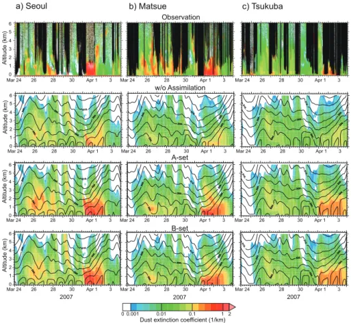
a) Seoul b) Matsue c) Tsukuba Observation Observation w/o Assimilation A-set B-set 0.001 0.01 0.1 1 2 Dust extinction coefficient (1/km)
Observation 2007 2007 2007 5 6 4 3 2 1 0 Altitude (km) 5 6 4 3 2 1 0 Altitude (km) 5 6 4 3 2 1 0 Altitude (km) 5 6 4 3 2 1 0 Altitude (km) 28 30 Apr 1 3 26
Mar 24 Mar 24 26 28 30 Apr 1 3 Mar 24 26 28 30 Apr 1 3
28 30 Apr 1 3 26
Mar 24 Mar 24 26 28 30 Apr 1 3 Mar 24 26 28 30 Apr 1 3
28 30 Apr 1 3 26
Mar 24 Mar 24 26 28 30 Apr 1 3 Mar 24 26 28 30 Apr 1 3
28 30 Apr 1 3 26
Mar 24 Mar 24 26 28 30 Apr 1 3 Mar 24 26 28 30 Apr 1 3
0
Fig. 3. Time-Height plots of dust extinction coefficients (log-scaled) at Seoul, Matsue, and Tsukuba. The first row shows NIES Lidar
observations. Blacked-out areas represent missing data attributable to the presence of clouds, rain, or heavy dense dust layers which the Lidar signal cannot penetrate. Second, third, and fourth rows respectively show modeled dust extinction data without assimilation, assimilated (Experiment A), and assimilated (Experiment B).
where Rabs represents a minimal absolute error set as
0.05 km−1; R
relrepresents the relative error rate, which was
assigned as 10%.
To avoid the unrealistic jumps, using correlation elements of the background error might be useful and physically more meaningful. However, an application of the correlation of the background error matrix will require more sensitivity studies. So we want to keep this sensitivity analysis as a next step of our study. The strength of smoothing γ (=10 000 (m4)) is decided through sensitivity analyses with another dust event during the develop stage of the system. In this study, final fractions of the background error and the smoothing terms converged on 10% and 0.5% of the final value of the cost function (after the convergence), respectively.
In the dust event targeted by this study, the forward dust model (without the assimilation) generally underestimates the dust concentrations (see Figs. 3 and 4), and slightly nega-tive values occurred through the both adjoint inversions. We assumed that the negatives are negligible; they were replaced with zero emissions.
4 Results and discussion
4.1 Assimilation results
Figure 2 portrays horizontal distributions of modeled AOT and the OMI AI. In the left column, colored and pink con-tours respectively denote assimilated AOT and OMI AI. In the right column, color represents model dust AOT with-out assimilation. The symbol $ shows the dust report from the WMO SYNOP surface weather. Figure 1 shows all SYNOP stations throughout eastern Asia. In fact, OMI AI is also sensitive to non-dust aerosols; high AI levels observed over southern Asia are attributed to aerosols originating from biomass burning (e.g. black carbon). For 1 April, OMI AI data are not available.
A low-pressure area in northeast Mongolia on 30 March created strong surface winds that bore high-density dust aloft over an extended desert region including north-central China and Mongolia. The dust was subsequently transported to the east with the low-pressure system and its accompanying cold front. It reached northeast China on 31 March, extending from the East China Sea to the Sea of Japan on 1 April. It
covered the islands of Japan on 2 April. The modeled AOT coincides well with OMI AI and SYNOP dust reports. Gen-erally, the modeled AOT is increased by assimilation. The assimilation results reproduce dense dust loadings centered near 105◦E and 40◦N on 30 March and covering Japan on 1 April, which was not reproducible using the simple CFORS model.
Figure 3 shows comparisons of observed and modeled dust extinction coefficients at Seoul, Matsue, and Tsukuba. The first and second rows respectively show observations and model results without assimilation. Blacked-out areas in ob-servations show missing obob-servations. Contour lines repre-sent the potential temperature by RAMS. A heavy dust event occurred from 31 March to 1 April at Seoul (dust extinction coefficients were greater than 2 km−1), and from 1 April to 2 April at Matsue and Tsukuba. Figure 2 shows that dense dust loading occurred; the dust was trapped by the low-pressure system and its accompanying cold front, which approached Mongolia and north-central China on 30 March 2007, then continued eastward. The dust events observed at each Lidar site are presumed to have detected dust transported by this low-pressure system and its associated cold front. Other ob-servation sites throughout Japan detected a similarly dense dust layer, which arrived between 1 and 2 April with a dense dust extinction coefficient level (>1 km−1). Model results without assimilation represent the onset and overall behav-ior of the dust layer, but the dust extinction coefficients are underpredicted considerably during the heavy dust event.
The lower two rows in Fig. 3 show assimilation results. The third row shows the results of Experiment A; the fourth row shows results of Experiment B. The assimilation results compensate model dust extinction coefficients considerably and bring modeled concentrations closer to observed ones. At the Tsukuba observation site, two dust peaks observed on 1 and 2 April are reproduced and emphasized by the assim-ilation. The structures and onset timings of the dust layers are not modified dramatically. The forward model itself pre-cisely represents dust emission timings and source regions. Consequently, the assimilation need not adjust those consid-erably, but it improves the emission intensity.
At Seoul (Fig. 3a), dense dust layers were observed on 31 March and 1 April. The Lidar was not able to measure dust at altitudes greater than 2000 m at Seoul between 31 March and early 1 April because the signal was not able to penetrate the very dense dust below that altitude. This fact indicates that dust loading observed at 2000–3500 m height on 1 April is continuous (not separated) with the dense dust layer on 31 March. The model reproduces the dust layers, including dense dust in upper layers between 2000–3500 m on 1 April. At the Matsue observation site (Fig. 3b), the model cap-tures the dense dust loading that occurred between 31 March and 2 April; considerable improvements of the model dust extinction coefficients are apparent during the dense dust loading through assimilation. However, the assimilation re-sults were incapable of reproducing an elevated dust layer
on later 30 March at 3000–4000 m altitude (a similar dust layer is observed at Nagasaki; not shown). The HYSPLIT trajectory model (Draxler and Hess, 1998; http://www.arl. noaa.gov/ready/hysplit4.html) suggests that the air masses corresponding to the dust layers originated above the Tak-limakan Desert region (not shown). That region, located in western China, is surrounded by high mountains: the Tian Shan Mountains, Pamir Plateau, Tibetan Plateau, and Kun-lun Mountains. Because of its complicated and sharp terrain, it is difficult to reproduce detailed meteorological fields (es-pecially, wind speed and direction, and the boundary layer height; Uno et al., 2005). The resolution of the current RC4 (40 km) might not be sufficient to reproduce the dust emis-sion and uplifting of the dust particles resulting from the to-pography conditions (i.e., surface winds, updraft along the sharp terrain, and convection). The difficulty of meteoro-logical simulation prevented assimilation from modifying the dust emission over this region because the adjoint model can-not propagate the required dust emission information (i.e. the residual) to the control vector ǫ in Eq. (2) backward in time. Improvement of RAMS horizontal resolution might improve the assimilation performance.
Little difference is apparent between results of Experi-ment A and ExperiExperi-ment B. The Seoul observation site data are not used in Experiment A. Nevertheless, the Experi-ment A assimilation results improve the model dust extinc-tion coefficient considerably; dramatic improvement is not obtained from Experiment B. Observation sites in Experi-ment A are distributed widely over Japan along the meridian, which is perpendicular to the main dust outflow direction. This fact indicates that the observation data of Experiment A captured the dust event characteristics extensively and ade-quately, and increased the assimilation performance. The ex-istence of only slight differences between results of Experi-ment A and ExperiExperi-ment B also indicate that the assimilated emission by Experiment A is consistent with Lidar-observed results at Seoul and Beijing. The assimilated emissions are discussed in Sect. 4.4. Results of Experiment B are presented as our “assimilation results” in the following sections.
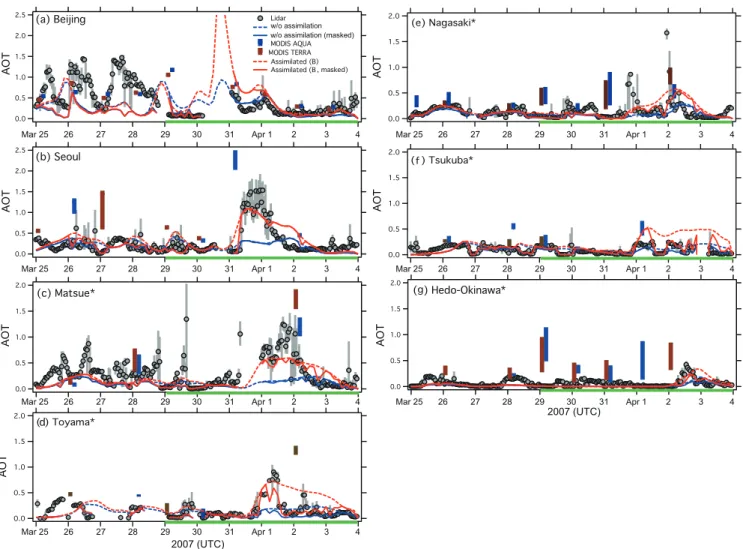
Figure 4 shows time series data of dust aerosol optical thickness (AOT) at Lidar observation sites. The dust AOT is calculated through vertical integration of the dust extinc-tion coefficient from the surface to 6000-m altitude. The total and coarse mode AOTs derived from the aerosol opti-cal depth and the aerosol optiopti-cal depth ratio provided by the Level-3 MODIS Atmosphere Daily Global Product (Remer et al., 2005) are also shown. It is noteworthy that the MODIS coarse mode AOT is also sensitive to non-dust aerosols (e.g. sea salt).
On 31 March, a dense dust loading was observed at Seoul. This dust loading is presumed to have reached the Beijing site on 30 March. However, weather conditions obscured the observation data. Over the Japanese islands, the dust layer was first observed at Matsue and Toyama on 31 March, then detected at Nagasaki and Tsukuba on 1 April; it finally
Fig. 4. Time series of Lidar and modeled, MODIS AOT at NIES Lidar sites. Circles denote the 1-h-average of dust AOT calculated using
Lidar observations. Gray bars denote ranges between minimum and maximum of Lidar dust AOT. Red lines show assimilated dust AOTs; blue lines are those without assimilation. Dashed lines denote modeled AOTs by the full integral from the surface to 6 km height. Solid lines denote modeled dust AOTs calculated by the partial integrals, which is only taken over the height range in which Lidar observations are presented. Blue and orange box bars denote ranges between total AOT (box top) and coarse mode AOT (box bottom), as measured by MODIS. Observation data measured during 29 March–4 April are assimilated (shown as green horizontal lines).
reached Hedo-Okinawa on 2 April. The MODIS observa-tions also measured heavy dust loading at each observation site. The model well reproduced those onsets of dust loading. The assimilation results improve the modeled dust AOT and agree quite well with Lidar dust AOT. Time variations between Lidar AOT and MODIS AOT show good agreement; the assimilation results also capture these variations well. The assimilated dust AOT is increased by 2–2.5 times com-pared to that before the assimilation during the dust event, which hit Beijing on 30 March, Seoul between 31 March and 1 April, and Japanese sites on 12 April.
At the Beijing observation site, because of cloudy and rainy conditions that persisted from 29 March to early 31 March, the Lidar measured few vertical profiles of the dense dust layer. Between 25 March and 28 March, the simulated dust AOT remained underestimated compared to the Lidar
dust AOT. These high Lidar dust AOT levels might reflect local dust storms and local air pollution, which were unable to reach Seoul and Japanese sites. Assimilations including observation data measured during that period might improve such differences. On 31 March, the Nagasaki and Matsue Lidars detected dense dust that the model was unable to re-produce. As described previously, these elevated dust layers might have originated from the Taklimakan Desert region.
Table 1 presents the root mean square (RMS) of differ-ences between the observed and modeled AOT from 29 March to 4 April, as well as the mean AOT values. Data assimilation improved the RMS differences and the biases between observed and modeled mean values. At Seoul, Toyama, and Matsue, the RMS differences are reduced by 29–47% in Experiment A and 35–40% in Experiment B. Experiment A shows significant improvement of the RMS
differences and the mean value of Seoul. At Beijing, Tsukuba, and Nagasaki, the mean AOT values are brought much closer to observed ones. However, the RMS differ-ences are not improved in spite of the assimilation. At Bei-jing, the relative lack of data available during the heavy dust event might engender that result. At Nagasaki, dust loading from the Taklimakan Desert observed on 31 March might re-sult in the smaller improvement of the RMS difference. At the Tsukuba site, the observation data of the heavy dust event are fewer than those at other observation sites because of high clouds and rain (see Fig. 2c), which might explain the degra-dation of the RMS difference.
4.2 Surface measurements
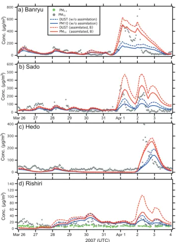
Validation of the assimilation results by observations that were not used for the assimilation is crucially important. Fig-ure 5 shows comparisons of time series of surface PM10 at
Rishiri, Banryu, Sado, and Hedo-Okinawa (shown as blue triangles in Fig. 1a). Hourly PM10 and PM2.5 (at Rishiri
only) observations were provided by the Japan Acid Deposi-tion Survey (JADS) of Japans Ministry of the Environment. Dashed lines denote total dust concentrations; solid lines denote dust PM10 concentrations calculated from the eight
smaller bins, with 0.13, 0.21, 0.33, 0.52, 0.82, 1.27, 2.01, and 3.19 µm effective radii, respectively.
The heavy dust layer was measured on 31 March at Ban-ryu and Sado; it then reached Hedo-Okinawa and Rishiri. At Rishiri, the peak concentration of the dust layer is much less (ca. 40 µg/m3) than at the other sites (ca. 300–800 µg/m3) because the dust layer is elevated toward the north, as de-scribed in the following Sect. 4.4. Two peaks of concentra-tions are visible at Banryu and Sado, which are also observed at the Tsukuba Lidar site (see Fig. 3c). The model reproduces these peaks.
Considerable improvements are apparent in PM10 peak
concentrations despite the assimilation using only Lidar ob-servations. The modeled peak concentrations are doubled or tripled by the assimilation, and show good agreement with observations. At Hedo-Okinawa, the assimilation results in-duce the onset time of model PM10peak to come 3 h earlier
and occur closer to the observed onset time. In contrast, the assimilated PM10slightly overestimates the observed one at
Rishiri. In this study, Experiment A and Experiment B did not include a Lidar observation site located in the north re-gion, that at Sapporo (Fig. 1). Because of rain and clouds, the Sapporo Lidar obtained little observation data during the dust event. Further improvements, especially over the north region, can be expected if such measurements are used for assimilation.
Table 1 also shows the RMS differences and mean values of PM10 concentrations. At Banryu, the assimilations
im-prove the RMS difference and bring the modeled mean con-centration closer to the observed one. However, at the other station, the RMS differences are degraded. In Fig. 5, the
Fig. 5. Comparison of modeled (without assimilation and
assimi-lated) and observed surface PM10concentrations at Rishiri, Banryu,
Sado, and Hedo-Okinawa. Circles show hourly PM10 and PM2.5
(at Rishiri only) observations. Dashed lines denote modeled dust concentrations; solid lines show modeled dust PM10concentrations
calculated with eight smaller bins.
observations show a very rapid decrease of PM10
concentra-tions at offsets of the dust event. Although the peak PM10
concentrations are improved, the assimilations also engender overestimation of the concentrations after the peak. Degrad-ing of the RMS differences caused by this overestimation after the peak overcomes improvement of RMS differences through better agreement of the peak PM10, resulting in the
total degradation of the RMS differences. The model resolu-tion might be insufficient to reproduce the observed sharp peaks. Because of the smaller emission amount, Experi-ment B yields better RMS differences than those achieved through Experiment A (Sect. 4.4).
4.3 Space-based lidar
A space-based backscatter lidar, CALIOP, was launched on-board CALIPSO on 28 April 2006 (Winker et al., 2007). As an active instrument in space, CALIOP is currently provid-ing continuous global measurements of aerosol and cloud
vertical distributions. The CALIOP data products are there-fore an ideal data source for validating the vertical structure of the assimilated dust event. In this section, we compare the assimilation results to the CALIOP products to evaluate our assimilation system.
In fact, CALIOP provides profiles of the total attenuated backscatter coefficient at 532 nm and 1064 nm, in addition to the depolarization ratio at 532 nm in the Level 1B data products at horizontal resolution of 333 m. Both vertical and horizontal resolutions vary for different altitude ranges be-cause of the onboard averaging to reduce the data volume to be downlinked. The CALIOP Level 2 data processing finds features (cloud, aerosol, surface, etc.) in a lidar profile and classifies the features. Currently released in the Level 2 layer products are the layer-averaged attenuated optical prop-erties along with cloud-aerosol discrimination (CAD) results. The CAD score is computed based on the cloud and aerosol probability density functions (PDFs) and is used as an in-dicator for discrimination between clouds and aerosols for the CALIOP layer (Liu et al., 2004). It ranges between
−100 and 100: positive values denote clouds, whereas neg-ative values denote aerosols. The absolute value of the CAD score signifies a confidence level for the classification. De-tailed descriptions can be found on the CALIPSO web page (http://www-calipso.larc.nasa.gov/) and references therein.
The extinction retrieval is not released in the current Level 2 data products. Therefore, we retrieved dust extinction co-efficients from the CALIOP LEVEL 1B data using the same method as that used for NIES Lidar described earlier. The forward inversion is started from 14 km height down to the ground surface with S1=30 sr. For this study, the dust extinc-tion coefficients derived from the CALIOP measurements are averaged to the horizontal resolution of Level 2 (5 km).
Figure 6 shows CALIPSO observations and model results. Each CALIPSO path overpasses near the center of the dense dust layer with a low-pressure area; its cold front is as shown in the first row of Fig. 6. The dense dust layer emitted from north-central China and the Mongolia region moved east-ward and reached the Sea of Japan on 1 April. On paths A, B, and C, the model results (second row of Fig. 6) show that the dust layer is elevated to the north along the isen-tropic surface of θ =290–300 K as it travels eastward. In ad-dition, CALIPSO (third row of Fig. 6) captures that elevated dust layer and agrees well with the model results. On path D (Fig. 6d), CALIPSO observed the dust layer over the Yellow Sea; the model also captured the dust layer.
The CAD scores (fourth row of Fig. 6) characterize the CALIOP layers with high dust extinction coefficients as vague (near-zero values). For dense dust layers, because of their high backscatter coefficient and color ratio (simi-lar to those for optically thin clouds), they generally fall in the overlap/vague region of the aerosol and cloud PDFs; the magnitude of CAD scores for this type of aerosol is gener-ally near zero, as demonstrated by the dust layers (greenish in the CAD scores) between 38◦N–46◦N on path A, 34◦N–
42◦N on path B, and 38◦N–43◦N on path C in the fourth
row of Fig. 6. In this case, misclassifications can occur. Liu et al. (2004) suggested that misclassification can also hap-pen when the aerosol layer is contaminated by embedded or vertically adjacent clouds. In Fig. 2 and the first row of Fig. 6, we show that the dust plume occurred following the passage of the low-pressure area and its accompanying cold front; CALIOP observed the area adjacent to them on path B (Fig. 6b), and close behind them on path A (Fig. 6a) and path C (Fig. 6c). Heavy dust loading (AOT>2) occurs adja-cent to the cold front and co-exists with the ice-cloud, which complicates the dust classification. The cloud and aerosol discrimination results currently released in the Level 2 layer products are beta version: they are early release products for users to gain familiarity with data formats and parameters. This data product must be validated. The CAD algorithm is being refined for future data releases.
The fifth row in Fig. 6 presents a comparison of the mod-eled dust AOT, CALIPSO dust AOT, OMI AI, and MODIS coarse mode AOT interpolated along each orbit path. The modeled and CALIPSO dust AOT are calculated through ver-tical integration of the dust extinction coefficient from the surface to 14 km. The modeled and MODIS AOTs corre-spond to the left axis, CALIPSO AOT correcorre-sponds to the right inside axis, and OMI AI corresponds to the right axis. On 1 April, OMI AI was unavailable. Satellite observa-tions are available once daily: MODIS TERRA overpasses at 10:30 LT (about 02:00 UTC over eastern Asia), MODIS AQUA crosses at 13:30 LT (about 05:00 UTC over eastern Asia), and OMI overpasses at 13:45 LT (about 05:00 UTC over eastern Asia).
In general, the modeled and observed AOT show good agreement, capturing the latitude at which AOTs and AI have high values. Both MODIS TERRA and AQUA coarse mode AOT, and modeled dust AOT are quantitatively con-sistent. Some dips are apparent in the observations. For example, in path A, two peaks that are not found in model results are produced by a dip around 40◦N in CALIPSO dust AOT and OMI AI. This dip is caused by a cloud at 10 km height (see fourth row). Similar observation dips are visible around 39◦N and 44◦N–48◦N on path B, and around 40◦N and 43◦N on path C. On paths B and D (Fig. 6b and d), which cross over the Yellow Sea and near industrial regions of east China, satellite observations measure high AOT and AI (e.g., MODIS and OMI observations around lower lati-tudes on path B, MODIS TERRA observations on path D). These high values might be partly affected by pollution from the industrial region of east China.
Compared to modeled and MODIS coarse mode AOT, CALIPSO dust AOT is lower. Particularly on paths A, B, and C, the upper dense dust layers (AOT>2) hampered penetra-tions of CALIPSO Lidar signals to the lower layers, thereby engendering underestimation of CALIPSO dust AOT. Fur-thermore, the assigned S1 value (S1=30 for this study) might partly affect the underestimation.
Fig. 6. Comparison of modeled and CALIPSO dust extinction coefficients. The first row shows CALIPSO observation paths and modeled
dust AOT (Experiment B) and surface winds. L shows the low-pressure area; red broken lines represent the cold front. The second row shows modeled dust extinction coefficients (color) and potential temperature (white line) along the CALIPSO observation path. The third row shows the CALIPSO dust extinction coefficient (color); broken lines show the modeled dust extinction coefficient (0.5, 1.0, 1.5, 2 km−1). The fourth row shows the CAD score. The fifth row shows the modeled dust AOT (left axis), CALIPSO dust AOT (right inside axis), MODIS coarse AOT (left axis), and OMI AI (right axis) along the CALIPSO path.
4.4 Dust emission
Figure 1 shows assimilated dust emission intensities from 20 March to 3 April. Figure 1b and c respectively depicts in-crements obtained using results of assimilation for Experi-ment A and ExperiExperi-ment B. Both results increase dust emis-sions over the Gobi Desert and Mongolia; especially around the border between China and Mongolia. Despite the close similarity of distributions of increments of dust emission fluxes obtained by Experiment A and Experiment B, some differences exist. These differences might reflect more de-tailed data related to dust storms observed at Beijing and Seoul, which were not observed over Japan (e.g. a dust storm observed at Beijing on 3 April (see Fig. 4a)). Meanwhile, the close similarity of flux distributions indicates that the as-similation results of Experiment A are consistent with obser-vations made at Beijing and Seoul. Moreover, an assimila-tion using Experiment A observaassimila-tions can obtain appropri-ate assimilation results for severe dust storms. As described earlier, the NIES Lidar observation network, which is dis-tributed widely over Japan, enables Experiment A to capture the overall behavior of the dust event. Additionally, obser-vations near the dust storm regions (e.g., Beijing, Seoul, and other new Lidar sites) can include more detailed dust storms in assimilations, and might become crucial for real-time fore-casting using a 4D-Var assimilation system.
Figure 7 shows the daily variation of dust fluxes as well as the averaged wind speed, u∗and u∗,t h, in the dust source
region (see Fig. 1a). Between 29 and 30 March, the assim-ilation increases the dust flux considerably. On 29 and 30 March, the model simulated high wind speeds and u∗. A
strong wind blew over Mongolia and north-central China to the northwest; it lifted up enormous amounts of dust parti-cles into the atmosphere. On those days, the assimilation increases dust emission flux by 2–3 times, indicating that the heavy dust storm results from this strong surface wind over those regions on 29 and 30 March. We obtained the total opti-mized dust emissions of 57.9 Tg (Experiment A, 58% larger than without the assimilation) and 56.3 Tg (Experiment B, 53% larger than without the assimilation) during the assimi-lation window.
Most grid cells in which dust fluxes are increased consid-erably by the assimilation are designated as having a loamy sand soil texture (not shown). In the current RC4, the ini-tial dust-size distribution of the dust uplift flux is the same in all dust-emission regions. The assimilation results might reflect this poor information about the dust-size distribution. As a future task, optimization of the dust-size distribution at each model grid cell might be necessary. However, few ob-servations provide dust size distributions. Expansion of such observations is both important and necessary.
Fig. 7. Daily dust emission flux and regional averaged modeled
wind field at lowest model grids and u∗, and u∗,t hthroughout the region depicted in Fig. 1a.
5 Concluding remarks
Adjoint inverse modeling using the regional dust model was applied to the dust event that occurred over eastern Asia be-tween 20 March and 4 April 2007. The vertical profile of the dust extinction coefficients derived from Lidar observations was assimilated directly. We performed two assimilation ex-periments to evaluate the impact of observation site selec-tions on assimilation results: Experiment A used five obser-vation sites distributed throughout Japan (downstream of the dust source region); Experiment B used those five observa-tion sites and two other sites nearer the dust source region (Beijing and Seoul). The assimilation results were validated using various observation data: MODIS coarse mode AOT, CALIPSO dust extinction coefficient, OMI AI, the WMO SYNOP weather report, and surface PM10 concentrations.
Results can be summarized as follows:
1. Dense dust loading originated from a desert region that extended over north-central China and Mongolia. On 30 March, that region was swept by a low pressure system and its accompanying cold front. The resultant dust, borne aloft, reached the East China Sea and the Sea of Japan on 1 April; it covered the Japanese islands on 2 April. The modeled AOT coincides well with data of these dust onsets and aerosol distributions measured by OMI AI. The assimilation increases the modeled AOT
and reproduces the dense dust loading, which was not captured before the assimilation.
2. The modeled dust extinction coefficients are improved considerably and come to explain Lidar dust extinction coefficients after assimilation. The assimilation results of Experiment A are consistent with those of ment B. This fact indicates that observations of Experi-ment A can capture the dust layer comprehensively. 3. Time series of dust AOT by the model can capture both
Lidar and MODIS coarse mode AOT variations well. Assimilation results increase modeled dust AOT and improve peak dust AOT levels markedly. At Seoul, Toyama, and Matsue, the RMS differences of dust AOT are reduced by 35–40%. However, at Beijing and Tsukuba, the RMS differences degrade because of fewer observations during the heavy dust event. Exper-iment A also showed improved RMS differences and mean AOT values at Seoul (not included in Experi-ment A).
4. Surface PM10 concentrations from the Japan Acid
De-position Survey (JADS) are used for independent vali-dation of the assimilation results. The model can gen-erally capture variations of observations and reproduce unique characteristics of two peak PM10concentrations
measured at Banryu and Sado. The assimilation results double or triple the modeled peak concentrations dur-ing the heavy dust event and show good agreement with observations. At Banryu, the RMS difference between modeled and observed PM10 is improved. However,
at Sado, the RMS differences are degraded, indicating that the model resolution was insufficient to reproduce observed sharp peaks, especially at the end of the dust event.
5. The assimilation results are compared with dust ex-tinction coefficients retrieved by CALIPSO (a satellite-borne Lidar). The model can reproduce observed dust layer characteristics, which are captured between poten-tial temperature (θ ) levels of 285 K and 295 K, and el-evated higher toward the north, quite well. Latitudinal distributions of modeled dust AOT along the CALIPSO orbit paths agree well with the ones of CALIPSO dust AOT, OMI AI, and MODIS coarse mode AOT, captur-ing the latitude at which AOTs and AI have high values; particularly, modeled dust AOT and the MODIS coarse mode AOT are quantitatively consistent. However, the CALIPSO dust AOT is smaller than either the modeled or MODIS coarse mode AOT. The CALIPSO signal was unable to penetrate to lower layers because of dense up-per dust layers (AOT>2), which might cause that un-derestimation.
6. Assimilation results show considerably increased dust emissions over the Gobi Desert and Mongolia;
espe-cially between 29 and 30 March, the dust emission flux increased by 2–3 times. Dense dust events were caused by the heavy dust uplift flux over the Gobi Desert and Mongolia during those days. We obtained total opti-mized dust emissions of 57.9 Tg (Experiment A, 57.8% larger than before assimilation) and 56.3 Tg (Experi-ment B, 53.4% larger than before assimilation) during the assimilation window. Distributions of increments of dust fluxes by Experiment A and Experiment B are sim-ilar. This similarity indicates that the assimilation re-sults of Experiment A are consistent with observations at Beijing and Seoul. Moreover, observations used in Experiment A can provide appropriate assimilation re-sults because of the wide distribution of the NIES Lidar network.
The NIES Lidar observation sites that are widely distributed throughout islands of Japan captured the dust event exten-sively and improved the model results. The distribution and location of observation sites strongly affect the performance of data assimilation. The planning of the new observation network can be more effective by intensive integration of ob-servation and numerical model based on data assimilation.
For this study, we used only Lidar network observation data. However, the adjoint inversion can simultaneously include observations obtained from various platforms (e.g., surface and satellite observations). The assimilation of these different data will increase the performance of the adjoint inversion. Nevertheless, biases between the different plat-forms of observations probably exist. Validations and ade-quate pre-correction of these mutual biases are necessary for joint assimilation of different observation types: the next step of development of adjoint inversions for dust emissions.
Acknowledgements. This work was partly supported by the Global
Environment Research Fund of the Ministry of the Environment, Japan and a Grant-in-Aid for Scientific Research under Grant No. 17360259 from the Ministry of Education, Culture, Sports, Science and Technology, Japan. The authors wish to acknowledge PM10and PM2.5data of the Japan Acid Deposition Survey (JADS)
used for model validation. CALIPSO data were obtained from the NASA Langley Research Center Atmospheric Sciences Data Center.
Edited by: T. R¨ockmann
References
Awaji, T., Masuda, S., Ishikawa, Y., Sugiura, N., Toyoda, T., and Nakajima, T.: State estimation of the North Pacific Ocean by a four-dimensional variational data assimilation experiment, J. Oceanogr., 59, 931–943, 2003.
Baker, D. F., Doney, S. C., and Schimel, D. S.: Variational data assimilation for atmospheric CO2, Tellus, 58B, 359–365, 2006. Benjamin, S. G., D´ev´enyi, D., Weygandt, S. S., Brundage, K. J.,
T. G., and Smith, T. L.: An hourly assimilation-forecast cycle: The RUC, Mon. Weather Rev., 132(2), 495–518, 2004.
Carmichael, G. R., Sandu, A., Chai, T., Daescu, D. N., Constan-tinescu, E. M., and Tang Y.: Predicting air quality: Improve-ments through advanced methods to integrate models and mea-surements, J. Comput. Phys., 227, 7, 3540–3571, 2008. Chai, T., Carmichael, G. R., Sandu, A., Tang, Y., and Daescu, D. N.:
Chemical data assimilation of transport and chemical evolution over the Pacific (TRACE-P) aircraft measurements, J. Geophys. Res., 111, D02301, doi:10.1029/2005JD005883, 2006.
Chai, T., Carmichael, G. R., Tang, Y., Sandu, A., Hardesty, M., Pilewskie, P., Whitlow, S., Browell, E. V., Avery, M. A., N´ed´elec, P., Merrill, J. T., Thompson, A. M., and Williams, E.: Four-dimensional data assimilation experiments with International Consortium for Atmospheric Research on Transport and Trans-formation ozone measurement, J. Geophys. Res., 112, D12S15, doi:10.1029/2006JD007763, 2007.
Chevallier, F., Fisher, M., Peylin, P., Serrar, S., Bousquet, P., Breon, F.-M., Chedin, A., and Ciais, P.: Inferring CO2 sources and sinks from satellite observations: method and application to TOVS data, J. Geophys. Res., 110, D24309, doi:10.1029/2005JD006390, 2005.
Draxler, R. R. and Hess, G. D.: An overview of the HYSPLIT 4 modelling system for trajectories, dispersion, and deposition, Aust. Meteorol. Mag., 47, 295–308, 1998.
Dubovik, O., Lapyonok, T., Kaufman, Y. J., Chin, M., Ginoux, P., Kahn, R. A., and Sinyuk, A.: Retrieving global aerosol sources from satellites using inverse modeling, Atmos. Chem. Phys., 8, 209–250, 2008,
http://www.atmos-chem-phys.net/8/209/2008/.
Elbern, H. and Schmidt, H.: A 4D-Var chemistry data assimilation scheme for Eulerian chemistry transport modeling, J. Geophys. Res., 104(D15), 18 583–18 598, 1999.
Elbern, H. and Schmidt, H.: Ozone episode analysis by four-dimensional variational chemistry data assimilation, J. Geophys. Res., 106(D4), 3569–3590, 2001.
Elbern, H., Schmidt, H., and Ebel, A.: Variational data assimi-lation for tropospheric chemistry modeling, J. Geophys. Res., 102(D13), 15 967–15 985, 1997.
Elbern, H., Strunk, A., Schmidt, H., and Talagrand, O.: Emission rate and chemical state estimation by 4-dimensional variational inversion, Atmos. Chem. Phys., 7, 3749–3769, 2007,
http://www.atmos-chem-phys.net/7/3749/2007/.
Fernald, F. G.: Analysis of atmospheric LIDAR observations: Some comments, Appl. Opt., 23, 652–653, 1984.
Gong, S. L., Zhang, X. Y., Zhao, T. L., McKendry, I. G., Jaffe, D. A., and Lu, N. M.: Characterization of soil dust aerosol in China and its transport and distribution during 2001 ACE-Asia: 2. Model simulation and validation, J. Geophys. Res., 108(D9), 4262, doi:10.1029/2002JD002633, 2003.
Hakami, A., Henze, D. K., Seinfeld, J. H., Chai, T., Tang, Y., Carmichael, G. R., and Sandu, A.: Adjoint inverse model-ing of black carbon durmodel-ing the Asian Pacific Regional Aerosol Characterization Experiment, J. Geophys. Res., 110, D14301, doi:10.1029/2004JD005671, 2005.
Henze, D. K., Hakami, A., and Seinfeld, J. H.: Development of the adjoint of GEOS-Chem, Atmos. Chem. Phys., 7, 2431–2433, 2007,
http://www.atmos-chem-phys.net/7/2431/2007/.
Hu, X. Q., Lu, N. M., Niu, T., and Zhang, P.: Operational retrieval of Asian sand and dust storm from FY-2C geostationary meteo-rological satellite and its application to real time forecast in Asia, Atmos. Chem. Phys., 8, 1649–1659, 2008,
http://www.atmos-chem-phys.net/8/1649/2008/.
Liu, D. C. and Nocedal, J.: On the limited memory BFGS method for large scale optimization, Math. Program., 45, 503–528, 1989. Liu, Z., Sugimoto, N., and Murayama, T.: Extinction-to-backscatter ratio of Asian dust observed with high-spectral-resolution LI-DAR and Raman LILI-DAR, Appl. Opt., 41, 2760–2767, 2002. Liu, Z., Vaughan, M. A., Winker, D. M., Hostetler, C. A., Poole
L. R., Hlavka, D., Hart, W., and McGill, M.: Use of probabil-ity distribution functions for discriminating between cloud and aerosol in lidar backscatter data, J. Geophys. Res., 109, D15202, doi:10.1029/2004JD004732, 2004.
Liu, M., Westphal, D. L., Wang, S., Shimizu, A., Sugimoto, N., Zhou, J., and Chen, Y.: A high-resolution numerical study of the Asian dust storms of April 2001, J. Geophys. Res., 108(D23), 8653, doi:10.1029/2002JD003178, 2003.
Martien, P. T., Harley, R. A., and Cacuci, D. G.: Adjoint sensitiv-ity analysis for a three-dimensional photochemical model: im-plementation and method comparison, Environ. Sci. Technol., 40(8), 2663–2670, doi:10.1021/es0510257, 2006.
Meirink, J. F., Eskes, H. J., and Goede, A. P. H.: Sensitivity analysis of methane emissions derived from SCIAMACHY observations through inverse modelling, Atmos. Chem. Phys., 6, 1275–1292, 2006,
http://www.atmos-chem-phys.net/6/1275/2006/.
M¨uller, J.-F. and Stavrakou, T.: Inversion of CO and NOxemissions
using the adjoint of the IMAGES model, Atmos. Chem. Phys., 5, 1157–1186, 2005,
http://www.atmos-chem-phys.net/5/1157/2005/.
Niu, T., Gong, S. L., Zhu, G. F., Liu, H. L., Hu, X. Q., Zhou, C. H., and Wang, Y. Q.: Data assimilation of dust aerosol observations for CUACE/Dust forecasting system, Atmos. Chem. Phys. Dis-cuss., 7, 8309–8332, 2007,
http://www.atmos-chem-phys-discuss.net/7/8309/2007/. Overpeck, J., Rind, D., Lacis, A., and Healy, R.: Possible role of
dust-induced regional warming in abrupt climate change during the last glacial period, Nature, 384, 447–449, 1996.
Pielke, R. A., Cotton, W. R., Walko, R. L., Tremback, C. J., Lyons, W. A., Grasso, L. D., Nicholls, M. E., Moran, M. D., Wesley, D. A., Lee, T. J., and Copeland, J. H.: A comprehensive meteo-rological modeling system-RAMS, Meteorol. Atmos. Phys., 49, 69–91, 1992.
Remer, L. A., Kaufman, Y. J., Mattoo, S., Martins, J. V., Ichoku, C., Levy, R. C., Kleidman, R. G., Tanr´e, D., Chu, D. A., Li, R.-R., Eck, T. F., Vermote, E., and Holben, B. N.: The MODIS Aerosol Algorithm, Products and Validation, J. Atmos. Sci., 62, 947–973, 2005.
Shao, Y., Yang, Y., Wang, J., Song, Z., Leslie, L. M., Dong, C., Zhang, Z., Lin, Z., Kanai, Y., Yabuki, S., and Chun, Y.: Northeast Asian dust storms: Real-time numerical pre-diction and validation, J. Geophys. Res., 108(D22), 4691, doi:10.1029/2003JD003667, 2003.
Shimizu, A., Sugimoto, N., Matsui, I., Arao, K., Uno, I., Mu-rayama, T., Kagawa, N., Aoki, K., Uchiyama, A., and Yamazaki, A.: Continuous observations of Asian dust and other aerosols by polarization lidars in China and Japan during ACE-Asia, J.
Geo-phys. Res., 109, D19S17, doi:10.1029/2002JD003253, 2004. Sokolik, I. N. and Toon, O. B.: Direct radiative forcing by
anthro-pogenic airborne mineral aerosols, Nature, 381, 681–683, 1996. Sugimoto, N., Matsui, I., Shimizu, A., Uno, I., Arai, K., Endoh, T., and Nakajima, T.: Observation of dust and anthropogenic aerosol plumes in the Northwest Pacific with a two-wavelength polariza-tion lidar on board the research vessel Mirai, Geophys. Res. Lett., 29(19), 1901, doi:10.1029/2002GL015112, 2002.
Sugimoto, N., Shimizu, A., Matsui, I., Dong, X., Zhou, J., Bai, X., Zhou, J., Lee, C.-H., Yoon, S.-C., Okamoto, H., Uno, I.: NetworkObservations of Asian Dust and Air Pollution Aerosols UsingTwo-Wavelength Polarization Lidars, 23rd International Laser Radar Conference, July 2006 Nara, Japan (23ILRC, ISBN 4-9902916-0-3), 851–854, 2006.
Stavrakou, T. and M¨uller, J.-F.: Grid-based versus big region ap-proach for inverting CO emissions using Measurement of Pollu-tion in the Troposphere (MOPITT) data, J. Geophys. Res., 111, D15304, doi:10.1029/2005JD006896, 2006.
Takemura, T., Okamura, H., Maruyama, Y., Numaguti, A., Hig-urashi, A., and Nakajima, T.: Global three-dimensional simula-tion of aerosol optimal thickness distribusimula-tion of various origins, J. Geophys. Res., 105, 17 853–17 873, 2000.
Talagrand, O. and Courtier, P.: Variational assimilation of meteoro-logical observations with the adjoint vorticity equation. I: The-ory, Q. J. Roy. Meteor. Soc., 113, 1311–1328, 1987.
Tanaka, T. Y. and Chiba, M.: Global simulation of dust aerosol with a chemical transport model, MASINGAR, J. Meteorol. Soc. Jpn., 83A, 255–278, 2005.
Uno, I., Satake, S., Carmichael, G. R., et al.: Numerical study of Asian dust transport during the springtime of 2001 simulated with the Chemical Weather Forecasting System (CFORS) model, J. Geophys. Res., 109, D19S24, doi:10.1029/2003JD00422, 2004.
Uno, I., Harada, K., Satake, S., Hara, Y., and Wang, Z.: Meteoro-logical Characteristics and Dust Distribution of the Tarim Basin Simulated by the RAMS/CFORS Dust Model, J. Meteorol. Soc. Jpn., 83A, 219–239, 2005.
Uno, I., Wang, Z., Chiba, M., Chun, Y.-S., Gong, S., Hara, Y., Jung, E., Lee, S.-S., Liu, M., Mikami, M., Music, S., Nick-ovic, S., Satake, S., Shao, Y., Song, Z., Sugimoto, N., Tanaka, T., and Westphal, D.: Dust model intercomparison (DMIP) study over Asia: Overview, J. Geophys. Res., 111, D12213, doi:10.1029/2005JD006575, 2006.
Winker, D. M., Hunt, W. H., and McGill, M. J.: Initial perfor-mance assessment of CALIOP, Geophys. Res. Lett., 34, L19803, doi:10.1029/2007GL030135, 2007.
Yumimoto, K. and Uno, I.: Adjoint inverse modeling of CO emis-sions over the East Asian region using four dimensional varia-tional data assimilation, Atmos. Environ., 40, 6836–6845, 2006. Yumimoto, K., Uno, I., Sugimoto, N., Shimizu, A., and Sa-take, S.: Adjoint inverse modeling of dust emission and transport over East Asia, Geophys. Res. Lett., 34, L00806, doi:10.029/2006GL028551, 2007.