Evaluation of organic markers for chemical mass balance source apportionment at the Fresno Supersite

HAL Id: hal-00296187

https://hal.archives-ouvertes.fr/hal-00296187

Submitted on 10 Apr 2007

HAL is a multi-disciplinary open access

archive for the deposit and dissemination of

sci-entific research documents, whether they are

pub-lished or not. The documents may come from

teaching and research institutions in France or

abroad, or from public or private research centers.

L’archive ouverte pluridisciplinaire HAL, est

destinée au dépôt et à la diffusion de documents

scientifiques de niveau recherche, publiés ou non,

émanant des établissements d’enseignement et de

recherche français ou étrangers, des laboratoires

publics ou privés.

source apportionment at the Fresno Supersite

J. C. Chow, J. G. Watson, D. H. Lowenthal, L. W. A. Chen, B. Zielinska, L.

R. Mazzoleni, K. L. Magliano

To cite this version:

J. C. Chow, J. G. Watson, D. H. Lowenthal, L. W. A. Chen, B. Zielinska, et al.. Evaluation of

organic markers for chemical mass balance source apportionment at the Fresno Supersite. Atmospheric

Chemistry and Physics, European Geosciences Union, 2007, 7 (7), pp.1741-1754. �hal-00296187�

www.atmos-chem-phys.net/7/1741/2007/ © Author(s) 2007. This work is licensed under a Creative Commons License.

Chemistry

and Physics

Evaluation of organic markers for chemical mass balance source

apportionment at the Fresno Supersite

J. C. Chow1, J. G. Watson1, D. H. Lowenthal1, L. W. A. Chen1, B. Zielinska1, L. R. Mazzoleni2, and K. L. Magliano3 1_{Desert Research Institute, Reno, NV, USA}

2_{Colorado State University, Fort Collins, CO, USA} 3_{California Air Resources Board, Sacramento, CA, USA}

Received: 23 August 2006 – Published in Atmos. Chem. Phys. Discuss.: 17 October 2006 Revised: 31 January 2007 – Accepted: 8 February 2007 – Published: 10 April 2007

Abstract. Sources of PM2.5 at the Fresno Supersite during high PM2.5 episodes occurring from 15 December 2000–3 February 2001 were estimated with the Chemical Mass Bal-ance (CMB) receptor model. The ability of source profiles with organic markers to distinguish motor vehicle, residen-tial wood combustion (RWC), and cooking emissions was evaluated with simulated data. Organics improved the dis-tinction between gasoline and diesel vehicle emissions and allowed a more precise estimate of the cooking source con-tribution. Sensitivity tests using average ambient concen-trations showed that the gasoline vehicle contribution was not resolved without organics. Organics were not required to estimate hardwood contributions. The most important RWC marker was the water-soluble potassium ion. The es-timated cooking contribution did not depend on cholesterol because its concentrations were below the detection limit in most samples. Winter time source contributions were esti-mated by applying the CMB model to individual and average sample concentrations. RWC was the largest source, con-tributing 29–31% of measured PM2.5. Hardwood and soft-wood combustion accounted for 16–17% and 12–15%, re-spectively. Secondary ammonium nitrate and motor vehicle emissions accounted for 31–33% and 9–15%, respectively. The gasoline vehicle contribution (3–10%) was comparable to the diesel vehicle contribution (5–6%). The cooking con-tribution was 5–19% of PM2.5. Fresno source apportionment results were consistent with those estimated in previous stud-ies.

1 Introduction

According to the California emission inventory, area-wide sources account for about 76% of the statewide emissions Correspondence to: J. C. Chow

(judy.chow@dri.edu)

of directly emitted PM2.5 (582 out of 765 tons/day [t/day]) (California Air Resources Board, 2004). Approximately half of the remaining directly emitted PM2.5 (13%) originates from on-road and off-road vehicle emissions (97 t/day). Area sources include road/fugitive dust (248 t/day), residential and agriculture burning (123 t/day), construction (42 t/day), and cooking (19 t/day). These contributions vary spatially and temporally (Chow et al., 2006a; Rinehart et al., 2006). For example, residential wood combustion (RWC) is common in populated urban areas during winter.

Previous San Joaquin Valley (SJV) source apportionment studies have shown the importance of fugitive dust, vehicle exhaust, agricultural burning and RWC, and cooking contri-butions to PM2.5 and PM10(Chow et al., 1992; Magliano et al., 1999; Schauer and Cass, 2000). Primary PM2.5and PM10 contributions from industrial sources were negligible. Chow et al. (1992) and Magliano et al. (1999) used Chemical Mass Balance (CMB) modeling with elements, inorganic ions, or-ganic carbon (OC), and elemental carbon (EC). Neither of these studies distinguished diesel- from gasoline-powered motor vehicle contributions or vegetative burning from cook-ing contributions. Both applications included a “pure” OC profile to explain ambient OC concentrations. Magliano et al. (1999) suggested that the pure OC source represented unidentified activities that might also include secondary or-ganic aerosol (SOA).

Organic compounds measured by different methods have been used to help distinguish among source contributions to the PM carbon fraction (Schauer et al., 1996; Watson et al., 1998a; Zheng et al., 2002, 2006; Manchester-Neesvig et al., 2003; Hannigan et al., 2005; Labban et al., 2006). Schauer et al. (2000) applied the CMB model to three multi-day episodes during winter 1995/1996 and reported contribu-tions from diesel and gasoline exhaust, hardwood and soft-wood combustion, cooking, and natural gas combustion at four SJV locations, including the Fresno Supersite (Watson et al., 2000), where PM2.5 carbon levels are high during

winter (Chow and Watson, 2002; Chow et al., 2006a, b; Park et al., 2006).

Results are reported here from CMB source apportion-ment of samples at the Fresno Supersite during high PM2.5 episodes in winter 2000/2001 as part of the California Re-gional PM10/PM2.5 Air Quality Study (CRPAQS; Watson and Chow, 2002; Chow et al., 2005a; Rinehart et al., 2006). These data are used with source profile measurements to quantify and evaluate the uncertainty of source contributions during this period using the effective variance solution (Wat-son et al., 1984) to the CMB equations. Tests with simu-lated data and with and without the inclusion of marker com-pounds were undertaken to determine the feasibility and sta-bility of the source contribution estimates.

2 Methods

2.1 Ambient measurements

Sampling and analysis details are reported elsewhere (Chow, 1995; Chow et al., 2005a, b) and summarized here. The Fresno Supersite is located at 3425 First Street, Fresno, CA, approximately five km from the downtown district. Air qual-ity monitors are operated on the roof of a two-story build-ing. Samples were collected with Desert Research Insti-tute (DRI; Reno, NV) sequential filter samplers (SFS) pre-ceded by PM2.5size-selective inlets (Sensidyne Bendix 240 cyclones) and aluminum oxide tubular nitric acid (HNO3) denuders (Chow et al., 2005b). Teflon-membrane (Pall Sci-ences, R2PJ047, Ann Arbor, MI) filters were analyzed for PM2.5 mass by gravimetry and for elements by x-ray fluo-rescence (Watson et al., 1999). Quartz-fiber (Pall Sciences, QAT2500-VP, Ann Arbor, MI) filters were analyzed for chlo-ride (Cl−), nitrate (NO−₃), and sulfate (SO=₄) by ion chro-matography (Chow and Watson, 1999), ammonium (NH+₄)

by automated colorimetry, and water-soluble sodium (Na+)

and potassium (K+)by atomic absorption spectrometry. OC and EC were analyzed by the IMPROVE thermal/optical re-flectance (TOR) protocol (Chow et al., 1993, 2001, 2004a, 2005c). OC1-OC4 fractions evolve at 120, 250, 450, and 550◦C, respectively, in a 100% helium (He) atmosphere. The OP fraction is pyrolyzed OC. OC is the sum of OC1-OC4 plus OP. The EC1-EC3 fractions evolve at 550, 700, and 800◦C, respectively, in a 98% He/2% oxygen (O2) atmo-sphere. EC is the sum of EC1-EC3 minus OP.

PM2.5 samples for semi-volatile organic compounds (SVOCs) were acquired with DRI sequential fine particle/semi-volatile organic samplers on Teflon-impregnated glass-fiber filters (TIGF) to collect parti-cles followed by PUF/XAD/PUF (polyurethane foam, polystyrene-divinylbenzene XAD-4 resin) cartridges (Zielinska et al., 1998, 2003). Two- to four-ring polycyclic aromatic hydrocarbons (PAHs), methoxy-phenol derivatives, alkanes, and organic acids are present in both the gas and

particle phases while hopanes, steranes, and high molecular weight organic acids and alkanes are present mainly in the particle phase (Zielinska et al., 2004a). For SVOC analysis (Zielinska and Fujita, 2003; Zielinska et al., 2003; Rinehart, 2005; Rinehart et al., 2006), deuterated internal standards were added to each filter-sorbent pair. TIGF/XAD and PUF samples were extracted in dichloromethane and 10% diethyl ether in hexane, respectively, followed by acetone extraction using an Accelerated Solvent Extractor (ASE-300, Dionex, Sunnyvale, CA). The solvent volumes were generally 150 ml. The solvent extracts from the PUF plugs and filter-XAD pairs for individual samples were combined and concentrated by rotary evaporation at 20◦C under gentle vacuum to ∼1 ml. The samples were then split into two equivalent fractions. The final sample volume of both halves was reduced under a gentle stream of nitrogen and adjusted to 0.1 ml with acetonitrile.

The non-derivatized SVOC fraction was analyzed by elec-tron impact (EI) gas chromatography/mass spectrometry (GC/MS) for PAHs, hopanes, steranes, and high molec-ular weight alkanes on a Varian CP 3800 GC with a CP-Sil 8 Chrompack (Varian, Inc., Palo Alto, CA) col-umn connected to a Varian Saturn 2000 Ion Trap. Polar compounds in the second fraction (organic acids, choles-terol, sitoscholes-terol, levoglucosan, and methoxy-phenols) were converted to their trimethylsilyl derivatives using a mix-ture of N,O-bis (trimethylsilyl) trifluoroacetamide with 1% trimethylchlorosilane, and pyridine. The calibration solu-tions were freshly prepared and derivatized just prior to the analysis of each sample set and all samples were analyzed by GC/MS within 18 h to avoid degradation. Samples were analyzed by chemical ionization GC/MS with isobutane as a reagent gas using a Varian CP 3800 GC with a CP-Sil 8 Chrompack (Varian, Inc.) column connected to a Varian Sat-urn 2000 Ion Trap (Zielinska et al., 2003; Rinehart, 2005, Rinehart et al., 2006).

Samples were collected from 15 through 18 December 2000, from 26 through 28 December 2000, from 4 through 7 January 2001, and from 31 January through 3 February 2001 based on forecasts of high PM2.5 conditions. Fore-casting was done by San Joaquin Valley Air Pollution Con-trol District meteorologists using a regression-based prog-nostic model that predicts 5-day PM10 and PM2.5 concen-trations based on variables including atmospheric stability, wind speed, upper-air temperature, and continuous NO−₃ and carbon measurements. The study management team re-viewed the model predictions daily over an afternoon con-ference call, and initiated intensive operating periods when the expected PM2.5 concentrations exceeded the national PM2.5 standard of 65 µg/m3. Samples were taken through-out the day to bound periods of differing source contribu-tions (Watson and Chow, 2002; Chow et al., 2006a; Watson et al., 2006a, b): 1) 00:00–05:00 PST (Pacific Standard Time, GMT−8) for an aged nighttime mixture, 2) 05:00–10:00 PST for the morning rush-hour, 3) 10:00–16:00 PST for mixing

down of aged/secondary aerosol; and 4) 16:00–24:00 PST for evening traffic, cooking, and home heating.

2.2 Chemical Mass Balance model

The CMB receptor model (Hidy and Friedlander, 1971) de-scribes Cit, the ambient concentration of the i-th chemical species measured at time t, as the linear sum of contributions from J sources: Cit = J X i=1 FijSj t +Eit (1)

where Fij is the fractional abundance (source profile) of the

i-th species in the j -th source type, Sj t is the mass contri-bution of the j -th source at time t , and Eit represents the difference between the measured and estimated ambient con-centration. Ideally, Eit reflects random measurement uncer-tainty. There are numerous solutions to the CMB equations, including Positive Matrix Factorization (PMF) and UNMIX (Watson et al., 2002a; Watson and Chow, 2004), which have also been applied to PM2.5 data in central California (Chen et al., 2007). The effective variance weighted least squares minimization solution (Watson et al., 1984) is most com-monly used for obtaining source contribution estimates (Sj t), as implemented with CMB8 software (Watson et al., 1997, 1998b). As applied here, samples with Sj t<0 are eliminated and the solution is iterated until all remaining Sj tare positive for each sample. Wang and Hopke (1989) showed that this approach provides more precise estimates than does an un-constrained solution for sources whose profiles are collinear. CMB results are evaluated with performance measures such as r-square (R SQR) and chi-square (CHI SQR) and the percentage of measured mass (PCMASS) accounted for by the sum of the Sj t (Watson and Chow, 2005). Although ac-ceptable values for these metrics are necessary, they are not sufficient to guarantee Sj t that represent reality. The most important potential biases in the CMB model are related to improper specification of the contributing sources and unre-alistic source profiles.

2.3 Source profiles

The PM2.5source profiles in Table 1 were derived from emis-sion studies of vehicle exhaust, wood burning, and cooking specific to fuels and operating conditions in California. Ow-ing to differences in methods used to measure thermal car-bon fractions (Watson et al., 2005), it is necessary to use profiles that were obtained using the same method applied to the receptor samples. It is also important that the organic compounds measured in the source profiles match those mea-sured at the receptor. These profiles have been integrated into a documented data base with other recent profiles that is available from the authors (Chow et al., 2005a) and are being incorporated into the U.S. EPA’s SPECIATE data base (U.S. EPA, 2007).

Composite diesel (DIES) and gasoline (GAS) exhaust pro-files were derived from many dynamometer tests on a wide range of vehicles during the summer of 2001 (Fujita et al., 2006, 20071). The sum of species in the diesel exhaust pro-file was larger than the measured mass, probably because the Teflon filters on which mass was determined were over-loaded or because of VOC absorption by the quartz-fiber fil-ter (Turpin et al., 1994). Therefore, the diesel exhaust profile (DIES) was normalized to the sum of species. The most use-ful components for separating diesel- from gasoline-exhaust contributions are three PAHs (i.e., indeno[123-cd]pyrene, benzo(ghi)perylene, and coronene) and EC (Miguel et al., 1998; Zielinska et al., 2004a, b; Fujita et al., 20071). High temperature EC (EC2, evolved at 700◦C in an oxidative en-vironment; Watson et al., 1994) was abundant in the diesel engine tests.

Hardwood (BURN-H) and softwood (BURN-S) profiles from RWC were determined from oak, eucalyptus, and al-mond (hardwood) and tamarack (softwood) burns under con-trolled conditions (McDonald et al., 2000; Fitz et al., 2003). The emission inventory suggested that there was more hard-wood than softhard-wood combustion in Fresno during 1995 (Magliano et al., 1999). PM2.5 K+and polar organic com-pounds including levoglucosan, syringols, and guaiacols are markers for wood burning emissions (Rinehart, 2005; Rine-hart et al., 2006).

Meat cooking (McDonald et al., 2003; Chow et al., 2004b) is represented by composite meat cooking profiles for charbroiled chicken (CHCHICK), chicken over propane (PRCHICK), and charbroiled hamburger (CHHAMB); an average meat cooking profile (COOK) was derived from these three. A smoked chicken profile (SMCHICK) was not included because it was enriched in levoglocosan from wood smoke. The primary markers for cooking are thought to be polar compounds such as cholesterol, palmitic acid, palmitoleic acid, stearic acid, and oleic acid (Fraser et al., 2003; Rinehart, 2005; Rinehart et al., 2006). However, these fatty acids can be emitted by sources other than meat cook-ing as they are abundant in seed oils used for cookcook-ing pro-cesses. Fatty acids are also present in vegetative burning, personal care products, plastic additives, household and in-dustrial cleaners, and other domestic products. Cholesterol, a marker compound for meat cooking (Rogge et al., 1991), is also a constituent of biogenic detritus (Simoneit, 1989).

Geological source profiles were determined from SJV sus-pended dust samples (Ashbaugh et al., 2003; Chow et al., 2003) representing a wide range of urban and non-urban soils. Composite source profiles were created for: paved road dust (PVRD), unpaved road dust (UPVRD), agricultural soil 1_{Fujita, E. M., Campbell, D. E., Arnott, W. P., Zielinska, B.,}

and Chow, J. C.: Evaluations of source apportionment methods for determining contributions of gasoline and diesel exhaust to ambient carbonaceous aerosols, J. Air Waste Manage. Assoc., in review, 2007.

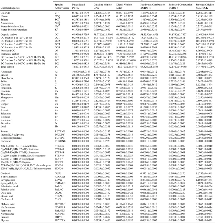
Table 1. Source profiles (percent of emitted PM2.5) used in CMB modeling for Fresno samples acquired during the CRPAQS winter intensive

study.

Source Type and Code

Species Paved Road Gasoline Vehicle Diesel Vehicle Hardwood Combustion Softwood Combustion Smoked Chicken Chemical Species Abbreviation PVRD GAS DIES BURN-H BURN-S SMCHICK Chloride Cl− _{0.1027±0.1839 0.4769±0.4318 0.2371±0.3495 1.4719±1.8146 0.1061±0.0323 1.2589±0.7814} Nitrate NO−₃ 0.0435±0.1817 1.6545±1.2115 0.1351±0.3835 0.6803±0.0567 0.1534±0.0293 0.4196±0.1199 Sulfate SO=₄ 0.2787±0.1881 6.7749±6.9651 3.5862±2.9797 1.4179±0.6204 0.5794±0.0597 0.4235±0.2699 Ammonium NH+₄ 0.3233±0.2305 3.0173±3.1377 1.1804±1.1875 0.4565±0.3963 0.2122±0.0312 0.1407±0.1188 Water-Soluble sodium Na+ _{0.0789±0.0351 0.0000±0.0010 0.0000±0.0010 0.3045±0.0252 0.1544±0.0117 0.2170±0.0291} Water-Soluble Potassium K+ _{0.1509±0.0899 0.0699±0.0682 0.1552±0.0529 2.9389±0.3286 0.8124±0.0594 0.3454±0.0354} Organic carbon OC 6.8950±3.7295 58.7720±21.5960 61.9970±24.9550 58.3350±4.6528 34.8740±2.7827 62.6800±9.5480 OC fraction 1 at 120◦_{C in He OC1 0.2746±0.2973 24.3710±18.1950 20.8160±7.6162 18.2440±5.3407 4.3149±0.3811 10.3330±4.9033} OC fraction 2 at 250◦C in He OC2 0.8838±0.6051 12.4740±4.9880 12.7670±6.2938 10.2400±1.2550 3.0070±0.3695 10.4480±2.4690 OC fraction 3 at 450◦_{C in He OC3 2.6704±1.3216 13.3020±6.0825 18.8010±7.2890 21.2100±3.4685 7.5739±0.6666 26.7180±12.7580} OC fraction 4 at 550◦_{C in He OC4 1.9571±0.8353 7.3284±2.8507 9.5810±5.4608 8.6300±1.2041 4.4939±0.6265 8.7359±1.2399} Pyrolized OC OP 1.1091±0.6952 1.2972±2.5596 0.0318±0.1382 0.0117±0.0399 15.4830±5.4853 5.7697±2.9909 Elemental carbon EC 0.9946±0.9520 28.5650±13.8100 78.3140±16.5500 5.1909±0.7901 27.2360±2.2356 11.8760±1.4911 EC fraction 1 at 550◦_{C in 98% He/2% O} 2 EC1 1.0781±0.7091 13.8680±6.1435 26.0500±5.9936 4.8393±0.9385 41.2150±3.0776 13.0800±3.1538

EC fraction 2 at 700◦C in 98% He/2% O2 EC2 1.0257±0.9381 15.5220±12.9970 51.9030±12.6890 0.3017±0.0576 1.3362±0.1858 3.9735±2.6549

EC fraction 3 at 800◦_{C in 98% He/2% O} 2 EC3 0.0000±0.0823 0.4739±0.3534 0.3886±0.3840 0.0606±0.0342 0.1676±0.0525 0.5915±0.5020 Total carbon TC 7.8897±4.6815 87.3370±25.6330 140.3100±29.9440 63.5260±5.0335 62.1100±4.9180 74.4750±10.7590 Aluminum Al 10.0008±3.0147 0.1073±0.0736 0.1717±0.1715 0.0944±0.0112 0.2013±0.0176 0.0508±0.0102 Silicon Si 28.1663±8.9603 4.7878±4.1119 1.2029±0.3647 0.2912±0.0230 1.0151±0.0724 0.5602±0.4483 Phosphorus P 0.3877±0.3543 0.3479±0.5129 0.1782±0.0555 0.0000±0.0073 0.0000±0.0057 0.0000±0.0061 Sulfur S 0.3516±0.2100 2.6670±2.4785 1.4845±1.1969 0.4240±0.0331 0.2352±0.0169 0.2427±0.0239 Chlorine Cl 0.1006±0.1422 0.2491±0.2978 0.0768±0.0424 1.3544±1.5612 0.1160±0.0090 1.6225±1.1894 Potassium K 2.8206±0.5488 0.0579±0.0474 0.1096±0.0910 2.9511±0.6782 1.0675±0.0758 0.5008±0.2895 Calcium Ca 3.4850±1.1771 0.7865±1.4028 0.7045±0.2820 0.1873±0.0225 0.5216±0.0376 0.1621±0.0436 Titantium Ti 0.4553±0.1348 0.0030±0.0569 0.0153±0.0914 0.0129±0.0197 0.0880±0.0096 0.0108±0.0287 Manganese Mn 0.0759±0.0054 0.0042±0.0042 0.0013±0.0066 0.0067±0.0007 0.0129±0.0011 0.0550±0.0049 Iron Fe 5.2254±1.0428 0.4226±0.3424 0.6570±0.4100 0.1402±0.0114 0.5172±0.0367 0.5990±0.5467 Copper Cu 0.0168±0.0119 0.0519±0.0537 0.0157±0.0066 0.0067±0.0006 0.0392±0.0028 0.0617±0.0067 Zinc Zn 0.0965±0.0467 0.4335±0.4056 0.3771±0.0872 0.1368±0.0135 0.0925±0.0066 0.0507±0.0049 Arsenic As 0.0016±0.0027 0.0001±0.0052 0.0004±0.0077 0.0007±0.0017 0.0006±0.0016 0.0019±0.0019 Selenium Se 0.0002±0.0010 0.0002±0.0027 0.0022±0.0041 0.0001±0.0007 0.0000±0.0007 0.0001±0.0009 Bromine Br 0.0016±0.0012 0.0375±0.0384 0.0451±0.0711 0.0045±0.0004 0.0014±0.0003 0.0166±0.0016 Rubidium Rb 0.0139±0.0046 0.0005±0.0022 0.0007±0.0038 0.0046±0.0005 0.0019±0.0003 0.0007±0.0011 Strontium Sr 0.0305±0.0016 0.0009±0.0023 0.0029±0.0039 0.0025±0.0004 0.0060±0.0006 0.0011±0.0011 Lead Pb 0.0109±0.0074 0.0257±0.0241 0.0086±0.0119 0.0039±0.0009 0.0030±0.0008 0.0082±0.0025 Retene RETENE 0.0000±0.0000 0.0042±0.0132 0.0002±0.0009 0.0272±0.0039 0.0140±0.0012 0.0059±0.0014 Indeno[123-cd]pyrene INCDPY 0.0000±0.0000 0.0340±0.0278 0.0000±0.0014 0.0028±0.0004 0.0033±0.0005 0.0053±0.0027 Benzo(ghi)perylene BGHIPE 0.0000±0.0000 0.0941±0.0827 0.0000±0.0017 0.0029±0.0008 0.0028±0.0008 0.0018±0.0035 Coronene CORONE 0.0000±0.0000 0.0836±0.0920 0.0000±0.0005 0.0011±0.0003 0.0008±0.0003 0.0001±0.0010 20S-13β(H),17α(H)-diacholestane STER35 0.0000±0.0000 0.0068±0.0060 0.0060±0.0036 0.0016±0.0005 0.0038±0.0009 0.0000±0.0010 C2920S-13β(H), 17α(H)-diasterane STER45 0.0000±0.0000 0.0182±0.0162 0.0040±0.0036 0.0001±0.0001 0.0000±0.0001 0.0000±0.0011 C2920S-13α(H), 17β(H)-diasterane STER48 0.0000±0.0000 0.0031±0.0037 0.0000±0.0009 0.0000±0.0001 0.0000±0.0001 0.0000±0.0010 C2820R-5α(H), 14α(H),17α(H)-ergostane STER49 0.0000±0.0000 0.0431±0.0978 0.0011±0.0027 0.0000±0.0001 0.0000±0.0001 0.0000±0.0010 17α(H), 21β(H)-29-Norhopane HOP17 0.0000±0.0000 0.0146±0.0262 0.0118±0.0075 0.0001±0.0002 0.0000±0.0001 0.0009±0.0011 17α(H), 21β(H)-29-Hopane HOP19 0.0000±0.0000 0.0446±0.0791 0.0062±0.0046 0.0006±0.0002 0.0008±0.0003 0.0026±0.0054 22S-17α(H),21β(H)-30,31,32-Trishomohopane HOP24 0.0000±0.0000 0.0026±0.0054 0.0000±0.0009 0.0005±0.0003 0.0005±0.0003 0.0000±0.0013 22R-17α(H),21β(H)-30,31,32-Trishomohopane HOP26 0.0000±0.0000 0.0025±0.0052 0.0000±0.0009 0.0001±0.0002 0.0001±0.0002 0.0001±0.0028 Guaiacol GUAI 0.0000±0.0000 0.0000±0.0000 0.0000±0.0000 0.3721±0.0309 0.2409±0.0170 1.6752±0.4991 4-allyl-guaiacol ALGUAI 0.0000±0.0000 0.0000±0.0027 0.0000±0.0006 0.1195±0.0085 0.0548±0.0055 0.0067±0.0067 Levoglucosan LEVG 0.0000±0.0000 0.0000±0.0120 0.0000±0.0175 2.2778±0.5924 0.1552±0.0172 1.1505±0.4381 Syringaldehyde SYRALD 0.0000±0.0000 0.0000±0.0000 0.0000±0.0000 0.4631±0.0307 0.0247±0.0017 0.1871±0.0224 Palmitoleic acid PALOL 0.0000±0.0000 0.0082±0.0117 0.0263±0.0217 0.0069±0.0005 0.0000±0.0002 0.0261±0.0234 Palmitic acid PALAC 0.0000±0.0000 0.0000±0.0486 0.0000±0.1507 0.0562±0.0041 0.0000±0.0323 0.0000±0.1940 Oleic acid OLAC 0.0000±0.0000 0.0000±0.0152 0.0000±0.0422 0.0652±0.0051 0.0000±0.0289 0.0000±0.1385 Stearic acid STEAC 0.0000±0.0000 0.0000±0.0173 0.0000±0.0358 0.0174±0.0013 0.0000±0.0289 0.0000±0.1574 Cholesterol CHOL 0.0000±0.0000 0.0000±0.0011 0.0000±0.0020 0.0000±0.0000 0.0000±0.0002 0.0003±0.0012 Phthalic acid PHTHAC 0.0000±0.0000 0.1026±0.2018 0.1864±0.1740 0.0141±0.0010 0.0000±0.0002 0.0065±0.0012 Norfarnesane NORFAR 0.0000±0.0000 0.0365±0.3020 0.0285±0.0236 0.0020±0.0010 0.0002±0.0002 0.0007±0.0014 Farnesane FARNES 0.0000±0.0000 0.0344±0.5172 0.0750±0.0914 0.0011±0.0008 0.0005±0.0005 0.0000±0.0012 Norpristance NORPRI 0.0000±0.0000 0.0422±0.3857 0.1178±0.0372 0.0006±0.0004 0.0000±0.0004 0.0025±0.0034 Pristane PRIST 0.0000±0.0000 0.0032±0.2887 0.0119±0.0145 0.0008±0.0005 0.0010±0.0004 0.0352±0.0086 Phytane PHYTAN 0.0000±0.0000 0.0139±0.4463 0.0974±0.0656 0.0015±0.0005 0.0004±0.0002 0.0041±0.0021

(AGRI), dairy and feed lot (CATTLE), lake deposits (SALT), and construction (CONST). OC and EC were measured in these samples but their specific organic compounds were not measured and they are set to zero in the profile.

Examination of the ambient data for sodium (Na) and chlorine (Cl) (sea salt markers) showed that Cl was de-pleted with respect to Na in pure sea salt, even at a coastal site like Bodega Bay where the average ratio of Cl/Na (for

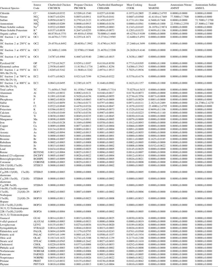
Table 1. Continued.

Source Type and Code

Source Charbroiled Chicken Propane Chicken Charbroiled Hamburger Meat Cooking Seasalt Ammonium Nitrate Ammonium Sulfate Chemical Species Code CHCHICK PRCHICK CHHAMB COOK MARINE AMNIT AMSUL Chloride Cl− 0.0449±0.0332 0.5209±0.1540 0.0257±0.0180 0.1972±0.2805 23.4880±2.6795 0.0000±0.0000 0.0000±0.0000 Nitrate NO−₃ 0.0637±0.0291 0.0855±0.0911 0.0570±0.0161 0.0687±0.0560 41.6110±4.7469 77.5000±7.7500 0.0000±0.0000 Sulfate SO= 4 0.0950±0.0672 0.2792±0.2123 0.1450±0.0377 0.1731±0.1304 6.5468±0.7468 0.0000±0.0000 72.7000±7.2700 Ammonium NH+₄ 0.0000±0.0289 0.0000±0.0915 0.0000±0.0156 0.0000±0.0561 0.0000±0.1000 22.5500±2.2550 27.3000±2.7300 Water-Soluble sodium Na+ _{0.0522±0.0069 0.2508±0.0264 0.0999±0.0083 0.1343±0.0165 26.1870±2.9874 0.0000±0.0000 0.0000±0.0000} Water-Soluble Potassium K+ 0.0157±0.0038 0.2647±0.0255 0.0804±0.0073 0.1203±0.0155 0.9699±0.1106 0.0000±0.0000 0.0000±0.0000 Organic carbon OC 68.8730±6.3751 69.4010±5.8564 70.0080±5.4660 69.4270±5.9109 0.0000±0.0000 0.0000±0.0000 0.0000±0.0000 OC fraction 1 at 120◦_{C in} He OC1 16.4470±3.7353 8.2255±8.1671 13.2710±2.9585 12.6480±5.4591 0.0000±0.0000 0.0000±0.0000 0.0000±0.0000 OC fraction 2 at 250◦_{C in} He OC2 29.4570±6.8492 20.6030±7.3992 31.6790±4.3935 27.2460±6.3499 0.0000±0.0000 0.0000±0.0000 0.0000±0.0000 OC fraction 3 at 450◦C in He OC3 18.3400±2.1696 32.9780±15.9640 21.4670±2.5208 24.2620±9.4146 0.0000±0.0000 0.0000±0.0000 0.0000±0.0000 OC fraction 4 at 550◦_{C in} He OC4 3.6787±0.4984 6.4667±0.9140 2.8861±0.4815 4.3438±1.8807 0.0000±0.0000 0.0000±0.0000 0.0000±0.0000 Pyrolized OC OP 0.7735±0.5627 0.9295±1.0107 0.6110±0.8550 0.7713±0.8305 0.0000±0.1000 0.0000±0.0000 0.0000±0.0000 Elemental carbon EC 2.5938±0.6693 11.8130±3.1734 2.4850±1.8256 5.6306±5.3543 0.0000±0.0000 0.0000±0.0000 0.0000±0.0000 EC fraction 1 at 550◦C in 98% He/2% O2 EC1 2.8265±0.5162 11.5840±4.3242 2.6974±1.0513 5.7025±5.0936 0.0000±0.0000 0.0000±0.0000 0.0000±0.0000 EC fraction 2 at 700◦_{C in} 98% He/2% O2 EC2 0.4571±0.0621 0.9213±0.7199 0.2344±0.0322 0.5376±0.4176 0.0000±0.0000 0.0000±0.0000 0.0000±0.0000 EC fraction 3 at 800◦_{C in} 98% He/2% O2 EC3 0.0843±0.0495 0.2385±0.1675 0.1640±0.0982 0.1623±0.1157 0.0000±0.1000 0.0000±0.0000 0.0000±0.0000 Total carbon TC 71.4450±5.7045 81.1550±7.9406 72.4800±5.7314 75.0270±6.5433 0.0000±0.0000 0.0000±0.0000 0.0000±0.0000 Aluminum Al 0.0291±0.0032 0.0082±0.0121 0.0160±0.0017 0.0178±0.0073 0.0000±0.0000 0.0000±0.0000 0.0000±0.0000 Silicon Si 0.1891±0.0160 0.5620±0.6156 0.0698±0.0055 0.2736±0.3556 0.0073±0.0008 0.0000±0.0000 0.0000±0.0000 Phosphorus P 0.0002±0.0026 0.0083±0.0043 0.0074±0.0009 0.0053±0.0029 0.0001±0.0000 0.0000±0.0000 0.0000±0.0000 Sulfur S 0.0532±0.0059 0.1584±0.0173 0.0797±0.0061 0.0971±0.0111 2.1823±0.2489 0.0000±0.0000 24.2700±2.4270 Chlorine Cl 0.0522±0.0040 0.4478±0.0326 0.0636±0.0047 0.1879±0.0192 23.4880±2.6795 0.0000±0.0000 0.0000±0.0000 Potassium K 0.0386±0.0032 0.3212±0.0236 0.0990±0.0073 0.1529±0.0144 0.9699±0.1106 0.0000±0.0000 0.0000±0.0000 Calcium Ca 0.1658±0.0169 0.0783±0.0336 0.0987±0.0091 0.1143±0.0223 0.9990±0.1140 0.0000±0.0000 0.0000±0.0000 Titantium Ti 0.0030±0.0083 0.0049±0.0235 0.0011±0.0045 0.0030±0.0146 0.0000±0.0000 0.0000±0.0000 0.0000±0.0000 Manganese Mn 0.0098±0.0009 0.0074±0.0011 0.0066±0.0005 0.0079±0.0009 0.0000±0.0000 0.0000±0.0000 0.0000±0.0000 Iron Fe 0.1430±0.0128 0.1049±0.0090 0.0558±0.0041 0.1012±0.0093 0.0000±0.0000 0.0000±0.0000 0.0000±0.0000 Copper Cu 0.0089±0.0008 0.0077±0.0013 0.0033±0.0004 0.0066±0.0009 0.0000±0.0000 0.0000±0.0000 0.0000±0.0000 Zinc Zn 0.0134±0.0010 0.0089±0.0011 0.0051±0.0004 0.0091±0.0009 0.0000±0.0000 0.0000±0.0000 0.0000±0.0000 Arsenic As 0.0002±0.0094 0.0002±0.0015 0.0001±0.0003 0.0002±0.0055 0.0000±0.0000 0.0000±0.0000 0.0000±0.0000 Selenium Se 0.0000±0.0003 0.0001±0.0006 0.0000±0.0001 0.0000±0.0004 0.0000±0.0000 0.0000±0.0000 0.0000±0.0000 Bromine Br 0.0006±0.0007 0.0018±0.0005 0.0010±0.0001 0.0011±0.0005 0.1625±0.0185 0.0000±0.0000 0.0000±0.0000 Rubidium Rb 0.0002±0.0003 0.0005±0.0008 0.0000±0.0002 0.0002±0.0005 0.0000±0.0000 0.0000±0.0000 0.0000±0.0000 Strontium Sr 0.0015±0.0003 0.0004±0.0010 0.0006±0.0002 0.0008±0.0006 0.0192±0.0022 0.0000±0.0000 0.0000±0.0000 Lead Pb 0.0434±0.0044 0.0000±0.0025 0.0000±0.0005 0.0145±0.0029 0.0000±0.0000 0.0000±0.0000 0.0000±0.0000 Retene RETENE 0.0012±0.0004 0.0025±0.0012 0.0006±0.0002 0.0014±0.0007 0.0000±0.0000 0.0000±0.0000 0.0000±0.0000 Indeno[123-cd]pyrene INCDPY 0.0005±0.0007 0.0028±0.0022 0.0003±0.0004 0.0012±0.0014 0.0000±0.0000 0.0000±0.0000 0.0000±0.0000 Benzo(ghi)perylene BGHIPE 0.0003±0.0009 0.0068±0.0034 0.0008±0.0005 0.0026±0.0021 0.0000±0.0000 0.0000±0.0000 0.0000±0.0000 Coronene CORONE 0.0000±0.0003 0.0029±0.0013 0.0000±0.0002 0.0010±0.0008 0.0000±0.0000 0.0000±0.0000 0.0000±0.0000 20S-13β(H),17α(H)-diacholestane STER35 0.0000±0.0003 0.0000±0.0008 0.0000±0.0002 0.0000±0.0005 0.0000±0.0000 0.0000±0.0000 0.0000±0.0000 C2920S-13β(H), 17α(H)-diasterane STER45 0.0000±0.0003 0.0000±0.0008 0.0000±0.0002 0.0000±0.0005 0.0000±0.0000 0.0000±0.0000 0.0000±0.0000 C2920S-13α(H), 17β(H)-diasterane STER48 0.0000±0.0003 0.0000±0.0008 0.0000±0.0002 0.0000±0.0005 0.0000±0.0000 0.0000±0.0000 0.0000±0.0000 C2820R-5α(H), 14α(H),17α(H)-ergostane STER49 0.0000±0.0003 0.0000±0.0008 0.0001±0.0002 0.0000±0.0005 0.0000±0.0000 0.0000±0.0000 0.0000±0.0000 17α(H), 21β(H)-29-Norhopane HOP17 0.0002±0.0003 0.0007±0.0009 0.0001±0.0002 0.0003±0.0006 0.0000±0.0000 0.0000±0.0000 0.0000±0.0000 17α(H), 21β(H)-29-Hopane HOP19 0.0000±0.0011 0.0000±0.0023 0.0003±0.0008 0.0001±0.0015 0.0000±0.0000 0.0000±0.0000 0.0000±0.0000 22S-17α(H),21β(H)-30,31,32-Trishomohopane HOP24 0.0000±0.0004 0.0000±0.0008 0.0000±0.0002 0.0000±0.0005 0.0000±0.0000 0.0000±0.0000 0.0000±0.0000 22R-17α(H),21β(H)-30,31,32-Trishomohopane HOP26 0.0000±0.0004 0.0000±0.0008 0.0000±0.0002 0.0000±0.0005 0.0000±0.0000 0.0000±0.0000 0.0000±0.0000 Guaiacol GUAI 0.0014±0.0013 0.0015±0.0026 0.0060±0.0025 0.0030±0.0026 0.0000±0.0000 0.0000±0.0000 0.0000±0.0000 4-allyl-guaiacol ALGUAI 0.0000±0.0003 0.0000±0.0033 0.0000±0.0006 0.0000±0.0019 0.0000±0.0000 0.0000±0.0000 0.0000±0.0000 Levoglucosan LEVG 0.0135±0.0017 0.0274±0.0036 0.0159±0.0020 0.0189±0.0026 0.0000±0.0000 0.0000±0.0000 0.0000±0.0000 Syringaldehyde SYRALD 0.0016±0.0004 0.0046±0.0010 0.0015±0.0003 0.0026±0.0018 0.0000±0.0000 0.0000±0.0000 0.0000±0.0000 Palmitoleic acid PALOL 0.0694±0.0499 0.1179±0.0795 0.0410±0.0243 0.0761±0.0560 0.0000±0.0000 0.0000±0.0000 0.0000±0.0000 Palmitic acid PALAC 0.0593±0.1499 0.0001±0.2811 0.0508±0.1037 0.0367±0.1934 0.0000±0.0000 0.0000±0.0000 0.0000±0.0000 Oleic acid OLAC 0.1813±0.1632 0.2741±0.3188 0.1965±0.1239 0.2173±0.2188 0.0000±0.0000 0.0000±0.0000 0.0000±0.0000 Stearic acid STEAC 0.0000±0.0565 0.0000±0.2642 0.0027±0.0693 0.0009±0.1610 0.0000±0.0000 0.0000±0.0000 0.0000±0.0000 Cholesterol CHOL 0.0220±0.0058 0.0373±0.0088 0.0283±0.0053 0.0292±0.0068 0.0000±0.0000 0.0000±0.0000 0.0000±0.0000 Phthalic acid PHTHAC 0.0009±0.0003 0.0078±0.0013 0.0000±0.0002 0.0029±0.0008 0.0000±0.0000 0.0000±0.0000 0.0000±0.0000 Norfarnesane NORFAR 0.0000±0.0003 0.0000±0.0008 0.0000±0.0002 0.0000±0.0005 0.0000±0.0000 0.0000±0.0000 0.0000±0.0000 Farnesane FARNES 0.0000±0.0003 0.0000±0.0008 0.0003±0.0004 0.0001±0.0005 0.0000±0.0000 0.0000±0.0000 0.0000±0.0000 Norpristance NORPRI 0.0059±0.0018 0.0010±0.0026 0.0112±0.0022 0.0060±0.0022 0.0000±0.0000 0.0000±0.0000 0.0000±0.0000 Pristane PRIST 0.0112±0.0032 0.0135±0.0043 0.0238±0.0048 0.0162±0.0042 0.0000±0.0000 0.0000±0.0000 0.0000±0.0000 Phytane PHYTAN 0.0018±0.0006 0.0001±0.0013 0.0012±0.0004 0.0010±0.0009 0.0000±0.0000 0.0000±0.0000 0.0000±0.0000

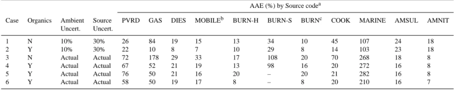
Table 2. Average absolute error (AAE %) between the CMB estimated and true source contribution estimates from simulated data.

AAE (%) by Source codea

Case Organics Ambient Source PVRD GAS DIES MOBILEb BURN-H BURN-S BURNc COOK MARINE AMSUL AMNIT Uncert. Uncert. 1 N 10% 30% 26 84 19 15 13 34 10 45 107 24 18 2 Y 10% 30% 22 10 8 7 10 29 8 14 103 23 18 3 N Actual Actual 72 178 29 33 17 108 20 70 268 18 8 4 Y Actual Actual 67 52 21 19 13 98 16 20 272 16 8 5 Y Actual Actual 76 50 21 16 20 – 20 21 282 16 8 6 Y Actual Actual 58 50 19 17 8 – 8 20 210 16 7

a_{See Table 1 for source codes} b_{MOBILE=GAS+DIES} c_{BURN=BURN-H+BURN-S}

Case 1: Data generated with BURN-H (hardwood) and BURN-S (softwood), no organics in CMB. Case 2: Data generated with BURN-H (hardwood) and BURN-S (softwood), organics in CMB. Case 3: Data generated with BURN-H (hardwood) and BURN-S (softwood), no organics in CMB. Case 4: Data generated with BURN-H (hardwood) and BURN-S (softwood), organics in CMB.

Case 5: Data generated with BURN-H (hardwood) and BURN-S (softwood), organics in CMB, no BURN-S in CMB. Case 6: Data generated with BURN-H (hardwood) only, organics in CMB.

concentrations greater than their uncertainties) was 1.1 com-pared with a pure sea salt ratio of 1.8. This depletion re-sults from reactions of sea salt particles with strong acids like HNO3, where NO−₃ substitutes for Cl (Mamane and Gottlieb, 1992). To account for this, a “reacted” sea salt profile (MA-RINE) was used in which half of the Cl was replaced by NO−₃ on a molar basis (Chow et al., 1996). Secondary NO−₃ and SO=₄ were represented by pure ammonium nitrate (AMNIT; NH4NO3) and ammonium sulfate [AMSUL; (NH4)2SO4] profiles, respectively.

3 Results and discussion 3.1 CMB feasibility analysis

Simulated data were generated with methods described by Javitz et al. (1988), Lowenthal et al. (1992), and Chow et al. (2004b). Average true source contributions from PVRD, GAS, DIES, BURN-H, BURN-S, COOK, MARINE, AM-SUL, and AMNIT of 1, 3, 10, 30, 10, 10, 0.1, 5, and 30 µg/m3, respectively, were based on previous SJV source apportionments studies. True Sj t were created by randomly perturbing the average values (above) with a coefficient of variation (CV) of 50%, assuming a lognormal distribution. Synthetic concentrations were calculated for each “sample” using Eq. (1). Random lognormal variation for the source profiles (F) and measurement uncertainty was introduced to the derived concentrations (C) in two ways: 1) assuming measurement uncertainty and source profile variations of 10 and 30%, respectively; and 2) using the root-mean squared uncertainties of ambient concentrations and the actual stan-dard deviations of the composite source profiles. The lat-ter approach may be more realistic because some species

are measured more precisely than others. Cholesterol lev-els were below lower quantifiable limits (LQLs) in many of the samples owing to the short sample durations and periods of the day when cooking contributions were not expected. Cholesterol has also been reported to react with ozone un-der ambient conditions (Dreyfus et al., 2005). However, cholesterol was well-determined in the meat cooking emis-sions samples. To allow this compound to act as a useful marker for cooking in the simulations, its uncertainty in the ambient measurements was assumed to be 10%.

The CMB model was applied to the two data sets, each with 100 simulated samples using the average source profiles with weighting based on the uncertainties described above. The variance of the Sj t is the precision attainable for a par-ticular source mix for a model with specified random er-rors. This precision is expressed as the average absolute error (AAE %), which is the average (N=100) of the absolute per-cent differences between the estimated and true Sj t. Results are summarized in Table 2.

Case 1 represents fixed uncertainty without organics. The

SMARINE AAE was large (107%) because the true aver-age SMARINE was only 0.1 µg/m3. The AAEs for SDIES and SBURN−H were less than 20% while the AAEs for

SGAS, SBURN−S, and SCOOK were 84, 34 and 45%, respec-tively. When organics were included (Case 2), the AAEs were much lower for SGAS, SDIES, and SCOOK, but they did not change as much for SBURN−H and SBURN−S. In-cluding organic compounds reduced collinearity (similar-ity) among profiles for the vehicle exhaust and cooking sources. Except for SBURN−H, SAMSUL, and SAMNIT, the AAEs for Case 3 (no organics) were considerably larger than for Case 1: 72, 178, 29, 108, 70, and 268% for con-tributions from PVRD, GAS, DIES, BURN-S, COOK, and

MARINE, respectively. Including organics (Case 4) reduced the SGAS, SDIES, SBURN−H, and SCOOKAAEs to 52, 21, 13, and 20%, respectively. While the SBURN−H AAE improved somewhat (from 17% to 13%) when organics were included, the SBURN−SAAE remained high (98%).

These results verify that organic markers can help distin-guish contributions from gasoline exhaust, diesel exhaust, and cooking by increasing the differences between their source profiles. However, organics were not needed to es-timate the wood burning contribution. Organics did not appear to separate hardwood and softwood contributions, even though there are noticeable differences between their source profiles. For example, the OC, EC, K+, levoglucosan, 4-allyl-guaiacol, and syringaldehyde compositions of hard-wood smoke were 58, 5.2, 2.9, 2.3, 0.12, and 0.46%, respec-tively, compared with 35, 27, 0.81, 0.16, 0.055, and 0.025%, respectively, for softwood smoke. Case 5 demonstrates the collinearity between the hardwood and softwood profiles by removing BURN-S from the CMB fit. Even though softwood combustion emissions contributed to the simulated concen-trations, the hardwood profile (BURN-H) was sufficient to estimate the total burning contribution to within 20%. When all of the actual burning contribution came from hardwood combustion, the SBURN−HAAE was only 8%.

The CMB8 model output contains the diagnostic MPIN (modified pseudo-inverse normalized) matrix (Kim and Henry, 1999). The MPIN identifies the influence of the fitting species on the source contribution estimates. An MPIN value of one indicates the highest influence. Aver-age concentrations from Case 4, Table 2 were subjected to CMB analysis and the MPIN was calculated. The influential species in the source profiles were as expected: Al and Si for PVRD (paved road); benzo(ghi)perylene, coronene, and indeno[123-cd]pyrene for gasoline vehicles; the EC2 ther-mal fraction for diesel vehicles; K+, levoglucosan, and sy-ringaldehyde for hardwood combustion; EC for softwood combustion; and cholesterol for cooking.

These tests with simulated data demonstrate the feasibility of identifying and quantifying gasoline- and diesel-exhaust contributions with reasonable precision using organic mark-ers. This is also the case for cooking contributions. Organics were not necessary to estimate the RWC contribution and it was not feasible to distinguish hardwood and softwood con-tributions from the source profiles used in this study, even when organics were included in the CMB model.

3.2 Initial source contribution estimates

Following the CMB applications and validation protocol (Watson et al., 1998b), the stability of the Sj t to different selections of source profiles and fitting species was evalu-ated for the average concentrations for the 00:00–05:00 PST sampling period. Ambient concentrations during this inter-val, including those of levoglucosan and cholesterol, mark-ers for RWC and cooking, respectively, were relatively high

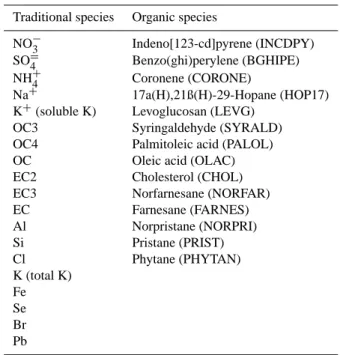
Table 3. Fitting speciesaused in CMB modeling for Fresno winter intensive samples.

Traditional species Organic species

NO−₃ Indeno[123-cd]pyrene (INCDPY) SO=₄ Benzo(ghi)perylene (BGHIPE) NH+₄ Coronene (CORONE)

Na+ 17a(H),21ß(H)-29-Hopane (HOP17) K+(soluble K) Levoglucosan (LEVG)

OC3 Syringaldehyde (SYRALD) OC4 Palmitoleic acid (PALOL) OC Oleic acid (OLAC) EC2 Cholesterol (CHOL) EC3 Norfarnesane (NORFAR) EC Farnesane (FARNES) Al Norpristane (NORPRI) Si Pristane (PRIST) Cl Phytane (PHYTAN) K (total K) Fe Se Br Pb

a_{See Table 1 for chemical species.}

and it is expected that this period is not dominated by a sin-gle source contribution. Chemical species whose concen-trations were less than their uncertainties in most samples (more than 40 out of 51 total sampling periods in Fresno) were not included in the CMB model. While cholesterol did not fit this criterion, it was included because of its potential value as a cooking marker. Initial model runs indicated that other species were not adequately accounted for in the CMB. Calcium (Ca), whose concentrations were greater than twice their uncertainties in only 15 out of 51 samples, was overes-timated by a factor of 5. Copper (Cu) and zinc (Zn) could not be explained by the available source profiles, including mu-nicipal incineration and brake wear. These species may be enriched by exhaust from the sampling equipment (Hoffman and Duce, 1971; King and Toma, 1975; Patterson, 1980). Guaiacol and 4-allyl-guaiacol, potential RWC markers, were underestimated by factors of 2 to 10. This could be attributed to differences between the profile fuels and burning condi-tions and those used in Fresno. Thermal carbon fraccondi-tions were included except for OP (pyrolized OC), OC1 and OC2, which are believed to contain much of the adsorbed organic vapors on quartz filters, and EC1, which may contain some pyrolysis products. Table 3 shows the 19 traditional and 14 organic species included in subsequent CMB analyses.

Case 1 in Table 4 gives the CMB solution for the “best fit”, which included organic species and both hardwood and softwood RWC source profiles. In a statistical sense, it is not clear that the BURN-S contribution was resolved because its

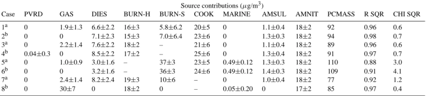
Table 4. Source contribution estimates from the CMB trial runs for average Fresno winter intensive samples during the early morning (00:00–05:00 PST) period, with and without organics for various source mixes.

Source contributions (µg/m3)

Case PVRD GAS DIES BURN-H BURN-S COOK MARINE AMSUL AMNIT PCMASS R SQR CHI SQR 1a 0 1.9±1.3 6.6±2.2 16±3 5.8±6.2 20±5 0 1.1±0.4 18±2 92 0.96 0.6 2b 0 0 7.1±2.3 15±3 7.0±6.4 23±6 0 1.3±0.3 18±2 94 0.98 0.7 3a 0 2.2±1.4 7.6±2.2 18±2 – 21±6 0 1.1±0.4 18±2 89 0.96 0.6 4b 0.04±0.3 0 8.5±2.2 17±2 – 25±6 0 1.3±0.4 18±2 91 0.97 0.7 5a 0 1.0±0.9 3.0±1.6 – 37±3 23±5 0.49±0.12 1.3±0.3 18±2 110 0.88 3.0 6b 0 0 3.2±1.6 – 36±3 24±6 0.49±0.12 1.4±0.3 18±2 109 0.91 4.1 7a 0 2.4±1.4 8.2±2.4 19±3 10±6 – 0 1.0±0.4 18±2 77 0.92 1.2 8b 0 30±7 0 18±2 0 – 0.05±0.20 0 17±2 85 0.97 0.4 a_{With organics.} b_{Without organics.}

value was lower than its uncertainty. On the other hand, in-cluding this source accounted for a larger percentage of the measured mass. The best estimate of the RWC contribution may be the sum of SBURN−H and SBURN−S(22±7 µg/m3). Similarly, while GAS and DIES contributions were resolved, the uncertainty of SGAS (1.9±1.3 µg/m3)was large (68%). The cooking contribution was large (20±5 µg/m3)as was the secondary NH4NO3 contribution (18±2 µg/m3). Zero val-ues for SPVRDand SMARINEindicate that their contributions became negative in the iterative solution and that their re-spective source profiles were dropped from the model. Most of the measured mass was accounted for (PCMASS=92) and the included sources explained the ambient chemical concen-trations well (R SQR=0.96, CHI SQR=0.6).

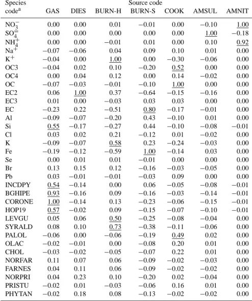
The distinguishing chemical markers for the sources in Case 1 were examined with the MPIN matrix, a feature of the CMB8 model, shown in Table 5. According to the MPIN, the most important markers for cooking were OC, OC3, and palmitoleic acid. Cholesterol exhibited a relatively low value because its average ambient concentration was smaller than its uncertainty. The MPIN indicated that the most impor-tant GAS markers were coronene and benzo(ghi)perylene, as expected. The EC2 fraction was the most important DIES marker. The principal hardwood (BURN-H) markers were K+and syringaldehyde. Levoglucosan was also an impor-tant marker with a value of 0.5. The MPIN shows that the most influential marker for softwood (BURN-S) was Fe, but this should not be the case.

Case 2 (Table 4) was the same as Case 1 except that or-ganic species were excluded from the fit. Except for a SGAS of zero, the solution was very similar to Case 1 (with organ-ics) although SCOOKwas 3 µg/m3higher. Cases 3 and 4 were analogous to Cases 1 and 2, respectively, except that BURN-S was removed from the model. In Case 3, with organics, removing BURN-S increased the SGAS and SDIES slightly and increased SBURN−H and SCOOK by 2 and 1 µg/m3, re-spectively. In Case 4 (without organics), all of the vehicle

exhaust contribution was assigned to DIES, as in Case 2, and

SCOOK increased from 23±6 (Case 2) to 25±6 µg/m3. Re-moving BURN-S in Cases 3 and 4 reduced PCMASS by 3% and most of this decrease came from the burning source con-tribution.

Case 5 (with organics) and Case 6 (without organics) were analogous to Cases 3 and 4, respectively, except that BURN-S was included and BURN-H was excluded from the model. This caused a large increase in the burning contribution, to 37±3 and 36±3 µg/m3, with and without organics, respec-tively, and an overestimation of measured mass by 10 and 9%, respectively. Both SGAS and SDIES were reduced by about a factor of 2 and SCOOK increased by 3 µg/m3 com-pared with Case 1. The R SQR decreased and CHI SQR increased dramatically compared with previous cases, indi-cating that BURN-S did not explain the traditional or organic species concentrations as well as BURN-H.

Finally, the cooking profile was removed while BURN-H and BURN-S were retained. In Case 7 (with organics), the solution was similar to that of Case 1 although SGAS and SDIES increased somewhat while the total burning con-tribution increased from 22±7 to 29±7 µg/m3. The solu-tion changed dramatically without organics (Case 8). All of

SBURN−Sand SCOOKwere assigned to SGAS(30±7 µg/m3). Both DIES and BURN-S were eliminated from the fit. Note that while mass was underestimated by 15%, this model fit the non-organic concentrations well (R SQR=0.97, CHI SQR=0.4). However, the previous results suggest that this solution was not realistic and that cooking should be included in the model, even though its uncertainty is large.

The solutions for Cases 1 through 4 were relatively stable with or without organics. Gasoline and diesel contributions were not resolved without organics. The overall burning con-tribution (hardwood plus softwood) depended mainly on K+ and not on organics. The cooking contribution was most influenced by OC and OC3, probably because cholesterol was lower than LQLs in most samples. However, when the

Table 5. Modified pseudo-inverse normalized (MPIN) matrix in the CMB model for Case 1 of Table 4. Key species for each source are underlined.

Species Source code

codea GAS DIES BURN-H BURN-S COOK AMSUL AMNIT NO−₃ 0.00 0.00 0.01 −0.01 0.00 −0.10 1.00 SO=₄ 0.00 0.00 0.00 0.00 0.00 1.00 −0.18 NH+₄ 0.00 0.00 −0.01 0.01 0.00 0.10 0.92 Na+ −0.07 −0.06 0.04 0.09 0.10 0.01 0.00 K+ −0.04 0.00 1.00 0.00 −0.30 −0.06 0.00 OC3 −0.04 0.02 0.10 −0.20 0.52 0.00 0.00 OC4 0.00 0.04 0.12 0.00 0.14 −0.02 0.00 OC −0.07 −0.03 −0.01 −0.10 1.00 0.00 0.00 EC2 0.06 1.00 0.37 −0.64 −0.15 −0.16 0.00 EC3 0.01 0.00 −0.03 0.03 0.03 0.00 0.00 EC −0.23 0.22 −0.51 0.80 −0.17 −0.01 0.00 Al −0.09 −0.07 −0.20 0.43 −0.10 0.01 0.00 Si 0.55 −0.17 −0.27 0.44 −0.10 −0.08 −0.01 Cl 0.03 0.02 0.21 −0.12 0.01 −0.02 0.00 K −0.09 −0.07 0.58 0.23 −0.24 −0.03 0.00 Fe −0.19 −0.12 −0.59 1.00 −0.14 0.03 0.00 Se 0.00 0.01 0.01 −0.01 0.00 0.00 0.00 Br 0.13 0.15 0.12 −0.16 −0.03 −0.05 0.00 Pb 0.03 −0.01 −0.01 −0.03 0.09 0.00 0.00 INCDPY 0.54 −0.14 0.00 0.06 −0.05 −0.08 −0.01 BGHIPE 0.93 −0.16 0.09 −0.16 −0.03 −0.14 −0.01 CORONE 1.00 −0.14 0.13 −0.23 −0.06 −0.15 −0.01 HOP19 0.57 −0.02 0.09 −0.15 −0.07 −0.10 −0.01 LEVGU 0.05 0.06 0.50 −0.25 −0.08 −0.04 0.00 SYRALD 0.08 0.10 0.73 −0.38 −0.11 −0.06 0.00 PALOL −0.06 0.00 −0.06 −0.19 0.49 0.02 0.00 OLAC −0.02 −0.01 0.00 −0.08 0.20 0.01 0.00 CHOL −0.03 −0.02 −0.05 −0.07 0.22 0.01 0.00 NORFAR 0.11 0.07 0.06 −0.09 −0.02 −0.03 0.00 FARNES 0.04 0.11 0.06 −0.09 −0.02 −0.02 0.00 NORPRI 0.04 0.23 0.10 −0.20 0.02 −0.04 0.00 PRISTU −0.02 0.01 −0.03 −0.06 0.16 0.01 0.00 PHYTAN −0.02 0.18 0.08 −0.13 −0.02 −0.02 0.00

a_{See Table 1 for chemical species.}

cholesterol uncertainty was reduced to 10% of the average concentration, the solution remained similar to that of Case 1, even though cholesterol became the most influential marker for cooking according to the MPIN. The cooking contribu-tion is highly uncertain.

3.3 Source apportionment during winter (2000–2001) in Fresno

Each of the 51 samples collected in Fresno was subjected to CMB analysis. The average r2, chi-square, and percent mass accounted for were 0.89, 1.78, and 92%, respectively, when organics were included in the CMB and 0.92, 1.23, and 104%, respectively, without organics. Organics did not fit as well as traditional species, but including organics

ac-counted for more of the measured mass. Table 6 presents average source contribution estimates (from CMB including organics) based on: 1) the duration-weighted average of the CMB results from the 51 individual samples (Case A); 2) the average of the CMB results from the four intensive periods (Case B); and 3) the CMB result of the duration-weighted av-erage concentrations of the 51 individual samples (Case C). The species in Table 3 were included and CMB8 was run in “auto fit” mode using the “s. elim.” option to constrain the source contribution estimates to positive values.

In all cases, PVRD was not detected. GAS was larger than DIES in Cases A and B, although they were equiva-lent within stated uncertainty levels. The combined vehicle exhaust contributions were 14 and 15% of measured PM2.5. For Case C (average sample), DIES (4.7 µg/m3)was more

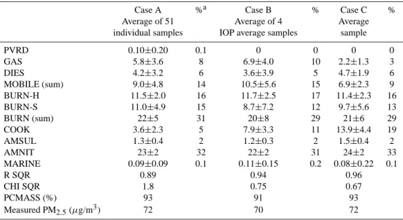
Table 6. CMB source contribution estimates (µg/m3)for the CRPAQS winter intensive samples in Fresno.

Case A %a Case B % Case C % Average of 51 Average of 4 Average individual samples IOP average samples sample

PVRD 0.10±0.20 0.1 0 0 0 0 GAS 5.8±3.6 8 6.9±4.0 10 2.2±1.3 3 DIES 4.2±3.2 6 3.6±3.9 5 4.7±1.9 6 MOBILE (sum) 9.0±4.8 14 10.5±5.6 15 6.9±2.3 9 BURN-H 11.5±2.0 16 11.7±2.5 17 11.4±2.3 16 BURN-S 11.0±4.9 15 8.7±7.2 12 9.7±5.6 13 BURN (sum) 22±5 31 20±8 29 21±6 29 COOK 3.6±2.3 5 7.9±3.3 11 13.9±4.4 19 AMSUL 1.3±0.4 2 1.2±0.3 2 1.5±0.4 2 AMNIT 23±2 32 22±2 31 24±2 33 MARINE 0.09±0.09 0.1 0.11±0.15 0.2 0.08±0.22 0.1 R SQR 0.89 0.94 0.96 CHI SQR 1.8 0.75 0.67 PCMASS (%) 93 91 93 Measured PM2.5(µg/m3) 72 70 72 a_{Percent of measured PM} 2.5. Start Hour PST 0 5 10 16 P e rce n t o f Es ti ma te d P M2 .5 0 20 40 60 80 MOBILE (GAS+DIES) RWC (BURN-H+BURN-S) COOK AMNIT

Fig. 1. Average diurnal variation of source contributions (percent of estimated PM_2.5)for mobile (MOBILE = GAS + DIES), resi-dential wood combustion (RWC = BURN-H + BURN-S), cooking (COOK), and secondary ammonium nitrate (AMNIT) during the CRPAQS winter intensive study at the Fresno Supersite in Califor-nia. The values represent averages from the four sample periods, 00:00–05:00, 05:00–10:00, 10:00–16:00, and 16:00–24:00 PST.

than twice GAS (2.2 µg/m3). The combined vehicle ex-haust contribution was 9% of measured PM2.5. BURN-H was 16–17% in all cases, averaging 11.5 µg/m3. BURN-S ranged from 12–15% although its uncertainty was large, es-pecially in Cases B and C. BURN-H and BURN-S combined ranged from 20 µg/m3 for Case B (29%) to 22 µg/m3 for Case A (31%). COOK was the most variable, ranging from

3.6 µg/m3 (5% of PM2.5)for Case A to 13.9 µg/m3 (19% of PM2.5)for Case C. AMSUL ranged from 1.2–1.5 µg/m3 (2% of PM2.5), while AMNIT (22–24 µg/m3), accounted for 31–33% of PM2.5. The MARINE contribution was not sig-nificant in any of the cases. Overall, PM2.5mass was under-estimated by less than 10%. The CMB performance mea-sures were better for average samples (Cases B and C) than for individual samples (Case A).

Average diurnal variations of source contributions are pre-sented in Fig. 1. Average source contributions derived from CMB analysis, including organics, from mobile (MOBILE = GAS + DEISEL), residential wood combustion (RWC = BURN-H + BURN-S), cooking (COOK), and secondary am-monium nitrate (AMNIT) for the 00:00–05:00, 05:00–10:00, 10:00–16:00, and 16:00–24:00 PST periods were calculated as a percentage of total estimated PM2.5 mass. AMNIT in-creased in the afternoon period (10:00–16:00 PST) as trans-ported pollutants were mixed to the surface (Watson and Chow, 2002; Chow et al., 2006a). Cooking and burning con-tributions displayed similar diurnal variations, with the high-est relative contributions in the evening (16:00–24:00 PST) and early morning hours (00:00–05:00 PST). The mobile contribution varied least during the day although the percent contributions were highest in the evening and mid-morning (05:00–10:00) periods. Watson et al. (2002b, 2006b) drew similar conclusions about diurnal variations of source contri-butions in Fresno from continuous measurements of particle size distributions and NOx, CO, and black carbon concentra-tions.

Ambient Water-Soluble K (μg/m3) 0.1 0.2 0.3 0.4 0.5 0.6 R W C C o n tri b u ti o n (μ g /m 3 ) 0 5 10 15 20 25 30 35 40

Ambient Palmitoleic Acid (μg/m3)

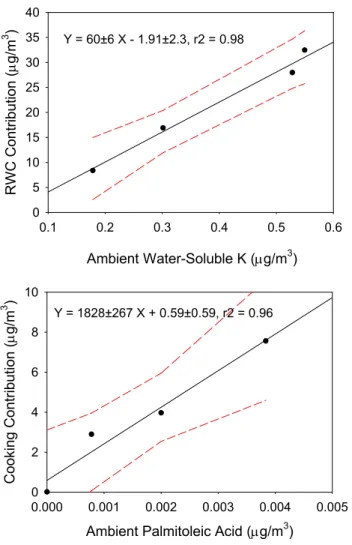
0.000 0.001 0.002 0.003 0.004 0.005 C o o k in g C o n tri b u ti o n (μ g /m 3 ) 0 2 4 6 8 10 Y = 60±6 X - 1.91±2.3, r2 = 0.98 Y = 1828±267 X + 0.59±0.59, r2 = 0.96

Fig. 2. Comparison of average residential wood combustion (RWC) and cooking contributions and average ambient water-soluble potas-sium (K+) and palmitoleic acid concentrations during four CR-PAQS winter intensive periods at the Fresno Supersite in California. The values represent averages from the four sample periods dur-ing the winter intensive study (00:00–05:00, 05:00–10:00, 10:00– 16:00, and 16:00–24:00 PST). Included in the figure are the regres-sion parameters and the 95% confidence interval of the expected values of the dependent variable.

While deviations between the measured source profiles and the composition of actual emissions near the Fresno Su-persite are probably the largest source of uncertainty, it is dif-ficult to assess the magnitude of these errors. Applying the source profiles to simulated data defines expected estimation error under ideal conditions where such errors are random. CMB analysis of ambient concentrations averaged on vari-ous time scales provides bounds on source contribution esti-mates under real-world conditions. Reported cholesterol and palmitoleic acid concentrations were larger than their mea-surement uncertainties for only 12 and 25%, respectively, of the Fresno samples. The inability to detect cooking markers probably contributed to large uncertainties for the estimated

Table 7. Fresno source contributions (%) from CMB during IMS95 (Schauer and Cass, 2000) and CRPAQS winter intensive study. Also shown are contributions from the California emission inven-tory (CARB, 2004).

Source IMS95a CRPAQSb SJV Emission Inventoryc Paved road dust 0 0 22 Vehicle exhaust (gasoline) 3 7 – Vehicle exhaust (diesel) 10 6 – Vehicle exhaust (combined) 13 13 8

Wood burning 41 30 11

Cooking 8 12 2

Secondary ammonium sulfate 4 2 – Secondary ammonium nitrate 30 32 –

Marine – 0 –

a_{Percent of estimated PM} 2.5mass. b_{Percent of measured PM}

2.5mass.

c_{Renormalized to include secondary ammonium sulfate and}

am-monium nitrate.

cooking contribution, i.e., from 5 to 19% of PM2.5. On the other hand, the total RWC contribution was stable.

Figure 2 shows the relationships between measured K+ concentrations and RWC contributions as well as between palmitoleic acid concentrations and cooking contributions. The data were averaged because most of the palmitoleic con-centrations in the individual samples were reported as zero. There were 13, 13, 12, and 13 samples included in the av-erages for the 00:00–05:00, 05:00–10:00, 10:00–16:00, and 16:00–24:00 PST periods, respectively. There are clear rela-tionships between the wood smoke and cooking markers (K+ and palmitoleic acid, respectively) and the corresponding es-timated source contributions. These relationships are insuffi-cient to guarantee that the source contribution estimates are unbiased unless the compositions of the marker species in the source profiles are realistic.

Table 7 compares the average source contributions (%) from Cases A–C in Table 6 with the 1995 Fresno source ap-portionments reported by Schauer and Cass (2000). In gen-eral, the fractions contributed by each source type are sim-ilar, although this study estimates slightly higher gasoline-than diesel-exhaust contributions. Schauer and Cass (2000) estimated 37% higher wood burning and this study estimates 50% higher cooking contributions. These differences result from a combination of the different measurement and mod-eling methods, as well as possible differences in the actual source contributions. In both cases, wood burning dominates the OC contributions.

Also shown in Table 7 are source contributions taken from the California emission inventory (California Air Resources Board, 2004), described above. Because the inventory rep-resents primary PM2.5 emissions, these values were renor-malized to include the secondary (NH4)2SO4and NH4NO3 contributions. The biggest difference between the inventory

and these results is the high fugitive dust fraction (22%) in the inventory. The inventory represents all of California for the entire year, and rural agricultural areas may experience higher fugitive dust impacts during drier, non-winter peri-ods (e.g., Chow et al., 2006a). While the CMB (13%) and inventory-based (8%) vehicle contributions were similar, the wood burning and cooking contributions in the inventory (11 and 2%, respectively) were much lower than those estimated by CMB (36 and 10%, respectively). Again, these differ-ences may be related in part to real geographical and seasonal variability in the source impacts.

4 Conclusions

Including organic compounds in the CMB improved the dis-tinction between gasoline and diesel vehicle emissions and allowed a more precise estimate of the cooking source contri-bution. However, organics were not required to precisely es-timate the RWC contribution and did not increase the preci-sion of the softwood burning contribution even though there were significant differences in the hardwood and softwood compositions of RWC markers such as levoglucosan, 4-allyl-guaiacol, and syringaldehyde. The most important RWC marker in the Fresno CMB analysis was water-soluble K+, but this was not sufficient to distinguish between hardwood and softwood combustion.

RWC was the largest contributor to measured PM2.5 (29– 31%). Hardwood and softwood combustion accounted for 16–17% and 12–15% of PM2.5, respectively, although the uncertainty of the softwood contribution was large. Sec-ondary NH4NO3represented 31–33% of PM2.5. Motor vehi-cle exhaust contributed only 9–15% of PM2.5. The gasoline-vehicle contribution (3–10%) was comparable to the diesel-vehicle contribution (5–6%). The cooking contribution did not depend on cholesterol, which was not detected in most samples, and was uncertain, ranging from 5–19% of PM2.5. The most important markers for cooking were OC (specifi-cally OC3, the carbon fraction evolved at 450◦C in an inert atmosphere) and palmitoleic acid. However, cholesterol and palmitoleic acid are not unique to meat cooking and more research is needed to identify other markers in the cooking source profiles. Improved sampling and analytic approaches are also needed to accurately measure these species on the short time scales (5–8 h). Despite this variability, this anal-ysis suggests that cooking was an important PM2.5 contrib-utor at Fresno. The current Fresno source contribution esti-mates are consistent with 1995 receptor modeling using or-ganic markers (Schauer and Cass, 2000).

Acknowledgements. We would like to thank E. Fujita and

D. Campbell for providing the Gas/Diesel Split motor vehicle source profiles. The Fresno Supersite is a cooperative effort between the California Air Resources Board (ARB) and the Desert Research Institute (DRI). Sponsorship is provided by the U.S. En-vironmental Protection Agency Contract #R-82805701. This work

was also supported by the California Regional PM₁₀/PM_2.5Air Quality Study (CRPAQS) Agency under the management of the California Air Resources Board and by the U.S. Environmental Protection Agency under STAR Grant #RD-83108601-0. Any mention of commercially available products and supplies does not constitute an endorsement of those products and supplies.

Edited by: M. Ammann

References

Ashbaugh, L. L., Carvacho, O. F., Brown, M. S., Chow, J. C., Wat-son, J. G., and Magliano, K. L.: Soil sample collection and anal-ysis for the Fugitive Dust Characterization Study, Atmos. Envi-ron., 37(9–10), 1163–1173, 2003.

California Air Resources Board: Climate Change Emissions Inven-tory, Draft Report, prepared by California Environmental Protec-tion Agency Air Resources Board, Sacramento, CA, 2004. Chen, L.-W. A., Chow, J. C., Watson, J. G., Lowenthal, D. H., and

Chang, M.-C. O.: Quantifying PM2.5 source contributions for

the San Joaquin Valley with multivariate receptor models, Envi-ron. Sci. Technol., accepted, 2007.

Chow, J. C., Watson, J. G., Lowenthal, D. H., Solomon, P. A., Magliano, K. L., Ziman, S. D., and Richards, L. W.: PM10source

apportionment in California’s San Joaquin Valley, Atmos. Envi-ron., 26A(18), 3335–3354, 1992.

Chow, J. C., Watson, J. G., Pritchett, L. C., Pierson, W. R., Frazier, C. A., and Purcell, R. G.: The DRI Thermal/Optical Reflectance carbon analysis system: Description, evaluation and applications in U.S. air quality studies, Atmos. Environ., 27A(8), 1185–1201, 1993.

Chow, J. C.: Critical review: Measurement methods to determine compliance with ambient air quality standards for suspended par-ticles. J. Air Waste Manage. Assoc., 45, 320–382. 1995. Chow, J. C., Watson, J. G., Lowenthal, D. H., and Countess, R. J.:

Sources and chemistry of PM10aerosol in Santa Barbara County,

CA, Atmos. Environ., 30(9), 1489–1499, 1996.

Chow, J. C. and Watson, J. G.: Ion chromatography in elemental analysis of airborne particles, in: Elemental Analysis of Airborne Particles, vol. 1, edited by: Landsberger, S. and Creatchman, M., Gordon and Breach Science, Amsterdam, 97–137, 1999. Chow, J. C., Watson, J. G., Crow, D., Lowenthal, D. H., and

Merri-field, T. M.: Comparison of IMPROVE and NIOSH carbon mea-surements, Aerosol Sci. Technol., 34(1), 23–34, 2001.

Chow, J. C. and Watson, J. G.: PM2.5 carbonate concentrations

at regionally representative Interagency Monitoring of Protected Visual Environment sites, J. Geophys. Res., 107(D21), ICC 6-1– ICC 6-9, 2002.

Chow, J. C., Watson, J. G., Ashbaugh, L. L., and Magliano, K. L.: Similarities and differences in PM10chemical source profiles for

geological dust from the San Joaquin Valley, California, Atmos. Environ., 37(9–10), 1317–1340, 2003.

Chow, J. C., Watson, J. G., Chen, L.-W. A., Arnott, W. P., Moosm¨uller, H., and Fung, K. K.: Equivalence of elemental carbon by Thermal/Optical Reflectance and Transmittance with different temperature protocols, Environ. Sci. Technol., 38(16), 4414–4422, 2004a.

Chow, J. C., Watson, J. G., Kuhns, H. D., Etyemezian, V., Lowen-thal, D. H., Crow, D. J., Kohl, S. D., Engelbrecht, J. P., and

Green, M. C.: Source profiles for industrial, mobile, and area sources in the Big Bend Regional Aerosol Visibility and Obser-vational (BRAVO) Study, Chemosphere, 54(2), 185–208, 2004b. Chow, J. C., Chen, L.-W. A., Lowenthal, D. H., Doraiswamy, P., Park, K., Kohl, S., Trimble, D. L., and Watson, J. G.: Califor-nia Regional PM10/PM2.5Air Quality Study (CRPAQS) – Initial

data analysis of field program measurements, prepared for Cali-fornia Air Resources Board, Sacramento, CA by Desert Research Institute, Reno, NV, 2005a.

Chow, J. C., Watson, J. G., Lowenthal, D. H., and Magliano, K. L.: Loss of PM2.5nitrate from filter samples in central California, J.

Air Waste Manage. Assoc., 55(8), 1158–1168, 2005b.

Chow, J. C., Watson, J. G., Chen, L. W. A., Paredes-Miranda, G., Chang, M.-C. O., Trimble, D., Fung, K. K., Zhang, H., and Yu, J. Z.: Refining temperature measures in thermal/optical carbon analysis, Atmos. Chem. Phys., 5, 2961–2972, 2005c.

Chow, J. C., Chen, L.-W. A., Watson, J. G., Lowenthal, D. H., Magliano, K. L., Turkiewicz, K., and Lehrman, D.: PM2.5

chem-ical composition and spatiotemporal variability during the Cali-fornia Regional PM10/PM2.5 Air Quality Study (CRPAQS), J.

Geophys. Res., 111(D10), D10S04, doi:10.1029/2005JD006457, 2006a.

Chow, J. C., Watson, J. G., Lowenthal, D. H., Chen, L. W. A., and Magliano, K. L.: Particulate carbon measurements in Califor-nia’s San Joaquin Valley, Chemosphere, 62(3), 337–348, 2006b. Dreyfus, M. A., Tolocka, M. P., Dodds, S. M., Dykins, J., and John-ston, M. V.: Cholesterol ozonolysis: Kinetics, mechanism and oligomer products, J. Phys. Chem. A, 109, 6242–6248, 2005. Fitz, D. R., Chow, J. C., and Zielinska, B.: Development of a

gas and particulate matter organic speciation profile database, prepared for Draft Final Report June 2003, Prepared fro San Joaquin Valleywide Air Pollution Study Agency; California Re-gional PM10/PM2.5Air Quality Study by Desert Research

Insti-tute, Reno, NV, 2003.

Fraser, M. P., Cass, G. R., and Simoneit, B. R. T.: Air quality model evaluation data for organics 6. C3-C24 organic acids, Environ. Sci. Technol., 37(3), 446–453, 2003.

Fujita, E. M., Zielinska, B., Arnott, W. P., Campbell, D. E., Rein-hart, L., Sagebiel, J. C., and Chow, J. C.: Gasoline/Diesel PM Split Study: Source and ambient sampling, chemical analysis, and apportionment phase, final report, prepared for National Re-newable Energy Laboratory, Golden, CO by Desert Research In-stitute, Reno, NV, 2006.

Hannigan, M. P., Busby Jr., W. F., and Cass, G. R.: Source contri-butions to the mutagenicity of urban particulate air pollution, J. Air Waste Manage. Assoc., 55(4), 399–410, 2005.

Hidy, G. M. and Friedlander, S. K.: The nature of the Los Angeles aerosol, in: Proceedings of the Second International Clean Air Congress, edited by: Englund, H. M. and Beery, W. T., 391–404, 1971.

Hoffman, G. L. and Duce, R. A.: Copper contamination of atmo-spheric particulate samples collected with Gelman hurricane air sampler, Environ. Sci. Technol., 5, 1134–1136, 1971.

Javitz, H. S., Watson, J. G., and Robinson, N. F.: Performance of the chemical mass balance model with simulated local-scale aerosols, Atmos. Environ., 22, 10, 2309–2322, 1988.

Kim, B. M. and Henry, R. C.: Diagnostics for determining influen-tial species in the chemical mass balance receptor model, J. Air Waste Manage. Assoc., 49(12), 1449–1455, 1999.

King, R. B. and Toma, J.: Copper emissions from a high-volume air sampler, NASA Technical Memorandum, 1975.

Labban, R., Veranth, J. M., Watson, J. G., and Chow, J. C.: Fea-sibility of soil dust source apportionment by pyrolysis-gas chro-matography/mass spectrometry method, J. Air Waste Manage. Assoc., 56(9), 1230–1242. 2006.

Lowenthal, D. H., Chow, J. C., Watson, J. G., Neuroth, G. R., Rob-bins, R. B., Shafritz, B. P., and Countess, R. J.: The effects of collinearity on the ability to determine aerosol contributions from diesel- and gasoline-powered vehicles using the chemical mass balance model, Atmos. Environ., 26A(13), 2341–2351, 1992. Magliano, K. L., Hughes, V. M., Chinkin, L. R., Coe, D. L., Haste,

T. L., Kumar, N., and Lurmann, F. W.: Spatial and temporal vari-ations in PM10and PM2.5source contributions and comparison

to emissions during the 1995 Integrated Monitoring Study, At-mos. Environ., 33(29), 4757–4773, 1999.

Mamane, Y. and Gottlieb, J.: Nitrate formation on sea-salt and mineral particles - A single particle approach, Atmos. Environ., 26A(9), 1763–1769, 1992.

Manchester-Neesvig, J. B., Schauer, J. J., and Cass, G. R.: The dis-tribution of particle-phase organic compounds in the atmosphere and their use for source apportionment during the Southern Cal-ifornia Children’s Health Study, J. Air Waste Manage. Assoc., 53(9), 1065–1079, 2003.

McDonald, J. D., Zielinska, B., Fujita, E. M., Sagebiel, J. C., Chow, J. C., and Watson, J. G.: Emissions from charbroiling and grilling of chicken and beef, J. Air Waste Manage. Assoc., 53(2), 185– 194, 2003.

McDonald, J. D., Zielinska, B., Fujita, E. M., Sagebiel, J. C., Chow, J. C., and Watson, J. G.: Fine particle and gaseous emission rates from residential wood combustion, Environ. Sci. Technol., 34(11), 2080–2091, 2000.

Miguel, A. H., Kirchstetter, T. W., Harley, R. A., and Hering, S. V.: On-road emissions of particulate polycyclic aromatic hydro-carbons and black carbon soot from gasoline and diesel vehicles, Enivron. Sci. Technol., 32(4), 450–455, 1998.

Park, K., Chow, J. C., Watson, J. G., Trimble, D. L., Doraiswamy, P., Arnott, W. P., Stroud, K. R., Bowers, K., Bode, R., Petzold, A., and Hansen, A. D. A.: Comparison of continuous and filter-based carbon measurements at the Fresno Supersite, J. Air Waste Manage. Assoc., 56(4), 474–491, 2006.

Patterson, R. K.: Aerosol contamination from high volume sampler exhaust, J. Air Poll. Control Assoc., 30(2), 169–171, 1980. Rinehart, L. R.: The origin of polar organic compounds in ambient

fine particulate matter, Ph.D. Dissertation, University of Nevada, Reno, 2005.

Rinehart, L. R., Fujita, E. M., Chow, J. C., Magliano, K. L., and Zielinska, B.: Spatial distribution of PM2.5 associated organic

compounds in central California, Atmos. Environ., 40(2), 290– 303, 2006.

Rogge, W. F., Hildemann, L. M., Mazurek, M. A., Cass, G. R., and Simoneit, B. R. T.: Sources of fine organic aerosol – 1. Charbroil-ers and meat cooking operations, Enivron. Sci. Technol., 25(6), 1112–1125, 1991.

Schauer, J. J. and Cass, G. R.: Source apportionment of winter-time gas-phase and particle-phase air pollutants using organic compounds as tracers, Environ. Sci. Technol., 34(9), 1821–1832, 2000.