HAL Id: hal-02454948
https://hal.archives-ouvertes.fr/hal-02454948
Submitted on 24 Jan 2020
HAL is a multi-disciplinary open access
archive for the deposit and dissemination of
sci-entific research documents, whether they are
pub-lished or not. The documents may come from
teaching and research institutions in France or
abroad, or from public or private research centers.
L’archive ouverte pluridisciplinaire HAL, est
destinée au dépôt et à la diffusion de documents
scientifiques de niveau recherche, publiés ou non,
émanant des établissements d’enseignement et de
recherche français ou étrangers, des laboratoires
publics ou privés.
Rayleigh wave group velocity dispersion tomography of
West Africa using regional earthquakes and ambient
seismic noise
Yacouba Ouattara, Dimitri Zigone, Alessia Maggi
To cite this version:
Yacouba Ouattara, Dimitri Zigone, Alessia Maggi. Rayleigh wave group velocity dispersion
tomog-raphy of West Africa using regional earthquakes and ambient seismic noise. Journal of Seismology,
Springer Verlag, 2019, �10.1007/s10950-019-09860-z�. �hal-02454948�
(will be inserted by the editor)
Rayleigh wave group velocity dispersion tomography of West-Africa
1
using regional earthquakes and ambient seismic noise
2
Yacouba Ouattara · Dimitri Zigone · Alessia Maggi
3
4
Received: date / Accepted: date
5
Abstract West Africa could teach us much about the early tectonic history of Earth, but current seismic
6
models of the regional crustal and lithospheric structure lack the resolution required to answer all but
7
the most basic research questions. We have improved the resolution of group-velocity maps of the West
8
African craton by complementing the uneven path distribution of earthquake-generated surface-waves with
9
surface-waves reconstructed from ambient noise cross-correlations. Our joint dataset provides good spatial
10
coverage of group-velocity measurements from 20 to 100 s period, enabling us to reduce artefacts in our
11
group-velocity maps and improve their resolution. Our maps correlate well with regional geological features.
12
At short periods, they highlight differences in crustal thickness, recent tectonic activity, and thick sediments.
13
At long periods, we found lower velocities due to hot, thin lithosphere under the Pan-African mobile belt and
14
faster velocities due to cold, thick lithosphere under the Man-Leo and Reguibat shields.Our higher resolution
15
maps advance us a step towards revealing the detailed lithospheric structure and tectonic processes of West
16
Africa.
17
Keywords West Africa craton · Rayleigh waves · dispersion · cross-correlation · ambient noise · group
18
velocity
19
Y. Ouattara
Institut de Physique du Globe de Strasbourg, Ecole et Observatoire des Sciences de la Terre, Strasbourg University/CNRS, Strasbourg, France.
Universit´e Felix Houphou¨et-Boigny/Abidjan, UFR des Sciences de la Terre et des Ressources Mini`eres, Laboratoire de G´eophysique Appliqu´ee, Station G´eophysique de Lamto, Cˆote d’Ivoire.
E-mail: yb.ouattara@gmail.com D. Zigone · A. Maggi
Institut de Physique du Globe de Strasbourg, Ecole et Observatoire des Sciences de la Terre, Strasbourg University/CNRS, Strasbourg, France
1 Introduction
20
Over the past 30 years, seismologists have exploited the frequency dependence of surface-wave velocities to
21
investigate Earth structure and construct seismic velocity maps whose resolution improves as the quantity
22
of data increases (Ritzwoller et al., 2001; Ritzwoller and Levshin, 1998; Romanowicz, 2003). These maps
23
have helped us understand how the crust and the mantle interact (Yao et al., 2010; Shen et al., 2013; Yao
24
et al., 2008), how tectonic processes and fault systems evolve over time (Ben-Zion, 2008; Becker, 2012; Shen
25
and Ritzwoller, 2016), and even how the solid Earth reacts to changes in rainfall (Chanard et al., 2014;
26
Craig et al., 2017).
27
For the West African craton, we only havemoderate tolow-resolution surface-wave velocity maps derived
28
from global-scale studies, because large parts of the region are aseismic and the distribution of broad-band
29
seismic stations has long been sparse (Fairhead and Reeves, 1977; Hadiouche and Jobert, 1988; Hadiouche
30
et al., 1989; Dorbath and Montagner, 1983; Ritsema and van Heijst, 2000; Hazler et al., 2001; Pasyanos
31
et al., 2001; Sebai et al., 2006; Pasyanos and Nyblade, 2007; Gangopadhyay et al., 2007; Priestley et al.,
32
2008). Despite their low resolution, these studies all show similar, robust features: fast velocities beneath
33
the cratonic areas; slow velocities in active orogenic regions, rift systems, and large sedimentary basins.
34
More recent surface wave global tomography studies show similar features with slightly higher resolution
35
(Pasyanos et al., 2014; Ma et al., 2014) but only analyse periods longer than 30s, which limits their sensitivity
36
to the upper crust.
37
Higher resolution seismic images of the West African craton would enable us to answer many pending
38
research questions about the region. For example: How did the structures created by the earliest geological
39
processes influence later plate tectonics (Binks and Fairhead, 1992)? What lateral density and viscosity
40
variations should we include in regional models of lithospheric rebound (Bills et al., 2007)? Better models
41
of the crust and upper mantle might also help us locate and discriminate small, local, or regional seismic
42
events, whose travel times are affected by strong lateral heterogeneities (Villasenor et al., 2001).
43
We plan to improve the resolution of seismic models of the West African craton by increasing the
44
density of surface-wave measurements within the region. In this paper, we complement the patchy and
45
uneven path distribution that can be obtained from measurements of earthquake-generated surface-waves
46
by making similar measurements on surface-waves reconstructed from ambient noise cross-correlations (e.g.
47
Shapiro and Campillo, 2004; Shapiro et al., 2005; Zigone et al., 2015). The correlation approach exploits
48
the ubiquitous nature of ambient seismic noise and opens up low seismicity regions to tomographic imaging
49
(e.g. Poli et al., 2012). Such combined earthquake and seismic noise approaches have been applied before
50
(e.g. Yang et al., 2008a,b) but not, we believe, to the West African craton.
2 Geological context of the West African craton
52
The African continent bears imprints of tectonic episodes that occurred from the Archean to the present day.
53
After the Archean nucleis stabilized around 2.5 Ga, the Kibarian orogenesis (1.37-1.31 Ga) separated the
54
single, stable craton into the Kalahari, Congo and West Africa cratons (Djomani, 1993). At the end of the
55
Pan-African orogenic episode, the African continent was composed of stable cratons with thick lithosphere
56
surrounded by orogenic belts with thick crust but thin lithosphere.
57
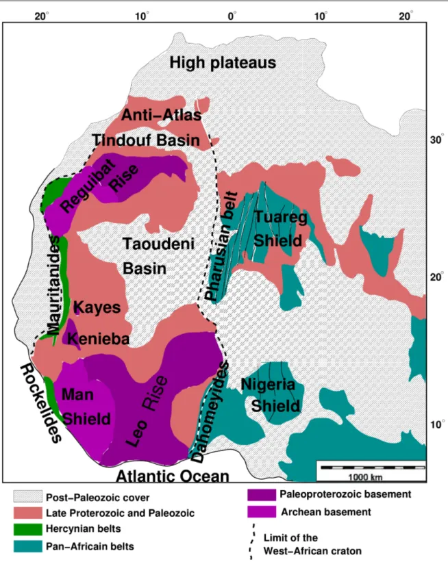
Today, the geology of West Africa is dominated by the West African craton, which is largely covered
58
by the Neoproterozoic to Paleozoic Taoudeni basin (Figure 1). Archean rocks are exposed in the Reguibat
59
shield to the north and the Man-Leo shield to the south. Strong similarities between them suggest that
60
the shields are part of a larger craton that underlies the Basin (Begg et al., 2009). A series of Pan-African
61
and Hercynian belts rings the West African craton: the Pharusian and Dahomeyides belts are regions of
62
nappes along the eastern margin of the craton; the Rokellides and Mauritanides belts run along the western
63
side; and the Anti-Atlas belt is a typical foreland fold-thrust belt, developed by rifting, sedimentation, and
64
volcanism along the northern margin. Such different tectonic environments can give rise to strong lateral
65
and vertical variations in shear wave velocity structure.
66
3 Data and methods
67
For this tomographic study, we used earthquakes and seismicambientnoise data recorded at seismic stations
68
in West Africa and the surrounding regions (Table 1 and Figure 2). We downloaded raw waveform data
69
from the Incorporated Research Institutions for Seismology Data Management Center (IRIS-DMC) and
70
obtained earthquake source parameters from the Global Centroid Moment Tensor catalog (Global CMT).
71
We deconvolved instrument responses from the seismic waveforms before any furtheranalysis.
72
3.1 Earthquake data processing
73
We analyzed vertical component broad-band or long-period seismograms from 342 earthquakes that occurred
74
between 1996 and 2014 recorded at 12 seismic stations. We selected earthquakes with magnitudes M ≥ 5
75
whose epicenters lay between -30◦N, +30◦N, -30◦E and +30◦E, added some M ≥ 4.5 events with clear
76
surface waves, and included some seismic events beyond these coordinates to increase azimuthal coverage.
77
Most of the seismic events in West Africa are shallow (Suleiman et al., 1993), leading to strong fundamental
78
mode Rayleigh waves.
79
Before proceeding with the dispersion analysis, we decimated all the waveforms to 0.25 s (4 Hz), then
80
visualized them and retained those with clear dispersed surface waves. A complete list of earthquake-station
paths retained is available as an Online Resource (Table S1). Example waveforms corresponding to oceanic,
82
ocean-continent, and continental paths are shown in Figure 3.
83
3.2 Ambient noise processing and cross-correlations
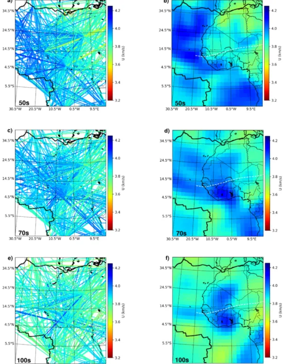
84
We downloaded vertical component data recorded between 1995 and 2015 by 34 broad-band seismic stations
85
and performed cross-correlations between every station-pair to estimate Rayleigh wave Green’s functions.
86
Some stations recorded less than 2 years of data; others suffered interruptions of several months or years.
87
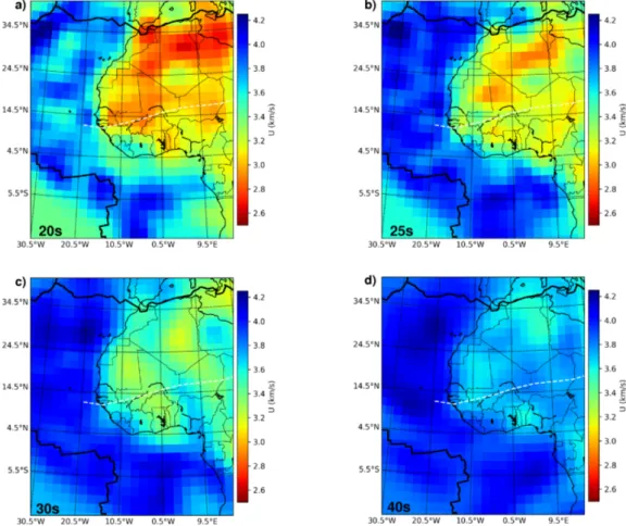
The data availability shown in Figure 4 influenced the number of station pairs available for cross-correlation.
88
Imaging the subsurface structure using seismic noise tomography requires multiple analysis steps to
89
increase the quality of the dispersion curves (Bensen et al., 2007; Lin et al., 2007; Poli et al., 2012). We
90
processed the seismic waveforms station by station, following a procedure similar to that of Zigone et al.
91
(2015) that aims to minimize the negative effects caused by earthquakes, temporally localized incoherent
92
noise sources, and data irregularities. We performed a series of tests before converging on the following
pre-93
processing scheme that maximized the cross-correlation’s signal-to-noise-ratio (defined here as the maximum
94
amplitude divided by the root-mean-square of a noise window from the correlation function’s tail): decimate
95
the signal to 1 s (1 Hz); high-pass filter at 250 s (4 mHz); clip at 15 standard deviations to remove high
96
amplitudes and glitches; cut daily traces into 4-hour time windows; remove strong impulsive signals by
97
discarding windows whose energy exceeds the daily average by over 30%; remove windows with gaps over
98
10% of the total duration; apply spectral domain whitening between 1 and 200 s period (5 and 1000 mHz
99
frequency).
100
After applying this scheme on all our data, we cross-correlated the resulting waveforms across all available
101
station pairs and stacked the correlation functions over the fullest available time period (see for example
102
Bensen et al., 2007). When averaged over a sufficiently long period, the spatial distribution of seismic noise
103
sources tends to homogenize, allowing us to relate the stacked correlation functions for a pair of stations to
104
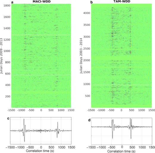
the Green’s function along the path that joins them. Figure 5 shows correlation functions and their resulting
105
stacks for two station pairs, one with 5 years and the other with 12 years of available data. The temporal
106
stability of the correlation functions (Fig. 5a,b) indicates that most of the transient sources were properly
107
removed from the traces by the pre-processing. The signals at positive (causal) and negative (a-causal) lags
108
represent waves travelling in opposite directions between the two stations of a pair. The arrival times of
109
the surface-wave packets are symmetric between the causal and a-causal parts of the stacked correlation
110
functions (Fig. 5c,d) and increase for the more distant station pair. The amplitudes of the causal and
a-111
causal parts are almost identical for the station-pair with 12 years of available data, indicating complete
112
noise homogenization.
113
When ordered with increasing station-pair separation (Fig. 6), the stacked correlation functions filtered
114
between 30-100 s display clear signals that arrive at positive and negative lags with arrival times consistent
with Rayleigh wave group velocities. Such simultaneity combined with only few cases of asymmetric
am-116
plitudes indicates that the overall noise field is close to being diffuse in this period range (near complete
117
homogenization).
118
As in most tomography studies using seismic noise cross-correlation, we symmetrized the correlations by
119
calculating the sum of the causal and a-causal parts for each pair of stations (Shapiro and Campillo, 2004).
120
This process allowed us to take advantage of slight differences in frequency content in the two propagation
121
directions.
122
3.3 Dispersion measurements and path selection
123
We computed the group-velocity dispersion curves for earthquakes and noise cross-correlations using
equiva-124
lent implementations of the same approach: frequency time analysis (Dziewonski et al., 1969; Levshin et al.,
125
1989, 1992; Ritzwoller and Levshin, 1998; Hermann, 2013), which applies a sequence of Gaussian filters at a
126
discrete set of periods and computes the envelope of these filtered signals to create a period group-velocity
127
diagram (see examples in Figures 7 and 8). As the frequency contents of earthquake and noise data differ,
128
we adapted the set of Gaussian filters to each dataset: from 4 to 250 s for earthquakes and from 4 to 120 s
129
for noise correlations.
130
We measured the group-velocity by picking the maximum amplitude of the envelope function at each
131
period and estimated the uncertainty of each measurement as the width of a Gaussian approximation to the
132
envelope function. In order to keep only reliable measurements, we selected the period range on which the
133
maximum of the dispersion diagram corresponded to the fundamental mode Rayleigh wave, while rejecting
134
all parts of the dispersion curves affected by scattered waves, multi-pathing effects, or overlapping overtones.
135
We paid particular attention to the ambient noise dispersion curves, as persistant noise sources, such as the
136
26 s signal identified by Shapiro et al. (2006) in the Gulf of Guinea, can distort them.Figure
137
Figure 7 shows an example of the group-velocity dispersion analysis for the seismogram from Figure 3b,
138
performed using the Hermann (2013) implementation of the multiple filter technique. The Rayleigh wave
139
is well dispersed and produces a simple period group-velocity diagram with a strong, continuous ridge line
140
along which to measure group-velocity. The maximum energy occurs between 30 and 80 s period anddepends
141
on the magnitude of the earthquake (Ms 6.0). Figure 8 shows an equivalent analysis for the symmetrized
142
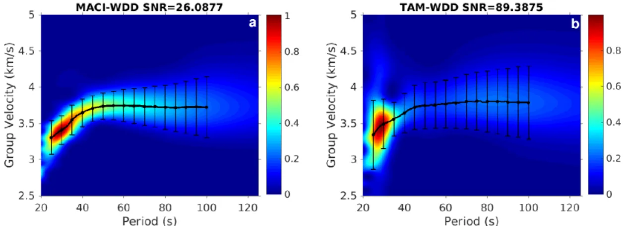
versions of the noise cross-correlation pairs presented on Figure 5, exploiting the Pedersen et al. (2003)
143
implementation of the same multiple filter technique. The maximum energy here occurs between 20 and
144
40 s period and depends on the excitation spectrum of microseismic noise.
145
After measuring the dispersion curves, we used selection criteria specifically designed for each dataset
146
to ensure good quality, coherent measurements.
147
For earthquake data, we followed the approach of Maggi et al. (2006) and Ritzwoller and Levshin (1998)
148
and compared multiple dispersion measurements along repeatedly sampled propagation paths. This allowed
us to identify artefacts such as earthquake source errors and to avoid oversampling of certain paths that
150
could lead to bias in the tomographic models. We formed clusters by grouping all the paths whose starting
151
and ending points occurred within 2◦ of the extremities of a reference path chosen randomly from the
152
data set; we also imposed that no path could belong to more than one cluster. We examined each cluster
153
to identify outlier dispersion curves. After outlier rejection, we selected a representative dispersion curve
154
from each cluster. Not all dispersion curves were part of a cluster;we analysed these single dispersion curves
155
individually for artefacts. We retained 352 fundamental mode Rayleigh wave group-velocity dispersion curves
156
from 147 earthquakes. Table S1 in the Online Resources lists all the corresponding paths with the period
157
ranges retained for the inversion.
158
For cross-correlation data, we excluded dispersion curves computed on cross-correlation functions whose
159
signal-to-noise ratios were smaller than 7. To ensure good sampling of the medium between the two stations,
160
we also excluded group-velocity measurements for which the inter-station distance was smaller than 3
161
wavelengths. We retained 25 stations to estimate inter-station group velocity dispersion curves (Figure 4).
162
Table S2 in Online Resources lists the station pairs with the correspondingperiod ranges retained for the
163
inversion.
164
3.4 Regionalization of group velocity dispersion measurements
165
After the data processing and measurement steps described above, we obtained 4423 individual group
166
velocity measurements between 20 and 100 s period: 3559 from the earthquake data and 864 from the noise
167
cross-correlations.
168
To produce interpretable group velocity maps from these measurements, we solved the standard
tomo-169
graphic problem represented by the linear equation d = G m, where di = xi/Ui is the epicentral distance
170
divided by the group velocity for path i, mj = 1/Uj is the group slowness in cell j of some spatial
dis-171
cretization of the Earth’s surface, and Gij is the length of path i in cell j. We assumed great-circle paths,
172
discretized the problem using a regular latitude/longitude grid, and used the regionalization method
pro-173
posed by Debayle and Sambridge (2004).
174
This computationally efficient method takes into account the measurement uncertainties σd, constrains
175
the lateral smoothness of the inverted model using a horizontal correlation length Lcorr, and controls the
176
amplitude of the perturbations in the inverted model using an a-priori model variance σm. As with all
177
regularization parameters, the criteria for choosing the best combination of Lcorr and σm are somewhat
178
subjective, though they remain based on common sense and make use of a-priori knowledge of the region
179
under study. After testing different discretization grids and values of the regularization parameters, we
180
selected a combination that produced maps consistent with the geological features of the region (sedimentary
181
basins, mobile belt zones, shields, etc.): a 2◦ × 2◦ regular grid and an a-priori model variance σm = 0.05
182
km/s. We selected the Lcorr values for each period through a standard L-curve analysis (Hansen and
O’Leary, 1993), and chose a value near the maximum curvature of the L-curves. This analysis resulted in
184
Lcorr = 300km for periods lower than 30s, Lcorr = 400km between 30s and 70s and Lcorr = 500km for
185
periods longer than 70s.More information on the general effects of increasing or decreasing Lcorr and σm
186
can be found in Maggi et al. (2006), which uses the same inversion method on different data.
187
4 Results
188
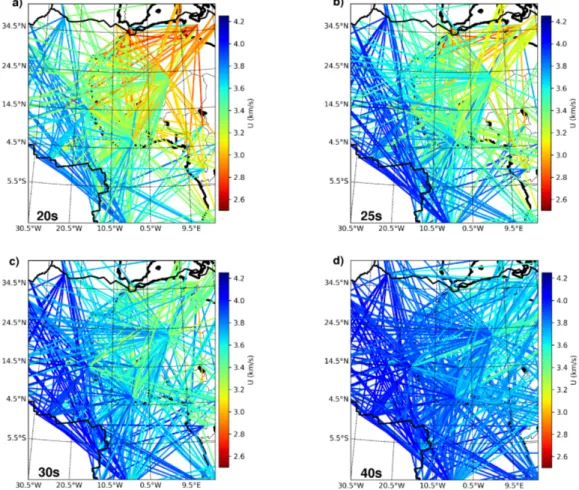
Figure 9 shows the geographical distribution of dispersion measurements from our earthquake and ambient
189
noise joint dataset at periods from 20 to 40 s. These measurements show coherent spatial structure, with slow
190
group velocities for paths contained entirely within the continent, fast group velocities for paths contained
191
entirely within the ocean, and intermediate velocities for paths crossing the ocean-continent boundary.
192
The geographical distribution of measurements for periods between 70 and 100 s shows fewer systematic
193
differences between oceanic and continental paths (Figure 11a,c,e).
194
After applying the Debayle and Sambridge (2004) tomographic inversion method, we obtained the
group-195
velocity maps shown in Figures 10 and 11. The variances of these maps increase at shorter periods, indicating
196
greater heterogeneity at shallow depths. At short periods (Figure 10a-c), we find faster group velocities in
197
the oceanic regions (3.6 to 4 km/s) than in the continental regions (2.8 to 3.2 km/s), due to well-known
198
differences in crustal composition and thickness. These velocities are consistent with crust over 35 km thick
199
in the West African craton and between 9 and 12 km thick in the adjacent ocean, as found by Pasyanos
200
et al. (2004) and Pasyanos and Nyblade (2007). The low group velocities under the Tindouf basin between
201
20 and 40 s period are consistent with its thick sedimentary cover. Those under the Anti-Atlas mountains
202
at 20 and 25 s period are consistent with their recent tectonic history: their Triassic-Jurassic age normal
203
faults reactivated following collision of Africa with Eurasia in the Cenozoic (Gomez et al., 2000). The low
204
velocities under central Algeria between 20 and 40 s period are consistent with the 5 to 6 km thick sediments
205
found in the region by Hadiouche and Jobert (1988).
206
At intermediate periods, despite less pronounced velocity contrasts, we can still distinguish the
Pan-207
African mobile belt zones that form the eastern border of the craton (Figure 11b, also visible in Figure 10b).
208
These zones contain several volcanic fields, have experienced tectono-thermal events within the past 650
209
Ma, and feature higher heat flow and possibly thinner lithosphere than the adjacent West African craton
210
(Lesquer et al., 1989). The Taoudeni basin region shows lower group velocities up to 50 s period, consistent
211
with the thick sedimentary layer found by Begg et al. (2009) (Figures 10 and 11b). We also find slower group
212
velocities in the Paleoproterozoic lithosphere of the Leo Rise compared to those in the adjacent Archean
213
lithosphere of the Man shield at 50 s period (Figure 11b). The low velocity anomalies from 50 to 70 s period
214
in North Africa visible in Figure 11b,d are consistent with the results of Hadiouche and Jobert (1988) who
215
found lower group-velocities extending westward from northeast Africa and attributed them to subduction
216
between the African and European plates.
At long periods (Figure 11d,f), our model displays fast group velocities under the Man-Leo and the
218
Reguibat shields, indicating cold, thick lithospheric roots, and lower group velocities under the mobile belt
219
zone, indicating thinner lithosphere also seen by Priestley et al. (2008). The high velocity root beneath the
220
West African craton extends northward up to the Anti-Atlasin the Priestley et al. (2008) model, while in
221
our model it stops at the southern edge of the Tindouf basin.
222
The roots under the Requibat and Man-Leo shields seem to be separated by a region of lower group
223
velocity that could correspond to the Guinean-Nubian lineament, a major fracture system that extends
224
from the coast of Senegal to the Red Sea (Wilson and Guiraud, 1992; Guiraud et al., 2005). However, the
225
lower group velocities could also be an artefact caused by the thick sediments in the Taoudeni basin (Begg
226
et al., 2009). In order to distinguish between these two interpretations, we would need to consider seismic
227
observables with different vertical sensitivities, for example Rayleigh wave phase velocities, or Love wave
228
phase or group velocities.
229
5 Discussion
230
We produced images of the seismic lithospheric structures of West Africa using group-velocity dispersion
231
curves from both noise correlations and earthquakes. By combining these two sources, we increased the
232
density of surface-wave measurements within this undersampled area and improved the resolution of our
233
seismic models. The resulting Rayleigh-wave group-velocity maps correlate well with major tectonic features
234
in the region. At short periods (Figure 10), our group-velocities highlight differences in crustal thickness:
235
they are fast in the oceans and and slow on the continents. The Tindouf basin and the Anti-Atlas are the
236
slowest continental regions, indicating recent tectonic activity and/or thick sediments. We also observe slow
237
group-velocities under the Taoudeni basin which likely reflects thick sediments (Begg et al., 2009). At an
238
even finer scale, we believe we can see differences between the Paleoproterozoic basement (Leo Rise) and
239
the Archean basement (Man shield), not mentioned in previous studies. At long periods (Figure 11), the
240
fast velocities at the roots of the Man-Leo and the Reguibat shields indicate cold, thick lithosphere under
241
the craton.Our high group velocity anomalies at 100s of period are consistant with estimated lithospheric
242
thickness computed by Pasyanos et al. (2014) and Priestley and Tilmann (2009). Our results are also
243
compatible with the global tomographic model obtained by Ma et al. (2014), which shows high
phase-244
velocity over the West African Croton at low-frequency.Our images show lower group-velocities under the
245
Pan-African mobile belt zones, probably due to thinner lithosphere.
246
When creating tomographic images using ambient noise and earthquakes, we need to ensure that the
247
empirical Green’s functions we obtain from the noise cross-correlations are accurate enough for us to obtain
248
dispersion measurements compatible with those obtained from earthquakes. We tested this in our own
249
dataset by comparing waveforms and dispersion curves from both source types that sample the same region.
250
Figure 12 shows such a comparison for the path between ASCN and TSUM, also sampled by an earthquake
located near ASCN. The surface-waves resemble each other greatly, confirming that the cross-correlations
252
do indeed provide an accurate approximation to the Rayleigh wave Green’s function between the pair of
253
stations (Figure 12b). The two dispersion diagrams also resemble each other between 10 and 50s (Figure
254
12c,d). At longer periods, there seems to be more energy in the cross-correlation than was generated by
255
the moderate magnitude earthquake. Such comparisons convinced us that our earthquake and noise-based
256
surface waves contained similar structural information, and that we could indeed measure and invert them
257
together.
258
Ambient noise and earthquakes provide measurements in complementary period bands. Strong
inter-259
actions between ocean waves and the solid Earth generate most of the microseimic noise recorded by
260
seismological stations and produce stable ambient noise correlation functions in the 1-30s period band
261
(Longuet-Higgings, 1950; Hasselmann, 1963; Campillo and Roux, 2015). At longer periods, the energy of
262
the available noise decreases, which means we need to stack over longer time periods to obtain stable
cross-263
correlation functions (Shapiro and Campillo, 2004; Bensen et al., 2007). Figure 13a shows the number of
264
measurements (paths) as a function of period for both ambient noise and earthquakes. For ambient noise,
265
this number remains constant from 20 s to 40s then decreases rapidly after 50 seconds because we lack noise
266
sources at longer periods. For earthquakes, the number of measurements increases progressively from 20 s
267
to 40s to reach a maximum between 40s to 70s, because the energy provided by earthquakes increases in
268
this period range. Although we obtained surface wave dispersions up to 200s for some large seismic events,
269
these were too few to produce meaningful dispersion maps for periods above 150s, confirming what we
270
have known for two decades now: the reliability of earthquake based Rayleigh-wave group-velocity maps
271
across large continental regions degrades sharplyat periodsbelow 20 s and above 150-200s (Ritzwoller and
272
Levshin, 1998).
273
Our joint dataset provides good spatial coverage from 20 to 100 s period. We obtained many more
group-274
velocity measurements from earthquakes than from seismic noise, however the latter make up one-quarter
275
to one-third of all measurements made below 35s period (see Figure 13a). Noise measurements are the only
276
ones that provide coverage of the eastern part of the region; they also contribute key paths that improve
277
the azimuthal coverage of the more densely sampled regions (see Figure 13b for a comparison of earthquake
278
and noise-based paths at 20 s period). By combining noise and earthquake data, we increased the number
279
of measurements at each period and improved their spatial coverage, both of which are necessary to reduce
280
smearing and biasin group-velocity maps and improve their resolution.
281
The quality of tomography models is controlled by the quantity and quality of the measurements, by
282
the path distribution (density of paths, azimuthal coverage, average path length), and by the weighting and
283
damping applied during inversion (e.g. Vdovin et al., 1999). We used standard checkerboard resolution tests
284
with the same path distribution, measurement uncertainties, correlation length and a-priori model variance
as the real data to investigate the stability and lateral resolution of our group-velocity maps. We created
286
synthetic datasets using checkerboard patterns of different sizes around a mean velocity of 3.7 km/s.
287
Figure 14 shows the synthetic pattern for a10◦× 10◦checkerboard test and the results of three inversions
288
using path distributions and measurement uncertainties observed at 20 s period (note that this is not the
289
period at which we have the densest coverage). Using only earthquake measurements (Figure 14b), we
290
recovered the correct positions of the velocity anomalies in the center and west of the study area. The
291
excessive amplitudes of both positive and negative anomalies in the central region indicate bias caused by
292
paths radiating outwards with almost no crossing paths. Poor azimuthal coverage also caused smearing on
293
the northern and eastern edges of the region. Using only noise measurements (Figure 14c), we recovered more
294
velocity anomalies on the northern and eastern edges, with less bias and smearing thanks to a more balanced
295
azimuthal distribution. By combining the two types of data (Figure 14d), we improved the resolution for
296
the entire study area and reduced the bias in the central region. Eastern Niger and the subduction zone
297
between North Africa and Europe remained poorly resolved due to low path coverage in these areas.
298
Figure 15 shows results of checkerboard tests using the path distribution and measurement uncertainties
299
of the combined dataset at 20 s period and checkerboard sizes of9◦× 9◦ and6◦× 6◦. We recovered correct
300
velocity anomalies over most of the study area for the9◦× 9◦test (Figure 15b), and over the southern part
301
of West Africa for the6◦ × 6◦ test (Figure 15d). We therefore conclude that our combined dataset allows
302
us to achieve an approximate resolution of6 degrein the southern part of West-Africa and9 degreover the
303
rest of the region, with poorer resolution and smearing confined to Eastern Niger and North Africa.
304
Comparing the resolution of different tomographic images can be delicate, as few authors publish
compa-305
rable tests. Of the handful of surface-wave tomography studies that cover West Africa, Pasyanos et al. (2001)
306
could not recover 8◦ × 8◦ checkerboard anomalies in central and West Africa, and Priestley et al. (2008)
307
recovered 10◦ × 10◦ checkerboard anomalies in the same region but showed no results from smaller ones.
308
The resolution of these studies corresponds to the one we obtained using only earthquake data (Figure 14b).
309
We can therefore be confident that adding noise-derived group-velocity measurements to our dataset led to
310
better resolution of West African structures than previous studies.
311
We purposely restricted this study to generating group-velocity maps, without attempting to invert
312
either our original group-velocity dispersion measurements or our group-velocity maps to obtain path-wise
313
or point-wise profiles of VSas a function of depth. Group-velocity depth inversions are notoriously non-linear
314
and unstable, and need to be combined with other information (e.g., group and phase velocities of both
315
Rayleigh and Love waves, fundamental and higher modes) to produde VS(z) profiles usable for structural
316
interpretation.As compiling that additional information may prove difficult with the data available in West
317
Africa, we prefer an alternate strategy. We plan a two-pronged approach: first obtain unbiased
group-318
velocity dispersion maps with full resolution and uncertainty information using the recently developed
319
SOLA Backus-Gilbert inverse methods of Zaroli (2016) and Zaroli et al. (2017), then move away from
dispersion measurements altogether and perform full-waveform inversion of our data-set using 3D
surface-321
wave sensitivity kernels and the SOLA Backus-Gilbert approach to obtain a 3D VS model.
322
6 Conclusion
323
We produced Rayleigh-wave group-velocity maps of west Africa from 20 to 100 s, using data from regional
324
earthquakes and seismic ambient noise cross-correlation. By combining them, we increased the density and
325
azimuthal coverage of our velocity measurements and improved the spatial resolution of our
group-326
velocity maps.
327
At short periods, our Rayleigh-wave group-velocity maps highlight differences in crustal thickness (ocean
328
and continent), recent tectonic activity (e.g. Anti-Atlas), and thick sediments (e.g. Tindouf and Taoudeni
329
basins). At long periods, we found lower velocities due to hot, thin lithosphere under the Pan-African mobile
330
belt and faster velocities due to cold, thick lithosphere under the Man-Leo and Reguibat shields.
331
West Africa can teach us much about the early tectonic history of Earth, if we are willing to listen.
332
Our higher resolution group-velocity maps advance us a step towards answering questions regarding the
333
detailed lithospheric structure and tectonic processes of West Africa; they will also help us generate
im-334
proved models for locating and discriminating small local or regional seismic events. Achieving these goals
335
in full will require adopting new inversion strategies that yield unbiased maps with full resolution and
336
uncertainty information (e.g. SOLA Backus-Gilbert inversions), performing more complete measurements
337
(e.g. surface waveform measurements with their corresponding finite-frequency sensitivity kernels), and,
338
most importantly, acquiring more data by deploying seismic stations in strategic locations.
339
Acknowledgements The research described herein used seismological data from various global networks available through
340
the Incorporated Research Institutions for Seismology (IRIS) Data Management Center (including Africa Array (AF),
341
GEOSCOPE (G), Global Seismograph Network (GSN-IRIS/USGS), Global Telemetered Seismograph Network
(GTSN-342
USAF/USGS), Instituto Superior Tecnico Broadband Seismic Network (IP), IRIS PASSCAL Experiment Stations (XB),
343
MEDNET Project (MN), Morocco-Muenster (3D), and Seismic Network of Tunisia (TT)). We are grateful to the operators
344
of these networks for ensuring the high quality of the data and making them publicly available. Earthquake parameters
345
were obtained from the Global CMT catalog.
346
Y. Ouattara was supported by the Comprehensive Nuclear-Test-Ban Treaty Organization (CTBTO) Young Scientist
347
Award Grant, the Lamto Geophysical Station (Ivory Cost), and the CNRS-INSU TelluS-SYSTER program. Additional
348
support in the form of computer equipment was provided by Institut de Physique du Globe de Strasbourg (IPGS). Y.
349
Ouattara would like to thank Professor A. Diawara, director of the Lamto Geophysical Station, for his advice and moral
350
support in seeking a PhD in seismology in France, and Professor B. C. Sombo for accepting him in his research laboratory
351
in Abidjan and for supervising part of his thesis work.The manuscript benefitted from constructive comments by Michael
352
Pasyanos and Editor Mariano Garcia-Fernandez.
References
354
Becker TW (2012) On recent seismic tomography for the western United States. Geochem Geophys Geosyst
355
13, doi:10.1029/2011GC003977
356
Begg GC, Griffin WL, Natapov LM, O’Reilly SY, Grand SP, O’Neill CJ, Hronsky JMA, Djomani YP,
357
Swain CJ, Deen T, Bowden P (2009) The lithospheric architecture of Africa: Seismic tomography, mantle
358
petrology, and tectonic evolution. Geosphere 5:23–50, doi: 10.1130/GES00179.1
359
Ben-Zion Y (2008) Collective behavior of earthquakes and faults: Continuum-discrete transitions,
360
progressive evolutionary changes, and different dynamic regimes. Reviews of Geophysics 46,
361
doi:0.1029/2008RG000260
362
Bensen GD, Ritzwoller MH, Barmin MP, Levshin AL, Lin F, Moschetti MP, Shapiro NM, Yang Y (2007)
363
Processing seismic ambient noise data to obtain reliable broad-band surface wave dispersion
measure-364
ments. Geophys J Int 169:1239–1260, doi: 10.1111/j.1365-246X.2007.03374.x
365
Bills BG, Adams KD, Wesnousky SG (2007) Cosity structure of the crust and upper mantle in western
366
Nevada from isostatic rebound patterns of the late Pleistocene Lake Lahontan high shoreline. J Geophys
367
Res 112, doi:10.1029/2005JB003941
368
Binks RM, Fairhead JD (1992) A plate tectonic setting for Mesozoic rifts of West and Central Africa.
369
Tectonophysics 213:141–151
370
Bird P (2003) An updated digital model of plate boundaries. Geochem Geophys Geosyst 4,
371
doi:10.1029/2001GC000252
372
Campillo M, Roux P (2015) Crust and Lithospheric Structure - Seismic Imaging and Monitoring with
373
Ambient Noise Correlations. In: Treatise on Geophysics, Elsevier, pp 391–417
374
Chanard K, Avouac J, Ramillien G, Genrich J (2014) Modeling deformation induced by seasonal variations
375
of continental water in the Himalaya region: Sensitivity to Earth elastic structure. Journal of Geophysical
376
Research: Solid Earth 119:5097–5113
377
Craig TJ, Chanard K, Calais E (2017) Hydrologically-driven crustal stresses and seismicity in the New
378
Madrid Seismic Zone. Nature Communications 8:2143, doi:10.1038/s41467-017-01696-w
379
Debayle E, Sambridge M (2004) Inversion of massive surface wave data sets: Model construction and
reso-380
lution assessment. J Geophys Res 109, doi:10.1029/2003JB002652
381
Djomani YHP (1993) Apport de la gravim´etrie `a l ´etude de la lithosph`ere continentale et implications
382
g´eodynamiques : Etude d’un bombement intraplaque : Le massif de l’Adamaoua (Cameroun). Th`ese de
383
Doctorat, Universit´e PARIS Xl ORSAY, Sp´ecialit´e : G´eophysique p 229
384
Dorbath L, Montagner JP (1983) Upper mantle heterogeneities in Africa deduced from Rayleigh wave
385
dispersion. Physics of the Earth and Planetary Interieur 32:218–225
Dziewonski A, Bloch S, Landisman M (1969) A technique for the analysis of transient seismic signals. Bull
387
seis Soc Am 59:427–444
388
Fairhead JD, Reeves CV (1977) Teleseismic delay times, bouguer anomalies and inferred thickness of the
389
african lithosphere. Earth and Planetary Science Letters 36:63–76
390
Gangopadhyay A, Pulliam J, Sen MK (2007) Waveform modelling of teleseismic S, Sp, SsPmP, and
shear-391
coupled PL waves for crust- and upper-mantle velocity structure beneath Africa. Geophys J Int 170:1210–
392
1226, doi: 10.1111/j.1365-246X.2007.03470.x
393
Gomez F, Beauchamp W, Barazangi M (2000) Role of the Atlas Mountains (Northwest Africa) within the
394
African-Eurasian Plate-Boundary Zone. Geology 28(9):775–778, doi: doi.org/10.1130/0091-7613
395
Guiraud R, Bosworth W, Thierry J, Delplanque A (2005) Phanerozoic geological evolution of Northern and
396
Central Africa: An overview. Journal of African Earth Sciences 43:83–143
397
Hadiouche O, Jobert N (1988) Geographical distribution of surface-wave velocities and 3-D upper-mantle
398
structure in Africa. Geophysical Journal 95:87–109
399
Hadiouche O, Jobert N, Montagner JP (1989) Anisotropy of the African continent inferred from surface
400
waves. Phys Earth Planet Inter 58:61–89
401
Hansen PC, O’Leary DP (1993) The use of the L-curve in the regularization of discrete ill-posed problems.
402
SIAM J Sci Comp 14(6):1487–1503
403
Hasselmann K (1963) A Statistical Analysis of the Generation of Microseisms. Reviews of Geophysics and
404
Space Physics 1:177–210
405
Hazler SE, Sheean AF, McNamara DE, Walter WR (2001) One-dimensional Shear Velocity Structure of
406
Northern Africa from Rayleigh Wave Group Velocity Dispersion. Pure appl Geophys 158:1475–1493
407
Hermann RB (2013) Computer programs in seismology: An evolving tool for instruction and research.
408
Seismological Research Letters 84:1081–1088, doi:10.1785/0220110096
409
Lesquer A, Bourmatte A, Ly S, Dautria J (1989) First heat flow determination from the central Sahara
410
:relationship with the Pan-African belt and Hoggar domal uplift. Journal of African Earth Sciences 9:41–
411
48
412
Levshin A, Ratnikova L, Berger J (1992) Peculiarities of surface wave propagation across central Eurasia.
413
Bull seism Soc Am 82:2464–2493
414
Levshin AL, Yanovskaya TB, Lander AV, Bukchin BG, Barmin MP, Ratnikova LI, Its EN (1989) Seismic
415
Surface Waves in a Laterally Inhomogeneous Earth. Kluwer, Dordrecht
416
Lin FC, Ritzwoller MH, Townend J, Bannister S, Savage MK (2007) Ambient noise Rayleigh wave
tomog-417
raphy of New Zealand. Geophys J Int 170:649–666, doi: 10.1111/j.1365-246X.2007.03414.x
418
Longuet-Higgings M (1950) A theory of the origin of microseisms. Philosophical Transactions of the Royal
419
Society of London A243(857):1–35
Ma Z, Masters G, Laske G, Pasyanos M (2014) A comprehensive dispersion model of surface wave phase
421
and group velocity for the globe. Geophys J Int 199:113–135, doi: 10.1093/gji/ggu246
422
Maggi A, Debayle E, Priestley K, Barruol G (2006) Multimode surface waveform tomography of the
423
Pacific Ocean: a closer look at the lithospheric cooling signature. Geophys J Int 166:1384–1397, doi:
424
10.1111/j.1365-246X.2006.03037.x
425
Pasyanos ME, Nyblade AA (2007) A top to bottom lithospheric study of Africa and Arabia. Tectonophysics
426
444:27–44, doi:10.1016/j.tecto.2007.07.008
427
Pasyanos ME, Walter WR, Hazler SE (2001) A Surface Wave Dispersion Study of the Middle East and
428
North Africa for Monitoring the Comprehensive Nuclear-Test-Ban Treaty. Pure and Applied Geophysics
429
158:1445–1474
430
Pasyanos ME, Walter WR, Flanagan MP, Goldstein P, Bhattacharyya J (2004) Building and Testing an a
431
priori Geophysical Model for Western Eurasia and North Africa. Pure Appl Geophys 161:235–181, doi:
432
10.1007/s00024-003-2438-5
433
Pasyanos ME, Masters TG, Laske G, Ma Z (2014) LITHO1.0: An updated crust and lithospheric model of
434
the Earth. Earth, J Geophys Res Solid Earth 119:2153–2173, doi:10.1002/2013JB010626
435
Pedersen HA, Mars J, Amblard PO (2003) Improving group velocity measurements by energy reassignment.
436
Geophysics 68:677–684
437
Poli P, Pedersen HA, Campillo M, the POLENET/LAPNET Working Group (2012) Noise directivity and
438
group velocity tomography in a region with small velocity contrasts: the northern Baltic Shield. Geophys
439
J Int 192:413–424, doi: 10.1093/gji/ggs034
440
Priestley K, Tilmann F (2009) Relationship between the upper mantle high velocity seismic lid and the
441
continental lithosphere. Lithos 109, doi:10.1016/j.lithos.2008.10
442
Priestley K, McKenzie D, Debayle E, Pilidou S (2008) The African upper mantle and its relationship to
443
tectonics and surface geology. Geophys J Int 175:1108–1126, doi: 10.1111/j.1365-246X.2008.03951.x
444
Ritsema J, van Heijst H (2000) New seismic model of the upper mantle beneath Africa. Geology 28:63–66
445
Ritzwoller MH, Levshin AL (1998) Eurasian surface wave tomography : Group velocities. Journal of
Geo-446
physical Research 103:4839–4878
447
Ritzwoller MH, Shapiro NM, Levshin AL, Leahy GM (2001) Crustal and upper mantle structure beneath
448
Antarctica and surrounding oceans. Journal of Geophysical Research 106:30645–30670
449
Romanowicz B (2003) Global Mantle Tomography: Progress Status in the Past 10 Years. Annual Review
450
of Earth and Planetary Sciences 31:303–328, doi:10.1146/annurev.earth.31.091602.113555
451
Sebai A, Stutzmann E, Montagner JP, Sicilia D, Beucler E (2006) Anisotropic structure of the African
452
upper mantle from Rayleigh and Love wave tomography. Physics of the Earth and Planetary Interiors
453
155:48–62, doi:10.1016/j.pepi.2005.09.009
Shapiro NM, Campillo M (2004) Emergence of broadband Rayleigh waves from correlations of the ambient
455
seismic noise. Geophys Res Lett 31, doi:10.1029/2004GL019491
456
Shapiro NM, Campillo M, Stehly L, Ritzwoller MH (2005) High-Resolution Surface-Wave Tomography from
457
Ambient Seismic Noise. Science 307:1615–1618
458
Shapiro NM, Ritzwoller MH, Bensen GD (2006) Source location of the 26 sec microseism from
cross-459
correlations of ambient seismic noise. Geophys Res Lett 33, doi:10.1029/2006GL027010
460
Shen W, Ritzwoller MH (2016) Crustal and uppermost mantle structure beneath the United States. J
461
Geophys Res Solid Earth 121:4306–4342, doi:10.1002/2016JB012887
462
Shen W, Ritzwoller MH, Schulte-Pelkum V (2013) A 3-D model of the crust and uppermost mantle beneath
463
the Central and Western US by joint inversion of receiver functions and surface wave dispersion. Journal
464
of Geophysical Research: Solid Earth 118:262–176, doi:10.1029/2012JB009602
465
Suleiman AS, Doser DI, Yarwood DR (1993) Source parameters of earthquakes along the coastal margin of
466
West Africa and comparisons with earthquakes in other coastal margin settings. Tectonophysics 222:79–91
467
Vdovin O, Rial JA, Levshin AL, Ritzwoller MH (1999) Group-velocity tomography of South America and
468
the surrounding oceans. Geophys J Int 136:324–340
469
Villasenor A, Ritzwoller M, Levshin A, Barmin M, Engdahl E, Spakman W, Trampert J (2001) Shear
470
velocity structure of central Eurasia from inversion of surface wave velocities. Physics of the Earth and
471
Planetary Interiors 123:169–184
472
Wilson M, Guiraud R (1992) Magmatism and rifting in Western and Central Africa, from Late Jurassic to
473
Recent times. Tectonophysics 213:203–225
474
Yang Y, Li A, Ritzwoller MH (2008a) Crustal and uppermost mantle structure in southern Africa
re-475
vealed from ambient noise and teleseismic tomography. Geophys J Int 174:235–248, doi:
10.1111/j.1365-476
246X.2008.03779.x
477
Yang Y, Ritzwoller MH, Lin FC, Moschetti MP, Shapiro NM (2008b) Structure of the crust and uppermost
478
mantle beneath the western United States revealed by ambient noise and earthquake tomography. J
479
Geophys Res 113, doi:10.1029/2008JB005833
480
Yao H, Beghein C, van der Hilst RD (2008) Surface wave array tomography in SE Tibet from ambient
481
seismic noise and two-station analysis – II. Crustal and upper-mantle structure. Geophys J Int 173:205–
482
219, doi:10.1111/j.1365-246X.2007.03696.x
483
Yao H, van der Hilst RD, Montagner J (2010) Heterogeneity and anisotropy of the lithosphere of SE Tibet
484
from surface wave array tomography. J Geophys Res 115, doi:10.1029/2009JB007142
485
Zaroli C (2016) Global seismic tomography using Backus-Gilbert inversion. Geophysical Journal
Interna-486
tional 207, doi:10.1093/gji/ggw315
487
Zaroli C, Koelemeijer P, Lambotte S (2017) Toward Seeing the Earth’s Interior Through Unbiased
Tomo-488
graphic Lenses. Geophysical Research Letters 44, doi:10.1002/2017GL074996
Zigone D, Ben-Zion Y, Campillo M, Roux P (2015) Seismic Tomography of the Southern California Plate
490
Boundary Region from Noise-Based Rayleigh and Love Waves. Pure and Applied Geophysics 172:1007–
491
1032, doi:10.1007/s00024-014-0872-1
Table 1 Seismic stations used in this study. Stations indicated by * were used for dispersion measurements for both earthquake and seismic noise data; stations indicated by ** were used only for earthquakes; the others were used only for ambient noise cross-correlation. Network initials are as follows: Africa Array (AF), GEOSCOPE (G), Global Seismograph Network (GSN-IRIS/USGS), Global Telemetered Seismograph Network (GTSN-USAF/USGS), Instituto Superior Tecnico Broadband Seismic Network (IP), IRIS PASSCAL Experiment Stations (XB), MEDNET Project (MN), Morocco-Muenster (3D), and Seismic Network of Tunisia (TT).
Station Network Latitude(◦N ) Longitude(◦E) Instrument Location ID
ASCN* II -7.9327 -14.3601 Trillium 120 BB 10 BGCA GT 5.1763 18.4242 KS-54000 CM01 XB 2.3890 9.8340 Guralp CMG3T 02 CM10 XB 4.2230 10.6190 Guralp CMG3T 02 CM20 XB 6.2250 10.0540 Guralp CMG3T 02 CM30 XB 9.7570 13.9500 Guralp CMG3T 02 CMLA** II 37.7637 -25.5243 Streckeisen STS-2 10 DBIC* GT 6.6701 -4.8565 KS-54000 00 IFE AF 7.5466 4.4569 EP-105 KOWA* IU 14.4967 -4.0140 Trillium 240 BB 10 MACI IU 28.2502 -16.5081 Streckeisen STS-1V/VBB MBO* G 14.3920 -16.9554 Streckeisen STS-1 10 MM07 3D 30.2584 -5.6084 Trillium 120 s MM13 3D 30.5392 -9.5835 Trillium 120 s MSKU* IU -1.6557 13.6116 Streckeisen STS-1V/BB 00 MTOR IP 28.4948 -9.8487 Streckeisen STS-2/120 s PM01 XB 35.7016 -5.6543 Guralp CMG3T RTC MN 33.9881 -6.8569 Streckeisen STS-1V/VBB SACV* II 14.9702 -23.6085 Trillium 120 BB 10 SEHL* II -15.9588 -5.7457 Streckeisen STS-2 10
SVMA AF 16.8440 -24.9250 Guralp CMG-3ESP/100s
TAM* G 22.7914 5.5283 Streckeisen STS-1 00
TATN* TT 32.5787 10.5292 Streckeisen STS-2/120 s 00
THTN* TT 35.5616 8.6881 Streckeisen STS-2/G3 00
TSUM* IU -19.2022 17.5838 Streckeisen STS-1H/VBB
Fig. 2 Locations of stations used in this study. Squares indicate stations used for dispersion measurements using earthquake data; triangles indicate stations used for cross-correlation analysis.
Fig. 3 Examples of vertical-component velocity seismograms used for dispersion measurements, filtered between 20 s and 100s. Station responses have been removed and amplitudes have been scaled. Station names and epicentral distances are shown. Events parameters from the Global CMT catalog: (a) 15/05/2011, Ms 6.1, depth 12.78 km (0.87◦N, 25.62◦W); (b) 29/11/2011, Ms 6.0, depth 12 km (1.28◦S, 15.60◦W); (c) 19/12/2009, Ms 6.0, depth 12 km (10.02◦S, 33.93◦E).
Fig. 4 Data availability for all stations used for cross-correlation analysis. Good quality stations (in dark blue) yielded cross-correlation functions with signal-to-noise ratios greater than 7. These were used to create group-velocity maps.
Fig. 5 Cross-correlograms (a, b) and stacks (c, d) filtered between 30 and 100 s for two station pairs. Panels (a) and (c) correspond to the station-pair MACI - WDD (3034 km distance) stacked from 2009 to 2013; pannels (b) and (d) correspond to station pair TAM - WDD (1687 km distance) stacked from 2003 to 2014.
Fig. 6 Stacked vertical component cross-correlation functions filtered around 30 and 100 s and ordered with increasing station distance.
Fig. 7 Example of group velocity measurements using the Hermann (2013) implementation of the multiple filter technique on the seismogram from Figure 3b: The left panel shows the spectral amplitude as a function of period, the center panel shows the contours of the period group-velocity diagram that were used to make the dispersion measurement, and the right panel shows the waveform itself. The colors on the period group-velocity diagram indicate relative energy. The measured dispersion curve is indicated by red dots on the spectral amplitude plot and white dots on the period group-velocity diagram.
Fig. 8 Group velocity dispersion diagrams for symmetric component. The thick black curves indicate the measured Rayleigh wave dispersion curves; the error-bars indicate 1-σ uncertainties; the color scale indicates relative energy. The maximum energy is observed at short period.
Fig. 9 Path coverage maps for group-velocity measurements at 20, 25, 30 and 40 s period. The color of each path is given by the corresponding group-velocity measurement.
Fig. 10 Group-velocity maps for 20, 25, 30 and 40 s period, obtained by inverting the measurements shown in Figure 9. The colorscale indicates group-velocity. The white dashed line represents the Guinean-Nubian lineament (Guiraud et al., 2005). Black thick lines show the plate boundaries (Bird, 2003).
Fig. 11 Path coverage (a, c, e) and group-velocity maps (b, d, f) for 50, 70 and 100 s period. The colorscale indicates group-velocity.The white dashed line represents the Guinean-Nubian lineament (Guiraud et al., 2005). Black thick lines show the plate boundaries (Bird, 2003).
Fig. 12 Comparison of seismograms and dispersion curves from the 2000/06/16 Mw 5.0 earthquake (epicenter near ASCN station) recorded by TSUM station and the cross-correlation of seismic ambient noise between the station-pair ASCN-TSUM. The epicentral distance is 3609 km and inter-station distance is 3667 km; we corrected the earthquake waveform for the 58 km difference in distance assuming an average group velocity of 3.63 km/s and filtered the seismograms between 20 and 40 s. (a) Location of earthquake (yellow star) and stations (red triangles). (b) Filtered waveforms from the earthquake (red) and noise correlation (black); the blue rectangle indicates the surface wave packets. (c) and (d) Dispersion diagram of the earthquake and seismic ambient noise cross-correlation respectively.
Fig. 13 (a) Number of group-velocity measurements at each period obtained from earthquakes (blue) and ambient noise correlations (red). (b) Path coverage at 20 s period.
Fig. 14 Checkerboard tests for horizontal resolution with10◦× 10◦horizontal anomalies. (a) Input model. (b), (c), and
(d) Models after inversion using: (b) only earthquake measurements; (c) only noise measurements; (d) both earthquake and noise measurements.
Fig. 15 Checkerboard tests for9◦× 9◦ and6◦ × 6◦using the full path distribution and measurement uncertainties at
20 s. (a) and (c) Synthetic input models for9 degreesand6 degrees. (b) and (d) Output models corresponding to (a) and (c).