HAL Id: hal-00299450
https://hal.archives-ouvertes.fr/hal-00299450
Submitted on 13 Sep 2007
HAL is a multi-disciplinary open access
archive for the deposit and dissemination of
sci-entific research documents, whether they are
pub-lished or not. The documents may come from
teaching and research institutions in France or
abroad, or from public or private research centers.
L’archive ouverte pluridisciplinaire HAL, est
destinée au dépôt et à la diffusion de documents
scientifiques de niveau recherche, publiés ou non,
émanant des établissements d’enseignement et de
recherche français ou étrangers, des laboratoires
publics ou privés.
Pre-earthquake signals ? Part I: Deviatoric stresses turn
rocks into a source of electric currents
F. T. Freund
To cite this version:
F. T. Freund. Pre-earthquake signals ? Part I: Deviatoric stresses turn rocks into a source of
elec-tric currents. Natural Hazards and Earth System Science, Copernicus Publications on behalf of the
European Geosciences Union, 2007, 7 (5), pp.535-541. �hal-00299450�
www.nat-hazards-earth-syst-sci.net/7/535/2007/ © Author(s) 2007. This work is licensed under a Creative Commons License.
Natural Hazards
and Earth
System Sciences
Pre-earthquake signals – Part I: Deviatoric stresses turn rocks into a
source of electric currents
F. T. Freund
NASA Ames Research Center, 242-4, Moffett Field, CA 94035, USA
Carl Sagan Center, SETI Institute, 515 N. Whisman Road, Mountain View, CA 94043, USA Department of Physics, San Jose State University, San Jose, CA 95192-0106, USA
Received: 13 June 2007 – Accepted: 7 August 2007 – Published: 13 September 2007
Abstract. Earthquakes are feared because they often strike
so suddenly. Yet, there are innumerable reports of
pre-earthquake signals. Widespread disagreement exists in the geoscience community how these signals can be generated in the Earth’s crust and whether they are early warning signs, related to the build-up of tectonic stresses before major seis-mic events. Progress in understanding and eventually using these signals has been slow because the underlying physi-cal process or processes are basiphysi-cally not understood. This has changed with the discovery that, when igneous or high-grade metamorphic rocks are subjected to deviatoric stress, dormant electronic charge carriers are activated: electrons and defect electrons. The activation increases the number density of mobile charge carriers in the rocks and, hence, their electric conductivity. The defect electrons are associ-ated with the oxygen anion sublattice and are known as posi-tive holes or pholes for short. The boundary between stressed and unstressed rock acts a potential barrier that lets pholes pass but blocks electrons. Therefore, like electrons and ions in an electrochemical battery, the stress-activated electrons and pholes in the “rock battery” have to flow out in different directions. When the circuit is closed, the battery currents can flow. The discovery of such stress-activated currents in crustal rocks has far-reaching implications for understanding pre-earthquake signals.
1 Introduction
Seismologists use earthquakes as “flash lights” to illuminate the interior of the Earth. Information extracted from the propagation of seismic waves has produced great insights into the hidden structure of our dynamic planet. Unfortu-nately, earthquakes are erratic “flash lights” that seem to go
Correspondence to: F. T. Freund
off at unpredicted times and at unpredicted places. Since they often lead to destruction and death, it is understandable that seismologists have endeavored to find ways to predict – within limits as narrow as possible – time, place and magni-tude of major seismic events (Gokhberg et al., 1995; Lom-nitz, 1994; Milne, 1899, Rikitake, 1976 #452; Sykes et al., 1999; Turcotte, 1991; Wyss and Dmowska, 1997). However, using the “flash lights” is different from understanding when and where a “flash” might go off. The two require different skills and different tools.
Though the seismological models have become ever more sophisticated and tend to take into account ancillary infor-mation (Holliday et al., 2005; Keilis-Borok, 2002; Rundle et al., 2003), the tools of seismology are blunt when it comes to recognizing the build-up of stress before the rupture.
At the same time it has been known for a long time that the Earth sends out a bewildering array of non-seismic
sig-nals before major events (Tributsch, 1984).
Understand-ing how these signals are generated and what information they may provide has remained an elusive goal (Bernard et al., 1997; Hough, 2002; Kagan, 1997; Kanamori, 1996; Knopoff, 1996; Park, 1997; Uyeda, 1998).
1.1 Nature of pre-earthquake signals
The dilatancy theory (Brace et al., 1966) fits a simple me-chanical concept. It is based on the observation that, when rocks are stressed, they expand normal to the stress vector and change their pore volume. This can account for bulging of Earth’s surface and for changes in the resistivity due to pore water (Brace, 1975).
1.2 Earthquake lights
Earthquake lights have been observed since ancient times (Derr, 1973; Galli, 1910; Mack, 1912; Tributsch, 1984). Based on over 1500 reports, Musya (Musya, 1931) stated: “The observations were so abundant and so carefully made
536 F. T. Freund: Pre-earthquake signals – Part I that we can no longer feel much doubt as to the reality of
the phenomena” (Terada, 1931). Nonetheless, doubts per-sisted in the scientific community even beyond 1960s when EQLs were photographed during an earthquake swarm at Matsushiro, Japan (Yasui, 1973). Hedervari and Nosczticz-ius (1985) covered many observations in Europe. St-Laurent (2000) evaluated reports of luminous phenomena sighted at the time of the Saguenay earthquake in Canada. Tsukuda (1997) reported luminous phenomena associated with the 16 January 1995 Kobe earthquake. Similar observations were made in Mexico (Araiza-Quijano and Hern´andez-del-Valle, 1996) and other seismically active regions (King, 1983; Lomnitz, 1994).
1.3 Low frequency electromagnetic emissions
Low frequency electromagnetic (EM) emissions possibly re-lated to pre-earthquake activity have attracted attention over the past 10–20 years (Fujinawa and Takahashi, 1990; Ger-shenzon and Bambakidis, 2001; Gokhberg et al., 1982; Molchanov and Hayakawa, 1998; Nitsan, 1977; Vershinin et al., 1999; Yoshida et al., 1994; Yoshino and Tomizawa,
1989). Other authors report local magnetic field
anoma-lies (Fujinawa and Takahashi, 1990; Gershenzon and Bam-bakidis, 2001; Kopytenko et al., 1993; Ma et al., 2003; Yen et al., 2004; Zlotnicki and Cornet, 1986) or increases in radio-frequency noise (Bianchi and al., 1984; Hayakawa, 1989; Martelli and Smith, 1989). Mercer and Klemperer (Merzer and Klemperer, 1997) modeled the EM emissions prior to the 1989 M=7.1 Loma Prieta earthquake (Fraser-Smith et al., 1990) assuming streaming potentials caused by the move-ment of water along the fault plane. Sometimes no EM emis-sions are recorded, which has caused considerable conster-nation in the science community (Karakelian et al., 2002).
1.4 Ionospheric perturbation
The ionosphere marks the transition from the Earth’s atmo-sphere to the vacuum of space. It is a highly dynamic re-gion where the solar radiation creates a plasma of ions and free electrons, which partly decays during the night. Pro-longed ionospheric perturbations were observed before the great 1960 Chilean earthquake (Warwick et al., 1982) and the 1964 “Good Friday” earthquake in Alaska (Davis and Baker, 1965). Changes of the Total Electron Content, TEC, observed days before major events suggest the presence of a positive charge on the Earth’s surface to which the iono-sphere responds (Liperovsky et al., 2000; Liu et al., 2001; Liu et al., 2000; Naaman et al., 2001). A discussion of the pre-earthquake effects is found in Pulinets and Boyarchuk (2004) who favor release of radon at the Earth’s surface as the cause of the reported ionospheric perturbations.
1.5 “Thermal Anomalies”
Non-stationary areas of enhanced infrared (IR) emission, linked to impending (Gornyi et al., 1988; Qiang et al., 1991; Qiang et al., 1990; Srivastav et al., 1997) with apparent land
surface temperature variations on the order of 2–4◦C. The
ef-fect has become known as “thermal anomalies”. The cause has remained enigmatic (Ouzounov et al., 2007; Srivastav et al., 1997; Tramutoli et al., 2005; Tronin, 2002; Tronin et al., 2004). The rapidity of the temperature variations rules out a flow of Joule heat from deep below. Several alternative processes have been invoked: Rising well water levels and changing moisture contents in the soil; near-ground air ion-ization due to radon emission leading to the condensation of water vapor and the release of latent heat; emanation of warm
gases (Gornyi et al., 1988), in particular of CO2(Quing et al.,
1991; Tronin, 1999; Tronin, 2002).
1.6 Other pre-earthquake signals
There are claims of other pre-earthquake phenomena such as differences in ground potentials (Varotsos et al., 1993, 1986; Varotsos, 2005), low-lying fog and unusual clouds (Tsukuda, 1997), and of course the rich folklore of abnormal animal behavior (Tributsch, 1984).
1.7 Common traits among non-seismic pre-earthquake
sig-nals
Many pre-earthquake signals require transient electric
cur-rents in the Earth’s crust. Electric currents arising from
streaming potentials are well known (Bernab´e, 1998; Jou-niaux et al., 2000; Merzer and Klemperer, 1997; Morrison et al., 1989). Currents due to piezoelectric voltages generated in quartz-bearing rocks have been invoked to explain pre-earthquake low-frequency EM emissions (Gershenzon and Bambakidis, 2001; Ogawa and Utada, 2000; Sasai, 1991). However, no consensus of opinion has emerged.
2 Experimental
Important properties of rocks have been profoundly misun-derstood or misinterpreted in the past, specifically the electri-cal properties of igneous and high-grade metamorphic rocks, which make up the bulk of Earth’s crust in the depth range where most earthquakes occur, about 7–35 km.
At the root lies the fact that, in the geosciences, electri-cal conductivity of rocks is typielectri-cally, often exclusively dis-cussed in terms of ionic conductivity (high temperatures, par-tial melts) or electrolytical conductivity (low temperatures, fluids). However, from a solid state physics viewpoint there may be other mechanisms that can contribute significantly. One of these mechanisms arises from the fact that not all oxygen anions exist in their common 2- valence state but in
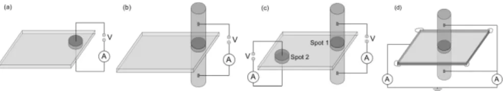
Figure 1. Different ways to measure electrical conductivity. (a): Standard procedure, no load; (b): under
Fig. 1. Different ways to measure electrical conductivity. (a): Standard procedure, no load; (b): under load; (c): measuring at two places, one under load; (d): measuring a battery current.
the 1- valence state. Though valence fluctuations on the oxy-gen anion sublattice may appear to be of interest only to the narrowest of the specialists, they can have far-reaching con-sequences the capability of rocks to generate electric currents and, hence, to generate electric or electromagnetic signals.
To provide some background I start with a tutorial about electrical conductivity measurements. The electrical conduc-tivity is typically measured with a set-up such as depicted in Fig. 1a: a voltage is applied between a pair of electrodes on opposite surfaces of a flat sample and the current is recorded with an ammeter. If the effect of stress is to be studied, two pistons may be used to apply a force as shown in Fig. 1b. Figure 1c depicts a set-up, where the conductivity is mea-sured at two places, spot 1 between the pistons and spot 2 where no stress is applied. Conventional wisdom suggests such an experiment will lead to nothing new: the conductiv-ity across spot 2 should not change when stress is applied to spot 1. Figure 1d shows yet another set-up: a circuit with-out a voltage source but a pair of steel pistons at the center, in electrical contact with the rock and connected to ground through one ammeter plus a Cu stripe as a contact along the periphery, connected to ground through a second ammeter. This circuit does not apply a voltage across the rock sample and, hence, will not measure electrical conductivity. Instead it will measure currents that flow out of the stressed rock un-der a self-generated voltage differential between the pistons and the periphery of the rock.
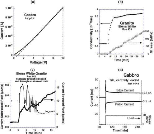
Figure 2a shows a typical current-voltage (I-V) plot recorded with a set-up as in Fig. 1a. The sample is a dry gabbro. Except for the low voltage region, the I-V plot is lin-ear as it should be for an Ohmic response. Figure 2b gives an example for the conductivity of dry granite measured with a set-up as shown in Fig. 1b. During the first 7 min, the current is recorded without applying stress to the rock. The
conduc-tivity before loading is 0.7×10⁻⁶S/m. Upon loading, the
conductivity rises sharply, increasing by a factor of 3–4 to
about 2.5×10⁻⁶Sm and then continues to increase slowly.
Stress-induced increase in the conductivity is commonly ex-plained by better point-to-point contacts between grains un-der load (Glover and Vine, 1992). However, the next experi-ment will show that we are dealing with a more complex and much more interesting phenomenon.
The data shown in Fig. 2c were obtained with a set-up as depicted in Fig. 1c. We measured simultaneously the
cur-rents at spot 1 and at spot 2, i.e. between a pair of electrodes away from the stressed rock volume. The bold line shows the current at spot 1, the thin line the current at spot 2. Af-ter about 6 min, when we began applying the load, the current flowing through the stressed rock increased very rapidly, sim-ilar to what we had observed during the experiment shown in Fig. 2b. In addition, the current flowing through the rock in the unstressed portion also increased significantly. Even when we widened the distance between spot 1 and 2, the ef-fect remained, indicating that spot 1 and spot 2 were “talking to each other electrically” beyond the range over which the mechanical stress was transmitted.
To find out more about this “cross talk” we used the circuit in Fig. 1d where we simply run a wire from the pistons at the center to the Cu contact along the edges. Initially no current flows. When a load is applied to the center, both ammeters in the cirucit record a current as shown in Fig. 2d. The first ammeter records electrons flowing from the pistons to ground. The second ammeter records electrons flowing from ground into the rock. The two currents are of the same magnitude, suggesting that they are in fact the same current. What we have here is, in fact, a battery with electrons flow-ing out from the stressed rock volume through the pistons into the external circuit and reentering the unstressed rock along the edges. A current through the external circuit im-plies a current of the same magnitude through the rock.
2.1 Dormant electronic charge carriers
What Fig. 2d demonstrates is a mechanism, previously un-known, to generate electrical currents in a rock subjected to deviatoric stress (Freund, 2002, 2003). The mechanism is fundamentally different from piezoelectricity. It is based on the fact that a small but non-zero number of the oxygen an-ions in the minerals that make up these rocks are not in their
usual 2- valence state (O2−)but have converted to the 1- state
(O−).
From a semiconductor perspective an O− in a matrix of
O2−represents a defect electron or hole, also known as
pos-itive hole or phole for short. The O− normally form
posi-tive hole pairs, PHP, chemically equivalent to peroxy links,
O3Si-OO-SiO3. In the form of PHPs the O−are electrically
inactive or “dormant”. During deformation, dislocations are generated in large numbers. When they intersect a PHP, the
538 F. T. Freund: Pre-earthquake signals – Part I
external circuit implies that a current of the same magnitude must flow through the rock.
(a) (b)
(c) (d)
Figure 2. Exemplary results obtained with dry rocks using the 4 different circuits depicted in Figure 1
Fig. 2. Exemplary results obtained with dry rocks using the 4 different circuits depicted in Figs. 1a–d. (a): Current-voltage plot indicating essentially a classical ohmic behavior; (b): Significant increase in the electrical conductivity when stress is applied and strongly non-linear current response; (c): bold line: conductivity changes during application of stress through the stressed rock volume; thin line: instant change in the electrical conductivity of the unstressed rock; (d): demonstration of the stressed rock volume turning into a battery (see text).
Figure 3. Experimental set-up with a slab of granite, one end in a press, Cu contacts attached to front and
Fig. 3. Experimental set-up with a slab of granite, one end in a press, Cu contacts attached to front and the back (left); electric circuit with ammeters to measure currents, one between each Cu contact and ground, capacitive sensor to measure the surface charge (upper right); circuit showing the flow of electrons through the outer circuit and the flow of holes through the rock (lower right).
peroxy bond breaks, “waking up” a phole. The phole then becomes a highly mobile electronic charge carrier.
When we stress a portion of a block of igneous rock, a
grayish-white Sierra Nevada granite, 10×15×120 cm3,
insu-late it from the press and ground, as shown in Fig. 3 (left), the stressed portion turns into a battery (Freund et al., 2006). Figure 3 (right, top) shows the electric circuit similar to the one in Fig. 1d. Figure 3 (right, bottom) shows the current flow: electrons, e’, leave the stressed rock, the “source” S, and reenter the rock at the unstressed end. To close the cir-cuit a current of equal magnitude must flow through the rock. This current is carried by pholes. Some are trapped at the rock surface generating a positive surface charge relative to ground. This surface charge is recorded by means of a ca-pacitive sensor visible in the photograph in Fig. 3 (left) as a flat metal plate 0.8 mm above the rock surface.
The stressed rock volume becomes the “source” in which electrons and pholes are co-activated (Freund et al., 2006). There are two points ot be stressed: (i) inside the stressed rock volume the number of charge carriers that is available to transport electric current has gone up, allowing the rock to transport more current than before, in the unstressed state; (ii) There are two kinds of charge carriers, both electronic but one kind (the electrons) representing a negative charge and the other kind (the pholes) representing a positive charge. For both the number density inside the stressed rock volume is higher than outside the stress field. Both would “like” to spread out of the stressed rock volume, if they can.
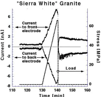
. As one end of the granite slab is load
Fig. 4. As one end of the granite slab is loaded (dotted line) elec-trons flow out of the stressed rock volume to ground (lower curve) and from ground into the unstressed rock (upper curve). The two currents are legs of one and the same circuit.
We conjecture that the boundary between stressed and un-stressed rock acts like a Schottky barrier: it lets holes pass but rejects electrons. This barrier function is illustrated in Fig. 3 (lower right) by the symbol of a diode. Indeed, as shown in Fig. 4, a current carried by positive charge begins to flow as soon as a load is applied. A positive charge layer builds up on the rock surface (not shown), due to trapping of pholes.
In the case of the granite slab, a linear system, the cur-rents increased approximately linearly with applied stress. In Fig. 5, for a planar geometry, the currents increase in a non-linear fashion, very steep at first with strong fluctuations, and then saturate before the modest stress level of 48 MPa is reached. The cause of these fluctuations is unknown. They may be due to coupling, mediated by an internal electric field, between the electron and phole currents flowing out of the stressed rock volume in opposite directions.
Another interesting feature in Fig. 5 is that, when stress is removed slowly, the currents return to zero. The process is repeatable. We have applied the same load-hold-unload-hold program 22 times over a period of 12 h and observed that the currents always return to the same level.
2.2 Rocks turn into batteries
The most important conclusion to be draw from this series of experiments is that, when rocks such as granite or gabbro are subjected to deviatoric stress, they behave as if they were batteries. When stresses are applied, electronic charge carri-ers are activated, both electrons and pholes. In other words, the application of stress charges the battery. Removing the
Fig. 5. Outflow currents from a gabbro tile, 30×30×1 cm3, loaded at the center (∼10 cm3) from 0 to 48 MPa and kept at constant load for 30 min. Currents increase rapidly at beginning, reach a steady state value and decay slowly. Upon unloading currents return to zero.
stress causes the battery to return to an inactive state, ready to be charged again. So far we have not reached a limit of how often we can repeat the process. So long as the stress is well below the threshold of macroscopic damage, in our case about 1/4th the failure strength of the unconstrained rock, the process is repeatable many times.
How much current can be delivered per unit rock volume? In the case of gabbro the rock volume between the pistons in
about 10 cm3. We measure typically 300 pA. If the rock
vol-ume were 1 km3, the outflow current would be on the order
of 30 000 A. By stressing the rock tiles faster, the steady-state outflow currents were found to increase to 50 000 A, plus an
initial spike that can rise to 100 000 A/km3.
In an electrochemical battery the current flowing through the outer circuit is carried by electrons, while the current through the electrolyte is carried by cations. In the case of the rocks, the current flowing through the outer circuit is car-ried by electrons, while the current running through the rock, the internal current, is carried by defect electrons or holes, also known as “positive holes” or pholes for short at briefly outlined above.
Acknowledgements. This work has been supported in part by the
NASA Ames Research Center Director’s Discretionary Fund and by a GEST Fellowship from the NASA Goddard Space Flight Center, Planetary Geodynamics Laboratory. I thank my students and my coworkers A. Takeuchi (supported by a JSPS fellowship) and Dr. Bobby WS Lau (supported through a grant from NGA). Edited by: M. Contadakis
540 F. T. Freund: Pre-earthquake signals – Part I
References
Araiza-Quijano, M. R. and Hern´andez-del-Valle, G.: Some obser-vations of atmospheric luminosity as a possible earthquake pre-cursor, Geofisica Internacional, 35, 403–408, 1996.
Bernab´e, Y.: Streaming potential in heterogenous networks, J. Geo-phys. Res., 103, 20 827–20 841, 1998.
Bernard, P., Pinettes, P., Hatzidimitriou, P. M., et al.: From precur-sors to prediction: a few recent cases from Greece, Geophys. J. Internatl., 131, 467–477, 1997.
Brace, W. F.: Dilatancy-related electrical resistivity change in rocks, Pure Appl. Geophys., 113, 207–217, 1975.
Brace, W. F., Paulding, B. W., and Scholz, C.: Dilatancy in the fracture of crystalline rocks, J. Geophys. Res., 71, 3939–3953, 1966.
Davis, K. and D. M. Baker: Ionospheric effects observed around the time of the Alaskan earthquake of March 28.1964, J. Geophys. Res., 70, 2251–2253, 1965.
Derr, J. S.: Earthquake lights: a review of observations and present theories, Bull. Seismol. Soc. Am., 63, 2177–2187, 1973. Fraser-Smith, A. C., Bernardi, A., McGill, P. R., et al.:
Low-frequency magnetic field measurements near the epicenter of the Ms=7.1 Loma Prieta earthquake, Geophys. Res. Lett., 17, 1465-1468, 1990.
Freund, F.: Charge generation and propagation in rocks, J. Geody-namics, 33, 545–572, 2002.
Freund, F. T.: On the electrical conductivity structure of the stable continental crust, J. Geodynamics, 35, 353–388, 2003.
Freund, F. T., Takeuchi, A., and Lau, B. W.: Electric currents streaming out of stressed igneous rocks - A step towards un-derstanding pre-earthquake low frequency EM emissions, Phys. Chem. Earth, 31, 389–396, 2006.
Fujinawa, Y. and Takahashi, K.: Emission of electromagnetic ra-diation preceding the Ito seismic swarm of 1989, Nature, 347, 376–378, 1990.
Galli, I.: Raccolta e classifzione di fenomeni luminosi osservati nei terremoti, Bolletino della Societa Sismological Italiana, 14, 221– 448, 1910.
Gershenzon, N. and Bambakidis, G.: Modeling of seismo-electromagnetic phenomena, Russian J. Earth Scie., 3, 247–275, 2001.
Glover, P. W. J. and Vine, F. J.: Electrical conductivity of carbon-bearing granulite at raised temperatures and pressures, Nature, 360, 723–726, 1992.
Gokhberg, M. B., Morgounov, V. A., and Pokhotelov, O. A. : Earth-quake Prediction, Gordon and Breach, 1995.
Gokhberg, M. B., Morgounov, V. A., Yoshino, T., and Tomizawa, I.: Experimental measurements of electromagnetic emissions possi-ble related to earthquakes in Japan, J. Geophys. Res., 87, 7824– 7828, 1982.
Gornyi, V. I., Salman, A. G., Tronin, A. A., and Shilin, B. B.: The Earth’s outgoing IR radiation as an indicator of seismic activity, Proc. Acad. Sci. USSR, 301, 67–69, 1988.
Hayakawa, M.: Satellite observation of low latitude VLF radio noise and their association with thunderstorms, J. Geomagn. Geoelectr., 41, 573–595, 1989.
Hedervari, P., & Z. Noszticzius (1985), Recent results concerning earthquake lights, Annales Geophysicae, 3, 705-708.
Hollerman, W. A., Malespin, C., Bergeron, N. P., et al.: Elec-tric currents in granite and gabbro generated by impacts up to
1 km/sec, paper presented at AGU Fall Meeting, AGU, San Fran-cisco, 2006.
Holliday, J. R., Nanjo, K. Z., Tiampo, K. F., et al.: Earthquake fore-casting and its verification, Nonlinear Processes in Geophysics, 12, 965–977, 2005.
Hough, S. E.: Earthshaking Science: What We Know (and Don’t Know) about Earthquakes, 272 pp., Princeton University Press, Princeton, NJ, 2002.
Jouniaux, L., Bernard, M. L., Zamora, M., and Pozzi, J. P.: Stream-ing potential in volcanic rocks from Mount Pel´ee, J. Geophys. Res., 105, 8391–8401, 2000.
Kagan, Y. Y.: Are earthquakes predictable? Geophys, J. Internatl., 131, 505–525, 1997.
Kanamori, H.: A seismologist’s view of VAN, in Earthquake Pre-diction from Seismic Electric Signals, edited by J. Sir Lighthill, pp. 339–345, World Science Publ., Singapore, 1996.
Karakelian, D., Beroza, G. C., Klemperer, S. L., and Fraser-Smith, A. C.: Analysis of ultralow-frequency electrommagnetic field measurements associated with the 1999 M 7.1 Hector Mine, Cal-ifornia, earthquake sequence, Bull. Seismol. Soc. Am., 92, 1513– 2524, 2002.
Keilis-Borok, V.: Earthquake Prediction: State-of-the-Art and Emerging Possibilities, Ann. Rev. Earth Planet. Sci., 30, 1–33, 2002.
King, C.-Y.: Electromagnetic emission before earthquakes, Nature, 301, 377, 1983.
Knopoff, L.: Earthquake prediction: The scientific challenge, Proc. Natl. Acad. Sci. USA, 93, 3719–3720, 1996.
Kopytenko, Y. A., Matiashvili, T., Voronov, P. M., et al.: Detection of ultralow frequency emissions connected with the Spitak earth-quake and its aftershock activity, based on geomagnetic pulsation data at Susheti and Vardzia observatories, Phys. Earth Planet. In-ter., 77, 85–95, 1993.
Liperovsky, V. A., Pokhotelov, O. A., Liperovskaya, E. E., et al.: Modification of sporadic E-layers caused by seismic activity, Surveys in Geophysics, 21, 449–486, 2000.
Liu, J. Y., Chen, Y. I., Chuo, Y. J., and Tsai, H. F.: Variations of ionospheric total electron content during the Chi-Chi earthquake, Geophy. Res. Lett., 28, 1383–1386, 2001.
Liu, J. Y., Chen, Y. I., Pulinets, S. A., et al.: Seismo-ionospheric signatures prior to M=6.0 Taiwan earthquakes, Geophys. Res. Lett., 27, 3113–3116, 2000.
Lomnitz, C.: Fundamentals of Earthquake Prediction, 326 pp., New York, NY, 1994.
Ma, Q.-Z., Jing-Yuan, Y., and Gu, X.-Z.: The electromagnetic anomalies observed at Chongming station and the Taiwan strong earthquake (M=7.5, March 31, 2002), Earthquake, 23, 49–56, 2003.
Mack, K.: Das s¨uddeutsche Erdbeben vom 16. November 1911, Abschnitt VII: Lichterscheinungen, in W¨urtembergische Jahrb¨ucher f¨ur Statistik and Landeskunde, edited, p. 131, Stuttgart, 1912.
Martelli, G. and Smith, P. N.: Light, radiofrequency emission and ionization effects associated with rock fracture, Geophys, J. In-ternatl., 98, 397–401, 1989.
Merzer, M. and Klemperer, S. L.: Modeling low-frequency magnetic-field precursors to the Loma Prieta earthquake with a precursory increase in fault–zone conductivity, Pure Appl. Geo-phys., 150, 217–248, 1997.
Milne, J.: Earthquakes and other Earth Movements, 376 pp., D. Appleton Co., New York, NY, 1899.
Molchanov, O. A. and Hayakawa, M.: On the generation mecha-nism of ULF seimogenic electromagnetic emissions, Phys. Earth Planet. Int., 105, 201-220, 1998.
Morrison, F. D., Williams, E. R., and Madden, T. D.: Streaming po-tentials of Westerly granite with applications, J. Geophys. Res., 94, 12 449–12 461, 1989.
Musya, K.: On the luminous phenomena that attended the Idu earth-quake, November 6th, 1930, Bull. Earthquake Res. Inst., 9, 214– 215, 1931.
Naaman, S., Alperovich, L. S., Wdowinski, S., et al.: Comparison of simultaneous variations of the ionospheric total electron con-tent and geomagnetic field associated with strong earthquakes, Natural Hazards Earth System Sci., 1, 53–59, 2001.
Nitsan, U.: Electromagnetic emission accompanying fracture of quartz-bearing rocks, Geophys. Res. Lett., 4, 333–336, 1977. Ogawa, T. and Utada, H.: Electromagnetic signals related to
inci-dence of a teleseismic body wave into a subsurface piezoelectric body, Earth Planets Space, 52, 253–256, 2000.
Ouzounov, D., Liu, D., Kang, C., et al.: Outgoing Long Wave Ra-diation Variability from IR Satellite Data Prior to Major Earth-quakes, Tectonophysics, 431, 211–220, 2007.
Park, S. K.: Electromagnetic precursors to earthquakes: a search for predictors, Sci. Progr., 80, 65–82, 1997.
Pulinets, S. and Boyarchuk, K.: Ionospheric Precursors of Earth-quakes, 350 pp., Springer Verlag, 2004.
Qiang, Z.-J., Xu, X.-D., and Dian, C.-D.: Abnormal infrared ther-mal of satellite-forewarning of earthquakes, Chinese Sci. Bull., 35, 1324–1327, 1990.
Qiang, Z.-J., Xu, X.-D., and Dian, C.-D.: Thermal infrared anomaly – precursor of impending earthquakes, Chinese Sci. Bull., 36, 319-323, 1991.
Quing, Z., Xiu-Deng, X., and Chang-Gong, D.: Thermal infrared anomaly- precursor of impending earthquakes, Chinese Science Bulletin, 36, 319–323, 1991.
Rundle, J. B., Turcotte, D. L., Shcherbakov, R., et al.: Statistical physics approach to understanding the multiscale dynamics of earthquake fault systems, Rev. Geophys., 1019–1049, 2003. Sasai, Y.: Tectonomagnetic modeling on the basis of the linear
piezomagnetic effect, Bull. Earthq. Res. Inst., Univ. Tokyo, 66, 585–722, 1991.
Srivastav, S. K., Dangwal, M., Bhattachary, A., and Reddy, P. R.: Satellite data reveals pre-earthquake thermal anomalies in Killari area, Maharashtra, Current Science, 72, 880–884, 1997. St-Laurent, F.: The Saguenay, Qu´ebec, earthquake lights of
Novem-ber 1988-January 1989, Seismolog. Res. Lett., 71, 160–174, 2000.
Sykes, L., Shaw, B., and Scholz, C.: Rethinking Earthquake Predic-tion, Pure Appl. Geophys., 155, 207-232, 1999.
Terada, T.: On luminous phenomena accompanying earthquakes, Bull. Earthquake Res. Inst. Tokyo Univ., 9, 225–255, 1931. Tramutoli, V. et al. (2005), Assessing the potential of thermal
in-frared satellite surveys for monitoring seismically active areas: The case of Kocaeli (Izmit) earthquake, August 17, 1999, Re-mote Sens. Environ., 96, 409-426.
Tributsch, H.: When the Snakes Awake: Animals and Earthquake Prediction, 264 pp., MIT Press, Cambridge, Mass, 1984.
Tronin, A. A. (Ed.): Satellite thermal survey application for earth-quake prediction, 717–746 pp., Terra Sci. Publ., Tokyo, Japan, 1999.
Tronin, A. A.: Atmosphere-lithosphere coupling: Thermal anoma-lies on the Earth surface in seismic process, in Seismo-Electromagnetics: Lithosphere-Atmosphere-Ionosphere Cou-pling, edited by: Hayakawa, M. and Molchanov, O. A., pp. 173– 176, Terra Scientific Publ., Tokyo, 2002.
Tronin, A. A., Molchanov, O. A., and Biagi, P. F.: Thermal anoma-lies and well observations in Kamchatka, International Journal of Remote Sensing, 25, 2649–2655, 2004.
Tsukuda, T.: Sizes and some features of luminous sources associ-ated with the 1995 Hyogo-ken Nanbu earthquake, J. Phys. Earth, 45, 73–82, 1997.
Turcotte, D. L. : Earthquake prediction, Annu. Rev. Earth Planet. Sci., 19, 263–281, 1991.
Uyeda, S.: VAN method of short-term earthquake prediction shows promise, EOS Trans. AGU, 79, 573–580, 1998.
Varotsos, P., Alexopoulos, K., Lazaridou, M., and Nagao, T.: Earth-quake predictions issued n Greece by seismic electric signals since February 6, 1990, Tectonophys., 224, 269–288, 1993. Varotsos, P., Alexopoulos, K., Nomicos, K., and Lazaridou, M.:
Earthquake prediction and electric signals, Nature, 322, 120, 1986.
Varotsos, P. A.: The Physics of Seismic Electric Signals (Terra Sci-entific Publ. Co., Tokyo), pp. 388, 2005.
Vershinin, E. F., Buzevich, A. V., Yumoto, K., et al.: Correlation of seismic activity with electromagnetic emissions and variations in Kamchatka region, in Atmospheric and Ionospheric Electro-magnetic Phenomena Associated with Earthquakes, edited by: Hayakawa, M., pp. 513–517, Terra Sci. Publ., Tokyo, Japan, 1999.
Warwick, J. W., Stoker, C., and Meyer, T. R.: Radio emission associated with rock fracture: Possible application to the great Chilean earthquake of May 22, 1960, J. Geophys. Res., 87, 2851–2859, 1982.
Wyss, M. and Dmowska, R. (Eds.): Earthquake Prediction – State of the Art, 272 pp., Birkh¨auser Verlag, 1997.
Yasui, Y.: A summary of studies on luminous phenomena accompa-nied with earthquakes, Memoirs Kakioka Magnetic Observatory, 15, 127–138, 1973.
Yen, H.-Y., Cheng, C-H., Yeh, Y-H., et al.: Geomagnetic fluctua-tions during the 1999 Chi-Chi earthquake in Taiwan, Earth Plan-ets Space, 56, 39-45, 2004.
Yoshida, S., Manjgaladze, P., Zilpimiani, D., et al.: Electromagnetic emissions associated with frictional sliding of rock, in: Electro-magnetic Phenomena Related to Earthquake Prediction, edited by: Hayakawa, M. and Fujinawa, Y., pp. 307-322, Terra Scien-tific, Tokyo, 1994.
Yoshino, T. and Tomizawa, I.: Observation of low-frequency elec-tromagnetic emissions as precursors to the volcanic eruption at Mt. Mihara during November, 1986, Phys. Earth Planet. Inter., 57, 32–39, 1989.
Zlotnicki, J. and Cornet, F. H.: A numerical model of earthquake-induced piezomagnetic anomalies, J. Geophys. Res., B91, 709– 718, 1986.