Global modelling study (GSM TIP) of the ionospheric effects of excited <i>N₂</i>, convection and heat fluxes by comparison with EISCAT and satellite data for 31 July 1990

HAL Id: hal-00316260

https://hal.archives-ouvertes.fr/hal-00316260

Submitted on 1 Jan 1996

HAL is a multi-disciplinary open access

archive for the deposit and dissemination of sci-entific research documents, whether they are pub-lished or not. The documents may come from teaching and research institutions in France or abroad, or from public or private research centers.

L’archive ouverte pluridisciplinaire HAL, est destinée au dépôt et à la diffusion de documents scientifiques de niveau recherche, publiés ou non, émanant des établissements d’enseignement et de recherche français ou étrangers, des laboratoires publics ou privés.

Global modelling study (GSM TIP) of the ionospheric

effects of excited N2, convection and heat fluxes by

comparison with EISCAT and satellite data for 31 July

1990

Yu. N. Korenkov, V. V. Klimenko, M. Förster, V. A. Surotkin, J. Smilauer

To cite this version:

Yu. N. Korenkov, V. V. Klimenko, M. Förster, V. A. Surotkin, J. Smilauer. Global modelling study (GSM TIP) of the ionospheric effects of excited N2, convection and heat fluxes by comparison with EISCAT and satellite data for 31 July 1990. Annales Geophysicae, European Geosciences Union, 1996, 14 (12), pp.1362-1374. �hal-00316260�

Correspondence to: M. Fo¨rster

Ann. Geophysicae 14, 1362—1374 (1996) ( EGS — Springer-Verlag 1996

Global modelling study (GSM TIP) of the ionospheric effects

of excited

N

, convection and heat fluxes by comparison with EISCAT

and satellite data for 31 July 1990

Yu. N. Korenkov1, V. V. Klimenko1, M. Fo¨rster2, V. A. Surotkin1, J. Smilauer3

1 West Dept. of IZMIRAN, Kaliningrad Observatory, Academy of Sciences, Russia 2 Max-Planck-Institut fu¨r extraterrestrische Physik, Außenstelle Berlin, Germany 3 Institute of Atmospheric Physics, Academy of Sciences, Prague, Czech Republic Received: 20 March 1996/Revised: 19 August 1996/Accepted: 20 August 1996

Abstract. Near-earth plasma parameters were calculated using a global numerical self-consistent and time-depen-dent model of the thermosphere, ionosphere and protono-sphere (GSM TIP). The model results are compared with experimental data of different origin, mainly EISCAT measurements and simultaneous satellite data (Ne and ion composition). Model runs with varying inputs of auroral FAC distributions, temperature of vibrationally excited nitrogen and photoelectron energy escape fluxes are used to make adjustments to the observations. The satellite data are obtained onboard Active and its subsatellite Magion—2 when they passed nearby the EISCAT station around 0325 and 1540 UT on 31 July 1990 at a height of about 2000 and 2200 km, respectively. A strong geomag-netic disturbance was observed two days before the period under study. Numerical calculations were performed with consideration of vibrationally excited nitrogen molecules for high solar-activity conditions. The results show good agreement between the incoherent-scatter radar measure-ments (Ne, ¹e, ¹i) and model calculations, taking into account the excited molecular nitrogen reaction rates. The comparison of model results of the thermospheric neutral wind shows finally a good agreement with the HWM93 empirical wind model.

1 Introduction

Global self-consistent models of the Earth’s upper atmo-sphere, ionoatmo-sphere, plasmasphere and magnetosphere in-cluding electrodynamics have been developed during the last decade to describe the complex physical processes of the near-Earth plasma environment as a whole. Since the development of theoretical and semi-empirical models describing the spatial-temporal behaviour of individual

regions of near-Earth space (e.g. thermospheric composi-tion models or mid-latitude ionospheric models), there has been a progression from ‘single-sphere models’ to com-bined models which account for the complexity of the processes, the availability of a rich amount of different data and for the progress in numerical technique. Large-scale electrodynamics play an important role in the neu-tral and plasma dynamics of the upper atmosphere and in its interplay with the plasmasphere and magnetosphere. Several global models have been developed which take care of the complex coupled nature of near-Earth space (Fuller-Rowell et al., 1987; Namgaladze et al., 1988; Rich-mond et al., 1992; Roble and Ridley, 1994; Moffett et al., 1996).

One of these models, the GSM TIP (Global Self-consis-tent Model of the Thermosphere, Ionosphere and Proto-nosphere), was developed at the West Department of IZMIRAN (former Kaliningrad Observatory) and modi-fied later at the Polar Geophysical Institute in Murmansk (Namgaladze et al., 1988, 1990, 1991); it is this model which serves as basic tool for the present study. Similar models are the TIE GCM (Thermosphere-Ionosphere-Electrodynamics General Circulation Model) and the TIME GCM (further development including the Meso-sphere) from the National Center for Atmospheric Re-search (NCAR) in Boulder and the CTIPM (Coupled Thermosphere, Ionosphere, and Plasmasphere Model) from the University of Sheffield and the University Col-lege, London. However, the CTIPM uses magnetospheric and E-layer dynamo electric fields as external input para-meters only (Moffett et al., 1996), while the NCAR models do not explicitly calculate the plasmasphere and magneto-sphere but specify upper-boundary plasma fluxes at 500 km (Richmond et al., 1992; Roble and Ridley, 1994). The GSM TIP was already presented during the last EISCAT workshop in Andenes with an application to the event of 24—25 March 1987 (Namgaladze et al., 1996). In the present paper, we investigate an interval during sum-mer solstice high solar-activity conditions using data from the EISCAT facility as well as satellite data from the Active mission. Satellite data cover large space regions

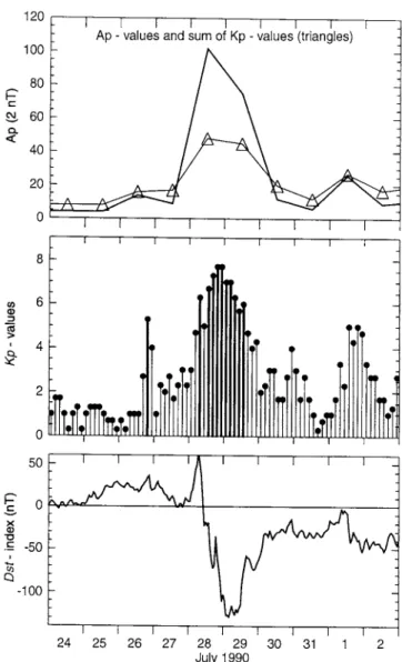
Fig. 1. Geophysical conditions during the time-interval under study

with latitudinal profiles along the orbital track for selected time-moments only, while the incoherent-scatter radar provides plasma parameters of the upper atmosphere for longer time-intervals with good time resolution in a lim-ited region of space. Therefore, the task of combining simultaneous satellite and radar measurements within a common global numerical model can give some insights into the complex physical coupling processes.

2 EISCAT and satellite data for 31 July 1990

The UHF system of the EISCAT radar facility allows three-dimensional measurements of ionospheric para-meters such as electron density Ne, electron temperature ¹e, ion temperature ¹i, ion drift »i, and ion composition at the heights of the D-, E-, and F-layers up to upper ionospheric altitudes of about 600 km. We used the Com-mon Program 1, version I (CP-1-I), registrations from the time-interval 1900 UT 30 July till 0400 UT 01 August 1990, and directed our attention mainly to data taken on day number 212 (31 July 1990) for intercomparison with satellite data from the Active mission. The CP-1 config-uration is intended to provide measurements along the magnetic field line above the Tromsø station (with an inclination of about 77.6° for the flux tube with the Mc-Ilwain parameter ¸"6.46). For this purpose the Tromsø antenna is kept fixed parallel to the magnetic field at 278.5-km altitude and the remote sites take measurements in a 5-min cycle, providing a three-dimensional pattern of the drift velocity in the F region.

The Active mission was launched on 28 September 1989 into a near polar orbit with an inclination of about 82.5°, a perigee of 500 km and an apogee of 2500 km. It consisted of the main satellite Active and the small Czech subsatellite Magion-2, which is able to be stirred, for diagnosis purposes. On 31 July the satellite pair passed nearby the EISCAT radar station during orbit numbers 3805 at 0325 UT and 3812 at 1540 UT. Real-time tele-metry was used so that measurements during overflights above Europe are available. Depending on satellite height these time-series have durations of 15 to 35 min and cover a latitudinal range from about 20° to 80°.

The Czech-Russian ion mass spectrometer HAM-5 (Afonin et al., 1994) used for this study was placed on board the main satellite. It is a three-stage Bennett ana-lyser with electron multiplier operating in the current mode on its output which uses the modulation mode for removing the base flux. The potential of the analyser was floating and controlled by the potential of an isolated probe located near the aperture of the analyser. The mass spectrometer had discrete ranges around the masses 1, 2, 3 and 4, and a continuous range from 6 to 64 amu, all with a constant accelerating voltage and frequency sweep. The mass resolution M/DM (on the level of 10 per cent) was 25. So, concentrations of O`, N`, He`, H` and O``, as well as of molecular ions (at lower altitudes), were obtained along the satellite orbit with a time resolution of about 6 s. The Langmuir probe on-board the subsatellite Magion-2 working in the sweep adaptive voltage regime performs in situ diagnoses of the cold thermal plasma in

the topside ionosphere. It is a cylindrical probe oriented parallel to the geomagnetic field lines, thus it measured mainly field-perpendicular plasma parameters, namely the electron density Ne, electron temperature ¹e and the effec-tive ion mass. The errors of Ne measurements are esti-mated to be less than 10 per cent. The time resolution of the Langmuir-probe measurements along the orbital trace used throughout this paper is 2 s.

3 Geophysical conditions

The period under study is generally characterized by high solar activity near the maximum of the 22nd solar cycle with average values of F10.7 solar radiation around 200. We selected a time-interval near the northern summer solstice when EISCAT observations and satellite passages over the radar station were available. This took place on the third day of the recovery phase of a geomagnetic storm (with peak values of Kp"8~). The observed Ap,

Kp and Dst indices for the period 24 July—2 August 1990

storm was recorded with two sudden storm commence-ments (SSC) at 0108 and 0331 UT on 28 July with a min-imum Dst value of 129 nT at 0400 UT on 29 July 1990. During the night of 28—29 July the three-hourly Ap index reached peak values of 170, but on 31 July these values returned to a quiet-time level around 4 and Kp went down to values between 0` and 2` (see Fig. 1).

In addition, foF2 data from some European ground-based ionosonde stations (Rome, Juliusruh/Ru¨gen, St. Peter Ording, Kaliningrad, Kiew, Loparskaya) were used to obtain a more comprehensive pattern of the geophysi-cal situation. The foF2 values of 31 July from all these stations are near the median values, after some days with strong negative ionospheric storm effects (not shown here). So, one may assume that the ionospheric conditions on 31 July 1990 recovered from the moderate geomagnetic storm two days before.

4 The model GSM TIP

GSM TIP has been described in detail by Namgaladze

et al. (1988, 1990, 1991). It comprises several

computa-tional blocks for the description of the thermosphere, ionosphere, plasmasphere and near-Earth magnetosphere in a height range from 80 km to 15 Earth radii including electromagnetic coupling processes as a single system.

For a given set of input data (possibly time-dependent), the GSM TIP model calculates the time-dependent global three-dimensional structure of the neutral gas temper-ature ¹n, mass density, wind velocity vector Vn and num-ber density of the main neutral gas components N2, O2 and O for the height range 80—520 km by means of numerical integration of the corresponding three-dimen-sional continuity, momentum and heat balance equations in a spherical geomagnetic coordinate system. To reduce the computational efforts, an empirical thermospheric model, such as MSIS-86 (Hedin, 1987), can be used for the calculation of the thermospheric parameters as well, solving only the neutral-gas momentum equation to ob-tain its three-dimensional global circulation. It has been shown by Namgaladze et al. (1994) that the results of self-consistent GSM TIP model runs and GSM TIP mod-elling with the inclusion of the MSIS-86 model are compa-rable in a qualitative manner. A quantitative agreement has been stated there for mid-latitudes and quiet geomag-netic conditions only.

In the lower ionosphere model block the parameters of the E and F1 ionospheric regions are calculated, namely, the total concentration of the molecular ions n(XY`)"

n(NO`)#n(O`

2)#n(N`2), the ion and electron temper-atures ¹i and ¹e and the molecular ion velocity V(X½`) neglecting heat and mass transfer terms. These equations are solved in the same coordinate system as the thermos-pheric block for the height range 80—520 km with the exception of the electron-energy equation, for which the upper boundary is fixed at an altitude of 175 km. These equations are first order in time only, so they require initial values but no boundary conditions.

In the ionospheric-protonospheric module, para-meters of the F2 region of the ionosphere and of the

plasmasphere are calculated, namely, the atomic-oxygen and hydrogen-ion number densities n(O`) and n(H`), as well as ¹i and ¹e, ion velocities V(O`) and V(H`) for the height range from 175 km to the radial distance of 15 Re. We assume that field lines with ¸'15 (¸ parameter of McIlwain) are open. The plasma drift caused by crossed electric and magnetic fields is taken into account. The integration of the continuity, momentum and heat bal-ance equations for the atomic ions is performed along dipole geomagnetic field lines in a magnetic dipole coordi-nate system.

The equation for the potential of the electric field E" !grad(/) is solved in the fourth program module includ-ing the dynamo action of the thermospheric winds and magnetospheric sources via the auroral field-aligned cur-rent system (FACs). The spherical geomagnetic system is used in this block.

The spatial steps of the numerical integration are 10° in geomagnetic latitude for the thermospheric and lower-ionospheric modules, 5° for the lower- ionospheric-protono-spheric and electrical-potential modules, and 15° in the geomagnetic longitude for all groups of the model equa-tions. In the vertical direction the thermospheric code uses 30 non-equidistant grid points between 80- and 520-km altitude which are distributed with step sizes increasing with a geometric progression roughly between 3 and 45 km from the bottom to the top. The ionospheric-protonospheric module (F2 region and plasmasphere) also has variable spatial steps along the magnetic field lines, with step sizes of about 15 km at the lower boundary at 175-km altitude up to several thousand kilometres near the apex of the flux tubes depending on the ¸ value up to a maximum distance of 15 Earth radii. The maximum number of grid points along a given field line is 140. The time integration step is 5 min.

In order to simulate the thermosphere-ionosphere parameters, the GSM TIP requires the following inputs: solar UV and EUV spectra, FACs connecting the iono-sphere with the magnetoiono-sphere, and ionizing particle pre-cipitation patterns and intensities.

Because there are no measurements of the solar EUV fluxes during the year 1990, we have used the technique of Nusinov (1984); it uses a non-linear scaling of the main solar spectral line intensities with the daily and the 81-day averages of F10.7. The variations of the EUV flux observed by the AE-E satellite in 1977—1980 were used for this flux—model. Solar UV fluxes are as the Mount and Rott-man (1983) data.

The ionospheric polar-cap convection pattern is con-trolled by the specific FAC distribution. Region-I and -II FACs (Iijima and Potemra, 1976) in the auroral zone are fixed at constant geomagnetic latitudes of 75° and 65°, respectively. They have been assumed with maximum densities of 2]10~7 A m~2 for region-I and 5] 10~8 A m~2 for region-II currents, which are reached in the 06-18-MLT meridional plane under usual, non-storm conditions.

The electron precipitation patterns in the auroral zone (65°—75° geomagnetic latitude) have been assumed in the following simple form according to precipitation measure-ments typical for average geomagnetic-activity conditions

(cf. Hardy et al., 1985). The soft electron precipitation belts with a characteristic energy of 0.2 keV and an energy flux of &0.2 erg cm~2 s~1 have a Gaussian shape in latitudi-nal direction and were centred around $70° geomagnetic latitude and equally distributed in longitudinal direction. More energetic electron precipitation with E0"3 keV and maximal fluxes of &8.9 erg cm~2 s~1 at 00 MLT have Gaussian distribution forms in latitudinal and longi-tudinal direction. The spectral characteristic of the soft and the energetic precipitating electrons is chosen accord-ing to Maxwellian energy distributions.

In order to calculate correct electron-gas heating rates the photoelectron flux throughout the ionosphere and plasmasphere should be specified accordingly. The calcu-lation of the differential phototelectron fluxes is a rather complex physical and mathematical problem. For our study we have used a simple approximation for the local heating rate of the electron gas in the height range below 600 km by Krinberg (1978) and an analytical expression obtained by Matafonov (1986) for the energy losses of trapped photoelectron fluxes in the plasmasphere (see also Appendix A). These approximations allow us to avoid the solution of the kinetic equations for the photoelectron fluxes in the ionosphere and plasmasphere and ensure an accuracy of the electron-gas heating rate in the order of 20%. But the plasmaspheric heating approximation re-quires as input parameter the maximal escape energy flux of suprathermal electrons into the plasmasphere. This parameter is set to 2]1010 eV cm~2 s~1, which is slightly more than experimental data (Taylor and McPherron, 1974), but is in agreement with theoretical calculations of Krinberg and Tashchilin (1980) obtained for moderate solar activity.

It has been shown by Richards and Torr (1986) and Richards et al. (1986) that vibrationally excited nitrogen N*₂ is very important for solar-maximum conditions in summer. The model considers the strong dependence of the O`-ion loss rate due to N*2 molecules according to the approximation of Pavlov (1986, 1988). A more detailed description is given in Appendix B. The vibrational tem-perature ¹v must be specified for this approximation and has been chosen slightly above the temperature of the neutral gas (Richards and Torr, 1986). Finally, the spatial distribution of the neutral hydrogen gas is important for the charged-particle processes in the upper atmosphere. The concentration of neutral hydrogen in our model was defined similarly to that in the model of Jacchia (1977).

5 Numerical results of modelling

In this study we confine ourselves to comparisons between model results and observations for two selected time-spans around 0325 and 1540 UT when the satellite pair passed nearby the EISCAT station during their orbits 3805 and 3812, respectively. We investigated in particular the sensititvity of model results to changes of the currently worst-known model input parameters: the temperature, ¹v, of the vibrationally excited molecular nitrogen N*2, the ionospheric convection patterns driven by FACs and the suprathermal or photoelectron escape energy fluxes into

the plasmasphere providing thermal electron heating fluxes from the plasmasphere into the ionosphere. The present knowledge about these input parameters is not precise enough, so that one can speculate about their values within reasonable limits in order to guess their effect by comparison with the measurements. These model runs were performed using the MSIS-86 neutral atmo-sphere model within the thermospheric computational block.

5.1 Early-morning calculations, orbit 3805

This subsection describes model results for 0325 UT when the Active satellite pair, during orbit 3805, crossed Central Europe near the EISCAT station. The values of observa-tion are indicated by triangles throughout all the follow-ing figures, which compare EISCAT-measured profiles with modelling results. We used the EISCAT standard 5-min post-integrated parameter fit and produced median values of Ne and ¹e profiles using 12 consecutive standard 5-min intervals around the time of overflight. The mean square deviations of the observed parameters are gener-ally within the size of the used symbol (triangles).

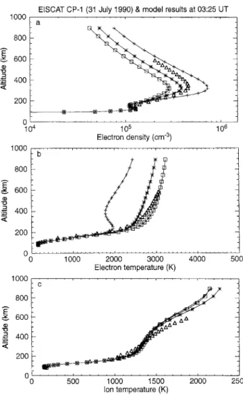
Figure 2a—c demonstrates the effect of varying ¹v, on electron density (a) and electron- (b) and ion-temper-ature (c) profiles above the EISCAT station. The maxi-mum photoelectron escape energy flux is set to 6]1010 eV cm~2 s~1 and the maximum FAC densities are assumed to occur in the 06—18-MLT meridians. The curves indicated by crosses present the model run where N*

2has not been taken into account at all, while the other two cases show results with enhanced vibrational excita-tion of N*

2. The curves marked with asterisks show the case with vibrational temperature ¹v"1.25¹n and the curves marked with squares for ¹v"1.5¹n. From Fig. 2 it is clear that the introduction of N*

2 reduces the Ne F2-peak density dramatically. Comparing the case of ¹v"1.25¹n with the case of ignored N*2, the F2-peak density is reduced by a factor of two. At the same time the electron temperature increases by about 900 K near the F2 maximum at an altitude of 400 km. A further increase in vibrational temperature (¹v"1.5¹n) produces more dramatic changes.

The ion-temperature profiles are close to each other for all cases, especially below 450 km; there the agreement with the EISCAT data is quite good. Above that altitude level the different cases show some small variation and the modelled ¹i begin to deviate from the observed values. This small discrepancy of about 200 K could be caused by insufficient Joule heating, but more likely by adiabatic cooling at high altitude (above 1500 km) due to large plasma escape velocities along the flux tubes in the model results. The high parallel thermal conductivity then results in lower ¹i values down to about 500-km altitude._{The effects of different convection patterns on the local}

Ne, ¹e and ¹i profiles above the EISCAT station are

shown in Fig. 3a—c. As before, the maximum photo-electron escape energy flux is set to 6]1010 eV cm~2 s~1 and model runs with ¹v"1.25¹n are used. We compare different convection patterns which are produced by FAC

Fig. 2.a Electron density, b electron- and c ion-temperature profiles above the EISCAT station for 0325 UT on 31 July 1990; 1-h median values of the measured Ne and ¹e profiles around the time indicated are shown by triangles and are compared with different model results, here, illustrating the effect of N*₂: without including these reactions (curves with crosses), assuming ¹v"1.25¹n (asterisks) and ¹v"1.5¹n (squares)

Fig. 3. As in Fig. 2, but illustrating the effect of different convection patterns; maximum FACs in the 06—18-MLT meridional plane (curves with crosses), 08—20 MLT (asterisks) and 10—22 MLT (squares)

distributions with maximum densities in different meridi-onal sectors. Curves marked by squares show the case where the maximum FACs are reached at 10—22 MLT, while curves with crosses stand for the other extreme with maximum FACs in the 06—18-MLT meridians; curves indicated by asterisks show the intermediate case, i.e. maximum FACs at 08-20 MLT. We see that a clockwise rotation of the maximum FACs from 10—22 to 08—20 MLT leads to a decrease in Ne density and an increase in ¹e, but a further clockwise rotation toward maximum FACs at 06—18 MLT reverses the process and results in an opposite behaviour in the vertical profiles of Ne and ¹e._{As one may notice in Fig. 3c, the ion-temperature} profiles are similiar to the profiles of Fig. 2c below 450 km, but show variations of several hundred degrees above 600 km. These variations are determined in the same way as just shown, by the influence of adiabatic cooling at high altitude due to large parallel escape fluxes.

Figure 4a—c illustrates the effects of varying photo-electron escape energy fluxes on the Ne, ¹e and ¹i profiles above the EISCAT station. Again, the temperature of excited N*

2 was assumed as ¹v"1.25¹n, and the max-imum FACs occured at the 08—20-MLT meridians for these model runs. It can be seen that an increase in the photoelectron escape energy flux from 6]1010 eV cm~2 s~1 (curves with crosses) to 10]1010 eV cm~2 s~1 (squares) leads to a decrease in the electron density mainly in the upper ionosphere and an increase in ¹e at the same heights. From the lower panel (¹i in Fig. 4c) it is clear that the adiabatic cooling effects are even larger than in the previous case (Fig. 3c) due to faster escape velocities.

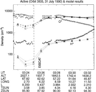
Results from the modelling studies detailed here were also compared with data from the Active satellite orbit 3805 (Figs. 5—7) for upper ionosphere parameters in a latitudinal range from 70° to 45°. The effect of enhanced N*

2 temperatures on the latitudinal distribution of O` and H` is shown in Fig. 5. It can be seen that the O` concentration decreases by a factor of two and the

Fig. 4. As in Fig. 2, but showing the influence of varying photo-electron escape energy fluxes with maximum values of 6]1010 eV cm~2 s~1 (curves with crosses), 7]1010 eV cm~2 s~1 (asterisks) and 10]1010 eV cm~2 s~1 (squares)

Fig. 5. Electron (dots) and ion concentrations along the Active orbit number 3805 for early-morning hours above Europe on 31 July 1990 in comparison with model calculations for different conditions. This figure shows the effect of vibrationally excited N*₂along the orbit as in Fig. 2 for the vertical profiles: without N*₂(curves with crosses), assuming ¹v"1.25¹n (asterisks) and ¹v"1.5¹n (squares). The pas-sage above the EISCAT station is indicated by a dashed vertical line

Fig. 6. As in Fig. 5, but for illustration of the effect of different convection patterns; maximum FACs in the 06—18—MLT meridional plane (curves with crosses), 08—20 MLT (astericks) and 10—22 MLT (squares)

H` density decreases by a factor of 3—4 in the latitudinal range between 70° and 65° if N*

2processes with enhanced ¹v_{The influence of different convection patterns on the}are included. The effect is smaller at mid-latitudes. distribution of O` and H` densities along orbit 3805 (Fig. 6) is similar to that shown in Fig. 3 as far as it concerns oxygen ions. Proton distributions are more sen-sitive to the rotation of the FAC patterns and reach a factor of 5 at the latitude of the EISCAT station. The drift pattern influence has a negligible effect at midlatitudes.

Finally, the ion distributions along the satellite orbit 3805 for various photoelectron escape energy fluxes are shown in Fig. 7. It is clear that the atomic-ion distribu-tions are not sensitive to changes of this input parameter at these latitudes.

5.2 Afternoon calculations, orbit 3812

In this section we present the corresponding numerical results of modelling for the time-span near 1540 UT, when

the satellites passed over the EISCAT station during their orbit 3812. Since the effects of vibrationally excited N*

2are almost identical to the effects at 0325 UT in the morning sector, as presented in Figs. 2 and 5, we concentrate here

Fig. 7. As in Fig. 5, but for the effect of different photoelectron escape energy fluxes as shown already in Fig. 4 for the vertical profiles

Fig. 8. As in Fig. 3, but illustrating the effect of different convection patterns during the afternoon overflight of Magion-2 (orbit 3812) around 1540 UT on 31 July 1990. Here, the variation of the vertical profiles above the EISCAT station are shown for different patterns of convection: maximum FACs in the 06—18-MLT meridional plane (curves with crosses), 08—20-MLT (asterisks) and 10—22 MLT (squares).

on the effects of convection and plasmaspheric heating fluxes.

Figure 8a—c compares the observed and calculated Ne, ¹e and ¹i profiles above the EISCAT station for different patterns of convection for the same cases as in Fig. 3 and with the same assumptions about the photoelectron es-cape energy flux and ¹v. The clockwise rotation of the maximum FACs from 10—22 MLT to 06—18 MLT causes a steady decrease in Ne and an increase in ¹e in accord-ance with the degree of rotation. It should be noted that for these cases Ne and ¹e vary monotonically in contrast to the convection effects in the early-morning sector.

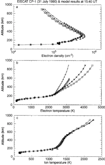
The effect of increasing photoelectron escape energy fluxes on the electron density profiles above EISCAT for the afternoon overflight around 1540 UT is shown in Fig. 9a to be relatively small. In contrast, the electron temperature reacts sensitively to the enhanced heating fluxes from the plasmasphere due to increased photo-electron escape energy fluxes (Fig. 9b). The agreement between measured and modelled ion temperatures is very good for all cases during the afternoon (cf. Figs. 8c and 9c). Changes to the convection and photoelectron escape energy fluxes also have small effects on the ion distribu-tions along satellite orbit number 3812 at low and mid-latitudes. Therefore, we show only the influence of excited N*

2on the electron-density distribution along the satellite orbit in Fig. 10. For this case the maximum FACs were in the 06—18-MLT meridional plane and the photoelectron escape energy flux was set to 2]1010 eV cm~2 s~1 for all latitudes except along the flux tube above the EISCAT station, where a value of 6]1010 eV cm~2 s~1 was as-sumed. It can be seen that the effect of vibrationally excited N*

2 is different at different latitudes and its effect has an upper limit of a factor of 1.5.

6 Discussion

In the previous section we presented numerical model results obtained with the inclusion of the MSIS-86 neu-tral-atmosphere model and compared them with observa-tions from EISCAT for two different local times (dawn and dusk) and with satellite data from the same time-spans but obtained over a certain latitudinal range. Since not all of the input model parameters can be determined correctly from experimental data, we have chosen three essential parameters, such as enhanced N*

2 temperature ¹v, photoelectron escape energy fluxes and maximum FAC locations, to adjust their values accordingly to bring model results and measurements into agreement. We showed that the effect of introducing enhanced N*

2on the modelled vertical Ne and ¹e profiles above EISCAT are very large for both dawn (0325 UT, Fig. 2) and dusk (1540

Fig. 9. As in Fig. 8, but showing the influence of varying photo-electron escape energy fluxes with maximum values of 6]1010 eV cm~2 s~1 (curves with crosses), 7]1010 eV cm~2 s~1 (asterisks) and 10]1010 eV cm~2 s~1 (squares)

Fig. 10. As in Fig. 5, for comparison of model results with measured electron density values obtained on-board Magion-2 (Langmuir probe) along the satellite orbit 3812. The effect of vibrationally excited N*₂is investigated: without N*₂(curves with crosses), assum-ing ¹v"1.25¹n (asterisks) and ¹v"1.5¹n (squares)

UT) sectors. The decreases in Ne density at F2-peak alti-tudes varies from a factor of 2 in the dawn sector to a factor of 3 in the post-noon sector. In these cases, lower ¹evalues correspond to higher Ne, and vice versa. A tem-perature difference of more than 1000 K is predicted at 400-km altitude between the case of absent N*

2 and the other extreme (including N*_{2with ¹v"1.5¹n). This result} agrees with the model results of Ennis et al. (1995) for maximum solar activity in summer at mid-latitudes.

The convection electric fields have an important effect on ionospheric parameters at high latitudes, but the cor-rect inclusion of this effect requires knowledge of the plasma convection over the entire high-latitude region. Unfortunately, we have no complete experimental data about the convection during this period of interest, since data from EISCAT radar alone are insufficient to deter-mine the electric field over the entire high-latitude region; Rasmussen et al. (1986) have been faced with the same problem. Therefore, we varied the normal position of the maximum FACs (06—18 MLT) by rotating the meridional plane of maximum currents to calculate the electric-field

distribution of ionospheric convection in the high-latitude region. In all these cases the model results have shown a two-cell convection with anti-sunward flow over the polar cap and return flow at lower latitudes (Fig. 11a—c). The cross-polar-cap potential drop varies weakly between 22.5 kV (Fig. 11b), 25.0 kV (Fig. 11a) and 27.5 kV (Fig. 11c). But at the same time the cross-polar electric field vector points in different directions: approximately from 04 to 16 MLT in the first case (a), 06—18 MLT in the second (b) and nearly 09—21 MLT in the last case (c). The effects of the rotated convection patterns on Ne and ¹e are different for the dawn and dusk sectors, but generally smaller than the effects of vibrationally excited N2. The changes in Ne due to different convection patterns above EISCAT are about 50% near the F2 peak and about 600—700 K for ¹e. As can be seen in Fig. 3a, the model gives remarkably good agreement between Ne profiles above EISCAT and model results in the dawn sector when the maximum FACs are in the 10—22-MLT meridional plane and equally good agreement in the dusk sector when the maximum FACs are in the 08—20-MLT plane (Fig. 8a). However, the ¹e values are lower than EISCAT measurements in both cases.

Figure 12a—c show the eastward and northward com-ponents of the modelled electric field (left panels) and a comparison between the calculated meridional neutral wind with the corresponding values from the empirical HWM93 model for all three different convection patterns (a—c), adopted in our study. It can be seen that the clock-wise rotation of the maximum FACs from 10—22 MLT to 06—18 MLT leads to a variation of the maximum values of both electric-field components and to slight changes of the meridional neutral-wind component. We use this figure

Fig. 11a–c. Electric-field-potential (kV) distribution at the northern hemisphere in a geomagnetic latitude/longitude frame with ortho-graphic projection for three different FAC patterns: a maximum FACs in the 06—18-MLT, b 08—20-MLT c and 10—22-MLT meridi-onal plane. The location of the EISCAT station for the two different time-moments is indicated by triangles

for an explanation of the behaviour of the vertical

Ne profiles presented in Figs. 3 and 8 from the previous

sections.

As we saw in Fig. 3, the rotation of the maximum FACs causes a non-regular behaviour of the Ne profiles over EISCAT. The effect can be explained by the non-regular variations of the northward electric field component

En (west-east drift). We see that En changes from

!7 mV m~1 for the case with FACs maximum in the 10—22-MLT plane (case c) to !9 mV m~1 in the 08—20-MLT case (b) and !8 mV m~1 in the 06—18-MLT case (a, cf. Fig. 12). So, En has its maximal negative value in the dawn sector for case b with FACs maximum in the 08—20 MLT plane and hence during the maximal zonal plasma drift from the night sector towards the morning sector.

The meridional wind (positive southward) contributes to an uplifting of the F2 layer, especially for the cases b and c (maximum FACs from 8—20 to 10—22 MLT).

During the overflights in the dusk sector (1540 UT), the meridional neutral wind component is near zero and the behaviour of the F2-peak electron concentration is deter-mined by the electric-field components only. As we saw in Fig. 8, the Ne concentration and the height of the F2-layer increase with the rotation of the maximum FACs from the 6—18-MLT plane to 10—22 MLT. This is caused by the eastward electric-field component Ee, which varies around 1540 UT from !3 mV m~1 to #3 mV m~1 for the different cases. The eastward electric-field component causes a meridional plasma drift, and hence acts to push ions up (as in case c) or down (case a) along the magnetic

Fig. 12a–c. Eastward- and northward-electric-field components versus UT (left panels) and the meridional neutral wind velocity at an altitude of 300 km in comparison with the HWM93-model

wind at the location of EISCAT (right panels) for the three cases of different FAC patterns: a maximum FACs in the 06—18-MLT, b 08—20-MLT and c 10—22-MLT meridional planes

field lines towards regions of lower or higher chemical loss rates, respectively. The zonal plasma drift (En) does not change its direction in all these cases.

An inspection of the right panels of Fig. 12a—c shows that the agreement between the modelled meridional wind velocities and the corresponding values from the HWM93 empirical wind model is quite good. This is valid espe-cially near the time-moments of our interest in the dawn and dusk sectors.

The influence of the electron heating flux on upper ionospheric parameters, simulated in this study by the specification of the photoelectron escape energy fluxes, is more pronounced during dawn than in the dusk sector. In the dusk sector, as seen in Fig. 9a (1540 UT), the model variability of Ne profiles is only around 20%, while the photoelectron escape energy fluxes vary from 6]1010 eV cm~2 s~1 to 10]1010 eV cm~2 s~1. But in the same time ¹e increases appreciably from 2500 to 3200 K at 400-km altitude (Fig. 9b). Figure 9a reveals also, that the model Ne concentrations reproduce the observed vertical profiles above about 350 km (at least for the case with a flux of 6]1010 eV cm~2 s~1), but underestimate

the electron density below this altitude. An increasing heating flux results in only a small decrease of the

Ne density above 350 km, and has practically no influence

below this level.

In the dawn sector, as seen in Fig. 4a for 0325 UT, the model Ne concentration appreciably underestimates the electron density above 250 km. This difference becomes larger with increasing photoelectron escape energy fluxes, especially above 500 km.

The discrepancies of these effects in the dusk and dawn sectors can be explained by the plasma drift along mag-netic field lines, induced by the combined effects of ambi-polar diffusion and neutral-wind drag. In the dusk sector, the neutral-wind is directed to the north, while in the dawn sector the neutral wind points in the opposite direc-tion. So, the escaping thermal plasma flow in the dusk sector is lower than in the dawn sector for nearly equal electron temperatures. It may be noted that the influence of electron heating fluxes from the plasmasphere on the electron density profiles of the upper ionosphere are small in the dusk sector but have a pronounced effect above 400 km in the dawn sector.

The model results for Ne and ¹e profiles above EIS-CAT, as discussed up to this point, are obviously not unambiguously determined by the model input data set for the period under study. In order to obtain more precise information about the temporal-spatial distribution of the ionospheric parameters and to decrease the input data uncertainties involved in the modelling, we have used experimental data from the Active mission for the same time-periods.

A comparision of the Ne measurements along the or-bital track of the subsatellite Magion-2 with the model results is shown in Fig. 10. As already stated, the effects of convection and electron heating fluxes from the plasma-sphere for this time-interval are unimportant at mid-lati-tudes and they will not be presented here. But the vibrationally excited N*

2has an appreciable influence on

Ne and ¹e for all latitudes. The photoelectron escape

energy fluxes at mid-latitudes were assumed with 2]1010 eV cm~2 s~1 in this case. As can be seen in Fig. 10, the model tends to overestimate the Ne concentration along orbit 3812, when N*

2 was not taken into account, and it has a reasonable agreement for the case with ¹v"1.25¹n. Thus, if we accept that during quiet geomag-netic conditions the spatial distribution of Ne concentra-tion has no sudden latitude-longitude changes, we may assume that ¹v"1.25¹n is a reasonable value for all latitudes, including the EISCAT location. The assumption is quite reasonable, especially for our conditions of high solar activity in summer when the main ionospheric trough is absent.

Comparisions with atomic-ion concentrations along the Active orbital track with model results for orbit 3805 near 0325 UT are shown in Figs. 5—7. A good agreement between model and experimental data can be noticed for the case of ignored N*

2 (Fig. 5). In the case with ¹v"1.25¹n, the O` and H` concentrations are de-creased. This effect is more prominent for the H` density at the latitudinal range from 60° to 70°. A further increase in ¹v causes a larger decrease in the atomic-ion concentra-tions in the high-latitude range.

The effects of different convection patterns on the atomic-ion density along orbit 3805 and the comparision with experimental data are shown in Fig. 6. It can be seen that a reasonable agreement between model results and orbital data at high latitudes are achieved for the cases with maximum FACs in the 10—22 MLT and 06—18-MLT meridional planes. It should be noted that a reasonable agreement was obtained between Ne profiles over EIS-CAT and also model results for the same convection (Fig. 3).

Finally, the effects of different photoelectron escape energy fluxes on the O` and H` model concentrations along the orbit 3805 are also small, as can be seen in Fig. 7. But they show marked plasma-density depletions and ¹e increases near the EISCAT station where the fluxes were enhanced artificially. This is an effect of the thermal plasma outflow which is close to the regime of the polar wind above 1000 km. The upward proton flux depletes the H` density while affecting the O` density profile through its scale height. The latter process increases the O` scale height to the plasma scale height, which is larger than the

individual O` scale height. Thus, the decrease of the O` concentration at 400—500 km altitude does not lead to an appreciable depletion of the O` density at 2000-km altitude. A more detailed explanation of this effect can be found, for example, in the paper of Blelly et al. (1992).

Thus, as indicated in Figs. 5—6, the case without vibrationally excited N*

2 and a convection with max-imum FACs reached in the 06—18-MLT plane is more preferable with regard to the experimental data of orbit 3805. But we should keep in mind that the model runs with ¹v"1.25¹n and the same convection pattern also give a reasonable agreement between model and orbital data.

7 Summary and conclusions

In this work we have made an effort to take advantage of the global thermosphere-ionosphere-plasmasphere model (GSM TIP) for the interpretation of the experimental data sets obtained for the same time-spans but separated in space. At the same time the study provided reliable inputs to the model by a reasonable matching of numerical model results with the experimental data sets obtained from three different sources: two orbits of the Active mission and CP-1 observations from the EISCAT station on day 212 (31 July) of 1990.

The satellite pair passed near the EISCAT station around 0325 and 1540 UT at an altitude of about 2000 and 2200 km, respectively, and the satellite data (Ne, ¹e and ion composition) were obtained onboard the Ac-tive main satellite and its subsatellite Magion-2. The peri-od under study is generally characterized by high solar activity near the maximum of the 22nd solar cycle with an average value of F10.7 of the solar radiation around 200._{The numerical model calculations were performed by} using the MSIS-86 neutral-atmosphere parameters and with consideration of vibrationally excited nitrogen mole-cules.

Since one cannot derive all model inputs directly from experimental data for the period under study, we studied the influence of three main input parameters: the temper-ature of the vibrationally excited N*

2, the convection electric-field patterns resulting from different FAC distributions and the photoelectron escape energy flux. They were adjusted to the observed values to provide a best fit. We obtained similarities between model behav-iour on one side and satellite and EISCAT data on the other.

The detailed comparisons between the experimental data and the numerical model results have shown that the most preferable case can be obtained with the following model inputs set: the inclusion of N*

2 with ¹v"1.25¹n, maximum FACs reached at the 06—18-MLT meridional plane and a photoelectron escape energy flux of 6]1010 eV cm~2 s~1 over EISCAT and 2]1010 eV cm~2 s~1 for all other latitudes.

For these inputs, the electron density profiles above EISCAT are in qualitative agreement with the model results both at 0325 and 1540 UT, but the model Ne con-centration is a little lower (about 15 to 20 per cent) than

the EISCAT data. The comparision of the electron-tem-perature measurements with the model calculations at 0325 and 1540 UT for the same case has shown, in general, a good agreement as well, although the model tends to underestimate the ¹e values for both time-spans by about 100—200 K. The good agreement between the model meri-dional neutral-wind component and the corresponding values of the HWM93 empirical wind model for the EIS-CAT location supports the conclusions drawn.

The comparision of the model Ne density along the Magion-2 orbital track 3812 with measured values has shown that the case with ¹v"1.25¹n is a good choice, providing a reasonable agreement between model and satellite data at all latitudes and confirming the result obtained for the EISCAT station at 1540 UT.

The measurements of O` and H` concentrations ob-tained in the dawn sector (0325 UT) by the Active main satellite show by comparison with the model results that the assumed convection pattern with maximum FACs in the 06—18-MLT meridional plane and the selected photo-electron escape energy flux of 6]1010 eV cm~2 s~1 are good input data, but an even better agreement was ob-tained if vibrationally excited N*

2 was not taken into account for this case. The inclusion of N*

2 in the model calculations with ¹v"1.25¹n causes a decrease in the O` and H` density in the high-latitude region by a factor of nearly two for H` and 20% for O`, which is the main component at this altitude.

It should be noted here that all these discrepancies between model results and experimental data are related to various uncertainties involved in the modelling of the ionospheric situation under study and may be eliminated by some slight variation of the input data.

The sensitivity of the model results to the variation of three main input data has been studied in this work in detail. We found that the inclusion of vibrationally excited N*

2 is very important for the period under study. The

Ne density at F2-region altitudes changes by a factor of

2 or more if one includes N*

2; while the sensitivity of the density profile with respect to changed convection and electron heating flux variations from the plasmasphere is less pronounced and shows different behaviour at the dawn and dusk sectors.

Thus we conclude that the normal ionospheric convec-tion pattern corresponding to quiet geomagnetic condi-tions obtained with maximum FACs reached in the 06—18 MLT plane are correct for these time-spans in the dawn and dusk sector. The inclusion of vibrationally excited N*

2 in the model calculations is very important and the values of the excited N*

2temperature are near ¹v&1.25¹n. With respect to mid-latitudes, an enhanced photo-electron escape energy flux is required above the EISCAT station. Their values were assumed to be 2]1010 eV cm~2 s~1 and 6]1010 eV cm~2 s~1, respectively. It is possible that there is another significant source of heat for electrons of the upper ionosphere and plasmasphere, but the limited experimental data base makes it difficult to determine unequivocally what is physically taking place.

Acknowledgements. This work was supported by the Deutsche Agentur fu¨r Raumfahrtangelegenheiten (DARA) under grant 50 QL

92060. We are grateful to K. Schlegel (MPAE, Lindau-Katlenburg) for providing EISCAT data, to F. S. Bessarab for assistance with the graffic data reduction and to N. S. Natsvalyan for fruitful discussions on numerical methods during the code development.

Topical Editor D. Alcayde´ thanks P.-L. Blelly and G. Millward for their help in evaluating this paper.

References

Afonin, V. V., K. V. Grechnev, V. A. Ershova, O. Z. Roste, N. F. Smirnova, J. A. Shultschishin, and J. Smilauer, The ion composi-tion and ionosphere temperatures in the maximum of 22/$ cycle of solar activity as measured on board of ‘‘Intercosmos-24’’ (project Active) satellite (in Russian), Kosm. Issled., 32, 82—94, 1994.

Blelly, P. L., D. Alcayde, M. Blanc, and J. Fontanari, Thermal polar wind: Opportunities with the EISCAT Svalbard radar, Ann. Geophysicae, 10, 498—510, 1992.

Ennis, A. E., G. J. Bailey, and R. J. Moffett, Vibrational nitrogen concentration in the ionosphere and its dependence on season and solar cycle, Ann. Geophysicae, 13, 1164—1171, 1995. Fuller-Rowell, T. J., D. Rees, S. Quegan, R. J. Moffett, and G. J.

Bailey, Interactions between neutral thermospheric composition and the polar ionosphere using a coupled ionosphere-thermo-sphere model, J. Geophys. Res., 92(A7), 7744—7748, 1987. Hardy, D. A., M. S. Gussenhoven, and E. A. Holeman, A statistical

model of auroral electron precipitation, J. Geophys. Res., 90(5), 4229—4248, 1985.

Hedin, A. E., MSIS-86 thermospheric model, J. Geophys. Res., 92(A5), 4649—4662, 1987.

Iijima, T., and T. A. Potemra, The amplitude distribution of the field-aligned currents at northern high latitudes observed by TRIAD, J. Geophys. Res., 81, 2165—2174, 1976.

Jacchia, L. G., Thermospheric temperature, density and composi-tion: New models, SAO Spherical Report, No. 375, 1977. Krinberg, I. A., Kinetics of the electrons in ionosphere and

plasma-sphere of the Earth (in Russian), Nauka, Moscow, 1978. Krinberg, I. A., and A. V. Tashchilin, The influence of the

ionosphere-plasmasphere coupling upon the latitude variations of the iono-sphere parameters, Ann. Geophysicae, 36(4), 537—548, 1980. Matafonov, G. K., Distribution of energy losses of photoelectrons

between ionosphere and plasmasphere (in Russian), Issled. Geomagn. Aeron. Fiz. Solntsa, 75, 73—78, 1986.

Moffett, R. J., G. H. Millward, S. Quegan, A. D. Aylward, and T. J. Fuller-Rowell, Results from a coupled model of the thermo-sphere, ionosphere and plasmasphere (CTIPM), Adv. Space Res., 18, (3)33—(3)39, 1996.

Mount, G. H., and G. J. Rottman, The solar absolute spectral irradiance 1150—3173 A_{s : May 17, 1982, J. Geophys. Res., 88(9),} 5403—5410, 1983.

Namgaladze, A. A., Y. N. Korenkov, V. V. Klimenko, I. V. Karpov, F. S. Bessarab, V. A. Surotkin, T. A. Glushchenko, and N. M. Naumova, Global model of the thermosphere-ionosphere-protonosphere system, Pure Appl. Geophys. 127(2/3), 219—254, 1988.

Namgaladze, A. A., Y. N. Korenkov, V. V. Klimenko, I. V. Karpov, F. S. Bessarab, V. A. Surotkin, T. A. Glushchenko, and N. M. Naumova, A global numerical model of the thermosphere, iono-sphere, and protonosphere of the earth (English translation), Geomagn. Aeron., 30(4), 515—521, 1990.

Namgaladze, A. A., Y. N. Korenkov, V. V. Klimenko, I. V. Karpov, V. A. Surotkin, and N. M. Naumova, Numerical modelling of the thermosphere-ionosphere-protonosphere system, J. Atmos. ¹err. Phys., 53(11/12), 1113—1124, 1991.

Namgaladze, A. A., Y. N. Korenkov, V. V. Klimenko, I. V. Karpov, F. S. Bessarab, V. M. Smertin, and V. A. Surotkin, Numerical modelling of the global coupling processes in the near-earth space environment, in Proc. 1992 Symp./5th COSPAR Colloq., Ed. D. N. e. a. Baker, Vol. 5, Washington Pergamon Press, pp 807—811, 1994.

Namgaladze, A. A., O. V. Martynenko, A. N. Namgaladze, M. A. Volkov, Y. N. Korenkov, V. V. Klimenko, I. V. Karpov, and F. S. Bessarab, Numerical simulation of an ionospheric disturbance over EISCAT using a global ionospheric model, J. Atmos. ¹err. Phys., 58(1—4), 297—306, 1996.

Nusinov, A. A., Dependence of intensity of lines of shortwave radi-ation of the sun on activity level (in Russian), Geomagn. Aeron., 24(4), 529—536, 1984.

Pavlov, A. V., The reaction rate coefficient for O` with oscillatory excited N2 in the ionosphere (in Russian), Geomagn. Aeron., 26(1), 152—154, 1986.

Pavlov, A. V., The role of vibrationally excited nitrogen in the ionosphere, Pure Appl. Geophys., 127(2/3), 529—544, 1988. Rasmussen, C. E., R. W. Schunk, J. J. Sojka, V. B. Wickwar, O. De

La Beaujadiere, J. Foster, J. Holt, D. S. Evans, and E. Nielsen, Comparison of simultaneous Chatanika and Millstone Hill ob-servations with ionospheric model predictions, J. Geophys. Res., 91(A6), 6986—6998, 1986.

Richards, P. G., and D. G. Torr, A factor of 2 reduction in theoretical F2 peak electron density due to enhanced vibrational excitation of N2 in summer at solar maximum, J. Geophys. Res., 91(A10), 11331—11336, 1986.

Richards, P. G., D. G. Torr, and W. A. Abdou, Effects of vibrational enhancement of N2 on the cooling rate of ionospheric thermal electrons, J. Geophys. Res., 91(A1) 304—310, 1986.

Richmond, A. D., E. C. Ridley, and R. G. Roble, A thermosphere/ ionosphere general circulation model with coupled elec-trodynamics, Geophys. Res. ¸ett., 19(6), 601—604, 1992. Roble, R. G., and E. C. Ridley, A thermosphere-ionosphere-meso

sphere-electrodynamics general circulation model (TIME-GCM): Equinox solar cycle minimum simulations (30—500 km), Geophys. Res. ¸ett., 21(6), 417—420, 1994.

St.-Maurice, J.-P., and D. G. Torr, Nonthermal rate coefficients in the ionosphere: The reactions of O` with N2, O2 and NO, J. Geophys. Res., 83(3), 969—977, 1978.

Stubbe, P., and W. S. Varnum, Electron energy transfer rates in the ionosphere, Planet. Space Sci., 20, 1121—1126, 1972.

Taylor, G. N., and P. H. McPherron, Diurnal and seasonal vari-ations of exospheric heat flux at a mid-latitude station, J. Atmos. ¹_{err. Phys., 36(7), 1135—1146, 1974.}

Appendix A: heating by photoelectrons

Heating rates of the electron gas are calculated using the following analytic formulas.

Qe(s)"Qel(s)#Qenl(s), (A1) where Qel is the local heating rate and Qenl the non-local heating rate. The local heating rate is calculated by the well-known formula Qel(s)"eqe(s), (A2) wheree is efficiency of the local heating electron gas, and qe(s) is the photoionization rate. The efficiency has been taken according to Krinberg (1978) in the following form

e"0.16[9#lg(Ne(s)/Nn(s))]2 [eV]. (A3) Here Ne(s) is the electron concentration and Nn is the sum of neutral-particle concentration. The non-local heating rate is approxi-mated by the following analytical formula according to Matafonov

(1986) Qenl(s)"Qt(s)_B0(s)B(s)_:S0Ne(s) ~S0Ne(s)ds , (A4) with Qt(s)"q0(s)

G

A

B

A

BH

Appendix B: vibrationally excited nitrogen

Effects of vibrationally excited molecular nitrogen (N*₂) on the electron concentration are carried out by means of the loss-rate variation for O` ions in the reaction

O`#N*2"NO`#N. (B1) The rate coefficientb for this reaction without taking into account N*₂ is given by the well-known formula of St.-Maurice and Torr (1978). A correction of this rate coefficient for N*₂is made in corre-spondence with the works of Pavlov (1986, 1988) in the following way. Let us consider the effective rate coefficientb* as

b*"i/=+ i/0

biNi

+Ni, (B2)

wherebi are the rate coefficients of reaction B1 for the ith excited level of N2 with a number density Ni; b0 is the rate coefficient without consideration of N*₂. The coefficientsbi for the first, second and third vibrational levels can be written as

bi"Ai¹n#Bi , (B3) where

Ai"3.391]10~15; 2.234]10~14; 3.022]10~14 K~1 cm3s~1, and

Bi"3.722]10~13; 3.085]10~11; 1.921]10~10 cm3 s~1.

¹n is the temperature of the neutral gas. For a Boltzmann distribu-tion we get

Ni

+ Ni"(1!exp(!3353/¹v)) exp(!3353i/¹v), i51, (B4) where ¹v is the temperature of N*2. The main cooling rate of the electron gas by N*₂was calculated using the formula of Stubbe and Varnum (1972).