Biopsy-Implantable Chemical Sensor
byChristophoros C. Vassiliou
S.B. Electrical Science and Engineering, MIT, 2004
M.Eng. Electrical Engineering and Computer Science, MIT, 2006 Submitted to the
Department of Electrical Engineering and Computer Science in partial fulfillment of the requirements for the degree of
Doctor of Philosophy at the
MASSACHUSETTS INSTITUTE OF TECHNOLOGY
rAAIVE
'I
September 2013
©
Massachusetts Institute of Technology 2013. All rights reserved.Author...
Department of Electrical Engineing and Computer Science August 30, 2013
Certified by ...
..
.w
...Michael J. Cima David H. Koch Professor of Engineering Thesis Supervisor
Biopsy-Implantable Chemical Sensor
by
Christophoros C. Vassiliou
Submitted to the
Department of Electrical Engineering and Computer Science on August 30, 2013, in partial fulfillment of the
requirements for the degree of Doctor of Philosophy
Abstract
There is a dire need for tools that can rapidly detect cancer treatment efficacy. A cancer patient must endure the side effects of chemotherapy and radiotherapy. It will be weeks before a change in the size of the tumor can be observed and the oncologist has the information necessary to determine whether treatment is working. Valuable time is lost searching for the right treatment and the right dose.
This thesis presents a sensor that can be implanted inside the body during a biopsy procedure and wirelessly report on the tissue environment. The sensor has direct
access and can track metabolic markers, such as pH and oxygen, which have been shown to predict outcome, dose, and response to cancer treatment. These markers cannot be measured anywhere else except directly inside the tissue, and this sensor provides that access. The probe allows for repeat, non-invasive measurement of the same location after the initial biopsy.
The sensor consists of a small nuclear magnetic resonance (NMR) probe that has a cavity filled with a contrast agent sensitive to the chemical of interest. An NMR relaxation measurement of the contrast agent reveals the chemical concentration. Wireless NMR measurements are performed with the aid of a reader probe that resides outside of the body. The reader generates the excitation pulses and receives the NMR signal. The sensor and reader have a mutual inductance that enables the
and eliminates any signal from the surrounding tissue. The coupled reader-sensor performs standard NMR relaxation measurements. A method is presented to produce the sensors in large numbers, and the sensors are tested in vivo.
The probe is designed to be implanted during a routine procedure and would be no more invasive than existing clinical practice. The measurements can track tumor progression and guide therapy before any physical changes can be observed, and the
patient can receive the right treatment as soon as possible.
Thesis Supervisor: Michael J. Cima
Acknowledgments
I am truly grateful to my advisor, Professor Michael Cima. I joined his lab as an
undergraduate and have had the opportunity to work on a number of projects. The breadth of research topics in his lab and the number of departments that have been represented in the lab are a testament to his boundless energy and fearless approach to science and engineering. He has taught me to ask the right questions and inspired me to tackle seemingly insurmountable problems, seeking solutions that draw from diverse fields. I look forward to our future collaborations.
I am thankful for Professor Sangeeta Bhatia and Professor Elfar Adalsteinsson for
their service on my thesis committee. I am grateful for their advice regarding my personal and career development, and I am certain that those lessons will continue to benefit me for many years to come.
I have benefited from the guidance and mentorship of Professor Isaac Chuang, who
has offered many helpful suggestions and recommendations throughout my graduate career. I am grateful to the Course VI Graduate Office and to Janet Fischer, in particular, for her patience.
Funding for this research was provided by the National Cancer Institute, the National Science Foundation, and the United States Air Force.
I have had the good fortune of being in a lab with a group of amazing individuals
whose greatest strength is their willingness and ability to work together. The lab members have been a second family to me and I truly enjoyed the time I've spent in
Many thanks to the other members of the project: Yibo Ling, Vincent Liu, and Syed Imaad. I will always remember our many hours in the lab, our trips to Billerica and Burlington, and our conversations about nothing in between scans in the imaging suite. I am indebted to you for your contributions to the project, and I could not have asked for a better group of people to work with. I look forward to seeing how the project evolves with the newest member Gregory Ekchian. I was fortunate to have had the opportunity to work with an amazing undergraduate researcher, Melanie Adams. Special thanks to Byron Masi with whom I shared countless hours in the machine shop. Many, many thanks to you all for your camaraderie and friendship: Hong Linh, Heejin, Yoda, Dan, Alex, Noel, Maple, Qunya, Jen, Urvashi, Kevin, Jay,
Jack, Negar, Joan, Matt, Laura, Ndria, Katerina, and Lina. Thanks to Milton for assistance with the machining. I am truly thankful for all the hard work that Barbara Layne and Lenny Rigione put in to keep the lab running and us out of trouble.
I enjoyed working with our collaborators through the CCNE project, and especially
Keith Brown, Dave Issadore, and Professor Westervelt at Harvard University. Thank you also to Elizabeth, Rachel, and Greg for helpful comments and suggestions that improved this manuscript.
I have benefited greatly from the amazing staff and resources at the Koch Institute,
and I am especially thankful for the help of Scott Malstrom and Milton Cornwall-Bradley. I would also like to thank Alex Fiorentino for the many outreach opportu-nities.
at the Edgerton Student Shop. And many thanks to the members of DCM for their assistance and training. Thank you to my many MIT friends but especially Krish, Robin, Laura, Daanish, and Ted.
I am truly thankful for my Mom and Dad, Hariclea and Christakis, who encouraged my early interest in science and engineering and whose sacrifices ensured that my siblings and I received the best possible education. Thank you to my in-laws, Judy and Paul, for their support and assistance throughout and especially for their help with errands during crunch time.
Finally, I would like to express my sincere gratitude to my wife and best friend, Elizabeth. Her enthusiasm, wit, and humor have seen me through my graduate degree. She is my champion and cheerleader, and I am a better person because of her. This is as much her achievement as it is my own.
I dedicate this thesis
in memory of our beloved children, Angeliki and Panagiotis,
Contents
1 The clinical need
1.1 Sensors inside the body . . . . 1.2 Cancer . . . . 1.2.1 Treatment . . . . 1.2.2 New drug approvals . . . .
1.2.3 The tumor microenvironment
1.3 Thesis overview . . . .
2 Background
2.1 Nuclear Magnetic Resonance
2.1.1 Signal strength . . . . 2.1.2 Relaxation . . . . 27 . . . . 27 . . . . 30 . . . . 30 . . . . 32 . . . . 33 . . . . 34 37 . . . . 38 . . . . 38 . . . . 4 1
2.3 M utual Induction . . . .
3 Wireless NMR
3.1 Magnetic field amplification ...
3.2 Circuit model . . . . 3.2.1 Transmit mode . ... 3.2.2 Receive mode . . . . . 3.3 Design considerations . . . . . 3.3.1 Sensor length . . . . . 3.3.2 Wire diameter . . . . . 3.3.3 Sensor diameter . . . .
3.3.4 Reader coil diameter .
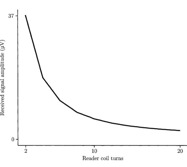
3.3.5 Number of turns on the
3.3.6 Noise and EMI . . . . 3.3.7 Reader coil length . . .
3.3.8 Tissue conductivity . . 3.4 Practical considerations . . . 3.4.1 Tuning frequency . . . 54 59 59 reader coil . . . . 62 . . . . 64 . . . . 68 . . . . 73 . . . . 73 . . . . 74 . . . . 75 . . . . 79 . . . . 79 . . . . 83 . . . . 84 . . . . 84 . . . . 86 . . . . 89
3.5 Sensor fabrication
3.6
3.7
3.8
3.5.1 Machining the plastic body .
3.5.2 Winding the coil . . . .
3.5.3 Tuning the resonant circuit . 3.5.4 Potting in epoxy . . . .
3.5.5 Filling with the assay material Reader fabrication . . . . Testing the complete system . . . . . Conclusion . . . .
4 Oxygen sensing
4.1 Oxygen and cancer therapy 4.2 Oxygen as a contrast agent . . . 4.3 Oxygen sensitivity . . . . 4.4 Oxygen sensitivity experiments 4.5 Tissue oxygen measurements .
4.5.1 Inspired oxygen... 4.5.2 Restriction of circulation . . . . 98 . . . 10 1 . . . 10 1 . . . 10 2 . . . 104 . . . 104 . . . 10 5 . . . 10 7 111 . . . 112 . . . 113 . . . 116 . . . 118 . . . 118 . . . 12 1 . . . 12 1 95
5 pH sensing
5.1 Electrochemical pH sensors . . . .
5.2 HEMA-BIS gels for pH measurements. . .
5.3 Temperature dependence . . . .
5.4 Pilot study . . . . 5.5 Detecting chemotherapeutic efficacy . . . .
5.6 Conclusion and future work . . . .
6 Detecting protein biomarkers
6.1 Cardiac biomarkers . . . .
6.1.1 Exposure . . . . 6.1.2 Mouse myocardial infarction model
6.1.3 Future cardiac sensor applications .
6.2 Nanoparticle aggregation . . . . 6.3 Prospects . . . . 127 . . . 128 . . . 129 . . . 132 . . . 136 . . . 138 . . . 142 145 . . . 147 . . . 148 . . . 148 . . . 152 . . . 154 . . . 164 7 Conclusion
A Least-squares echo estimation
A .1 T heory . . . .
165
173
B Numerical computation of mutual inductance
Bibliography 189
List of Figures
1-1 Biopsy implantable NMR sensor ... 35
2-1 Transverse relaxation is measured using the CPMG pulse sequence.
A 900 pulse rotates the magnetization into the x - y plane. A train
of refocusing pulses compensates for field inhomogeneities and the signal appears as brief "echoes". The envelope of the echo amplitudes (dashed) decays with a time constant, T2. . . . . 43 2-2 Saturation Recovery measures the longitudinal, or spin-lattice
relax-ation. A burst of pulses with decreasing intervals completely sat-urate the magnetization such that the net is zero. The system is allowed to recover for a time tau during which the z-directed mag-netization approaches the equilibrium magmag-netization, Mo. The relax-ation is interrupted with a spin-echo sequence to generate an echo
with M(T) = Mo(1 - eT/IT). The relaxation time, T, is measured by
2-3 Plate format NMR (left) combines a commercially-available
single-sided NMR probe with a 3-axis robot. The NMR MOUSE measures a thin slice above the surface thanks to its unconventional magnet arrangement shown on the right. . . . . 47 2-4 An RLC circuit models the capacitor-inductor circuit with the resistor
representing the losses in the inductor. At very low frequency the resistance is R, while at high frequency the capacitor shorts out the
current source. . . . . 48
2-5 Response of the RLC circuit to a current input . . . . 49
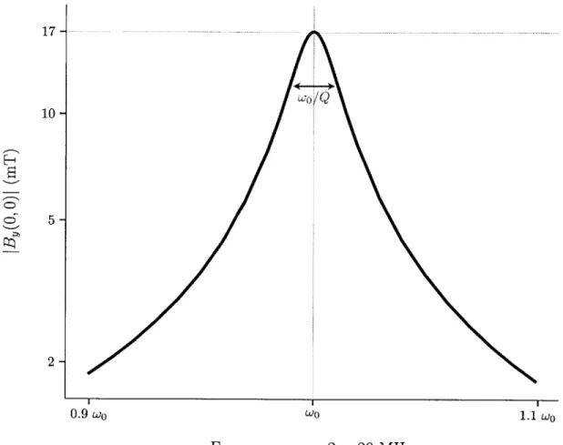
2-6 Frequency response of an RLC circuit . . . . 51
2-7 Two dimensional simulation of magnetic field in cylindrical coordinates Y- . A 20 turn coil is modeled with 1 A current flow. The field lines show the direction of B, and the color represents the magnitude of the
y directed field. . . . . 52
2-8 Two dimensional cross section of current distribution. The images are
cylindrically symmetric about the left side of the page. The coil has a larger resistance at high frequency because the current flows mostly on the inner surface of the coil. . . . . 53 2-9 Mutual inductance represented in a circuit diagram. . . . . 54 2-10 The field generated by a changing current in one coil induces a voltage,
3-2 The field generated inside the sensor is greatly enhanced when the
sensor is excited at the resonance frequency by a current flowing in the reader coil. . . . . 63 3-3 Transmit path showing a 50 Q voltage source connected to the reader
probe. The resistors model losses in the coils. . . . . 65
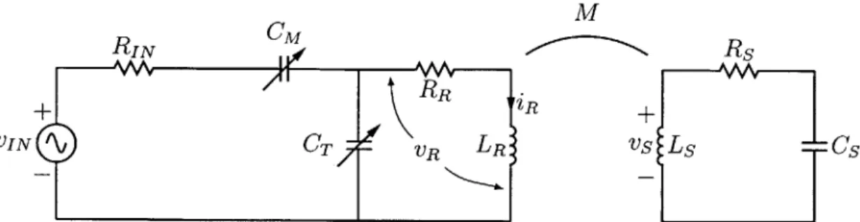
3-4 Block diagram of the coupled probes. Solution of the feedback loop gives the current in the sensor coil. . . . . 65 3-5 Simplified transmit path with the admittance YCp representing the
couple reader-sensor. A single-coil NMR probe has YCp = (R + jwL)- 1. 67 3-6 Simulation of the field inside the sensor coil as a function of distance
from the reader coil. A tuned reader coil increases the field inside the sensor coil more than 20 fold. . . . . 69 3-7 Signal reception path. The NMR signal appears as a voltage across
the sensor coil. Resistive losses in the coils are modeled as noise sources. 70
3-8 A tuned reader coil ensures enhanced reception of the NMR signal. . 72
3-9 Field map of sensor coil showing high degree of uniformity in the
sample chamber. The contour lines represent M.,/Mo, the projection onto the transverse plane following a 900 pulse calibrated to the center of the cham ber. . . . . 74
3-10 The signal-to-noise ratio as the wire diameter is increased. The
small-est possible wire diameter will maximize the signal-to-noise by increas-ing the sample volume. The coil length is fixed and the wire is wound as compactly as possible; many more turns of the finer wire are needed to fill the length. . . . . 76 3-11 Photograph of sensors with smaller diameter coil and chamber to
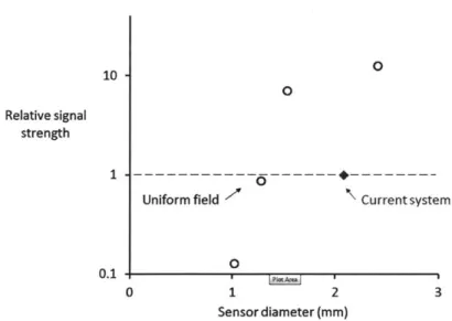
in-vestigate the practical lower limit on sensor size. . . . . 77 3-12 Signal strength versus sensor diameter normalized to the 2.2 mm
sen-sor on the single-sided magnet. The largest sensen-sor for a given appli-cation gives the strongest signal. . . . . 77 3-13 Simulated signal-to-noise ratio versus sensor diameter. Increasing the
sensor volume increases the signal-to-noise ratio, but the gains are modest as the sensor becomes very large. . . . . 78
3-14 The received signal amplitude decreases as the number of turns on the reader coil is increased. . . . . 80 3-15 Thermal noise at the receiver due to losses in the reader and sensor
coils. The thermal noise from the reader coil dominates the sensor coil noise when the reader coil has fewer than six turns. If thermal noise is the only noise source then the reader coil should be designed so that the sensor noise is dominant. . . . . 81 3-16 Considering only the thermal noise, the signal-to-noise ratio increases
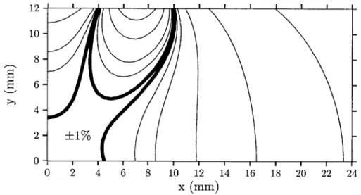
3-17 Mutual inductance between a two-turn reader coil and a sensor coil
versus position. The diagram is rotationally symmetric about the ^ direction. The thick line represents the volume over which M changes less than 1% from the origin. . . . . 85 3-18 Mutual inductance contour map when the two turns of the reader coil
are separated by one radius. The 1% region is significantly expanded compared to Figure 3-17. . . . . 85 3-19 The field strength inside the sensor is virtually unchanged over the
range of conductivity expected inside the body. The increased resis-tance of the reader coil captures the loss in the conductive medium. . 87 3-20 Plot of sensor field versus the conductivity of the surrounding medium.
Higher frequency operation is generally preferred except in very high conductivity m edia. . . . . 88 3-21 Plot of signal-to-noise ratio as a function of mismatch between the
sensor resonant frequency and the Larmor frequency. Maximum SNR is achieved on resonance, but slight deviations in the sensor's resonant frequency do not matter. . . . . 89 3-22 The reader coil can be tuned to a lower frequency without the sensor
to maximize the signal-to-noise ratio when the sensor is inserted. The SNR is equivalent to tuning at the resonant frequency with the sensor inside. This method provides a way to tune when the precise location of the sensor is unknown. . . . . 91
3-23 Measured echo amplitude versus the angle between the reader and
sensor axes. The signal is relatively insensitive to angular deviations less than 20' and is detectable even with deviations as large as 60*. . 92
3-24 Field strength inside the sensor at a distance from the reader coil mimics the human system configuration. A larger radius coil improves the sensitivity at larger distances. There is an optimum coil radius for each measurement depth. . . . . 94
3-25 Photograph of an implantable sensor . . . . 95
3-26 Core biopsy needle. A trocar facilitates insertion into the body. The
cannula provides a channel through which the biopsy needle can obtain multiple tissue samples . . . . 96 3-27 Sensor implantation following a mock biopsy procedure on a gelatin
phantom . . . . . 97 3-28 Subcutaneous implantation needle. . . . . 98
3-29 Key components of implantable sensor . . . . 99
3-30 Machining the sensor body and cavity. The cavity is drilled (1-2) and
the coil support bobbin are milled using carbide end mills (3). The lower portion will house the capacitor and is cut to the final sensor diam eter (4). . . . 100 3-31 Machining the capacitor pocket. The stock is rotated 900, and a pocket
3-32 Photograph of a completed NMR probe. A sensor is made by filling
the chamber with the appropriate chemically sensitive contrast agent. 103
3-33 Complete measurement apparatus for preclinical testing. . . . 106
3-34 Verifying the measurement of an echo and scaling with pulse
ampli-tude. The maximum echo amplitude represents the 900 condition. . . 107 3-35 Transverse relaxation measurement acquired with an implanted sensor. 108
4-1 The oxygen sensor response (top) to changing oxygen fraction in a balance of nitrogen (bottom). Each condition was maintained for
30 min. A saturation pulse sequence with 600 ms recovery time yields
a very fast Ti-weighted intensity measurement for monitoring dynamics. 119 4-2 Calibration curve of T weighted intensity versus oxygen fraction in
nitrogen. The error bars are smaller than the marker size. . . . 120
4-3 Boxplot of T measured by a sensor implanted in a rat calf muscle. The inspired gas was changed from oxygen to air, and an increase in T followed. A second transition back to oxygen did not show a corresponding difference. A longer time might be needed for the recovery. . . . 122 4-4 T measured in a calf muscle under free and constricted circulation. A
significant increase in relaxation time is observed after applying light pressure to the thigh. . . . 124
5-1 Measurements of T2 versus pH of a saline solution using HEMA-BIS
gel inside a sensor. A peristaltic pump maintained a constant flow of saline from a temperature controlled bath over the device. A pH
probe in the bath monitored both temperature and pH. . . . 131
5-2 T2 versus pH calibration curve. . . . 133 5-3 Histogram of pH measurement error establishing a limit of detection
better than 0.1 pH units. . . . 134 5-4 The measured T2 decreases with temperature. The expected
temper-ature deviation in vivo is very narrow compared to the studied range,
but the calibration curve must be performed at body temperature. . . 135 5-5 Relaxation time measurement for sensors implanted inside, near, and
contralaterally to the tumor. The sensors on the tumor side measured a shorter T2, consistent with a lower tissue pH. . . . 137 5-6 Measured relaxation times for sensors implanted in mouse tumors.
Those animal receiving treatment (doxorubicin) are shown as solid red lines, and the control group that received saline injections are shown in dashed black lines. Each line represents a different animal. No discernible pattern emerges between the two groups suggesting that this dose had no effect on the tumor pH. . . . 140
5-7 Measured relaxation times for implanted sensors that received no
im-5-8 Histologic section of an untreated tumor (H&E stain). Significant
re-gions of necrotic tissue are mostly stained pink. Healthy melanoma cells have purple-stained nuclei. The brown spots are melanin, char-acteristic of melanoma. . . . 142
5-9 H&E stained sections of treated and untreated tumors. Substantial
regions of necrotic tissue (pink with no purple stained nuclei) are ap-parent in both sections. . . . 143
6-1 Prototype device used to test protein detection. Sensitive
nanoparti-cles are encapsulated in a plastic body using a semipermeable mem-brane that keeps the nanoparticles in but allows the target to pass.
... 146
6-2 Antibody based sensors measure exposure, defined as the time integral
of concentration. Transient events can be detected because exposure remains high even after the concentration has subsided. . . . 149
6-3 Measured T2 versus time. Sensors exposed to steady concentrations of
myoglobin respond at different rates but saturate to the same value. Adapted from Ling, Pong, Vassiliou et al. [89]. . . . 150 6-4 Measured T2 versus myoglobin exposure. The measurements from
Figure 6-3 all lie along a characteristic T2 vs exposure curve. Transient
profiles (markers) simulate one-off events and also lie along the curve. Adapted from Ling, Pong, Vassiliou et al. [89]. . . . 151
6-5 Sensors implanted in a myocardial infarction (MI) model. MRI
mea-surements of the sensor (a) show one possible use. Sham and control experiments show that the sensors indeed detect the MI (b). The mea-sured T2 increase with the amount of damaged tissue (c-e) as would be expected from Figure 6-4. Reproduced from Ling, Pong, Vassiliou et al. [89]. . . . 153
6-6 Scanning electron micrograph of 1 pm beads. . . . 155
6-7 A tube containing particles suspended in molten agarose is inserted
into a weak magnetic field. The particles begin to form chains. A water-cooled jacket gels the agar solution after a predetermined time, and the particle formation is captured. . . . 156
6-8 Bright field transmission micrograph of 1 iim beads suspended in agar. The chains were created by magnetizing the sample using an electro-magnet (B=4mT). . . . 156
6-9 The average chain length determined by optical imaging shows a
power-law increase with time inside the 4 mT magnetic field. . . . 157
6-10 The tube is rotated along an axis perpendicular to instrument field, BO, with 0, being the angle between particle chains and BO. . . . 158
6-11 Relaxation time measurements as a function of angle between the magnetized direction, B and the measurement field direction, BO. . . 159 6-12 Measured relaxation time as a function of magnetization time shows
6-13 The difference between high and low T2 values as the sample is rotated
relative to the magnetic field also increases as a function of magneti-zation time and chain length. . . . 161 6-14 Isosurfaces of field perturbations caused by a three-particle chain at
different angles to the field. The top and bottom surfaces (red) bound the 1% positive field deviation, and the center, torroidal surface (blue) bounds the negative 1% field deviation. The shape and volume of the
1% boundaries change with angle and are responsible for the angular
dependence of T2. . . 162
6-15 The volume of solution for which the field is perturbed at least 1% is
shown versus chain angle and normalized to the particle volume. The three-particle chains show a gentler field gradient consistent with an increasing T2. Rotating the chain 900 increases the field gradient, and
a shorter T2 is expected. . . . 163
7-1 Concept implantable sensor for simultaneous pH and oxygen measure-m ents. . . . 170
A-1 Typical signal acquired from one echo. The echo envelope is formed by summing multiple echoes at the start of a multi-echo sequence. . 177
A-2 The signal-to-noise ratio of the least squares estimate increases as more
data is acquired. Increasing the integration time eventually adds noise but no data and leads to a reduction in SNR. . . . 179
A-4 Plot of the maximum achievable signal-to-noise ratio versus the re-ceiver phase angle. The integral method requires phase alignment, but the least squares method gives an optimal SNR regardless of phase angle. . . . 181
A-5 The echo envelope changes over the first few echoes. . . . 182
A-6 Normalized signal amplitude for echoes 5 to 100. The echo shape is
List of Tables
2.1 Simulation parameters and outputs for a 20-turn coil. . . . . 54
4.1 Siloxane molecule physical parameters and interaction with oxygen. The values are used in Equation (4.2) to estimate T. . . . 115 4.2 Measured and predicted values of T for siloxanes in air. The
sensi-tivity is ultimately determined by the very high inherent T values of the material .. . . . 115
5.1 Acquisition parameters for measuring the transverse relaxation time, T 2. . . . 136
Chapter 1
The clinical need
Sensors implanted inside the body offer the medical practitioner a unique vantage point. They provide direct access to the physical and chemical environment of the tissue that blood tests and imaging do not offer. Needle probes provide similar access but are too invasive for routine and repeat use. This thesis presents a sensor designed to be implanted during a biopsy procedure and to wirelessly report on its surround-ings. The sensor performs repeat virtual biopsies on the same site using contrast agents developed for magnetic resonance imaging (MRI) to measure proteins, oxy-gen, and pH. This sensor is demonstrated primarily as a tool for monitoring cancer but also finds applications in heart disease and traumatic injury.
other means, in a timely manner, and with minimal patient discomfort. These consti-tute the sensor engineer's guiding principles. The usefulness of a sensor is measured
by how its availability changes clinical practice. Before building a sensor the engineer
should ask, "Will clinicians do anything differently based on this sensor's readings?" This question is best answered in conversation with a practicing clinician.
The discussion with the clinician is also critical to determine where the sensor will reside and how it will be deployed. All existing procedures in the standard of care offer avenues for deploying a sensor. The chosen avenue will also constrain the device's design. If key-hole surgery is performed with laparoscopic tools then the device must be designed to fit through those tools. Designing for existing procedures makes the deployment method obvious to a doctor or surgeon; it fits in neatly with their current practice. The existing procedures also offer a method of payment since reimbursement codes are already in the system. Avoiding additional procedures reduces the risk to the patient and the overall cost of care.
How fast the sensor must measure depends on the application. An implantable defibrillator must continuously monitor heart activity by taking measurements many times per second. It does this to take necessary corrective action when abnormal cardiac rhythms are detected. The information must be acted on immediately and while the patient may be incapacitated. The direct monitoring enables the life-saving instrument[1]. A sensor that tries to detect whether cancer therapy is working only needs to measure once a day or less. Measuring every second will not add any information, since no changes occur on that time-scale. The decision on how often to sample influences how the device is powered and, consequently, how big the device
made smaller than commercially available medical batteries[2].
The PillCam is a small battery operated camera that exemplifies the importance of patient comfort. It is swallowed and travels along the 9m tortuous path of the digestive system taking photographs along the way[3, 41. It transmits the images to a belt worn by the patient. The doctor receives a complete view of the GI tract within one or two days. The imaging is done at home and avoids having to schedule an endoscopy or colonoscopy. It has farther reach than either of those procedures and is incomparably more comfortable. It is no surprise that it is finding uses for diagnosing many types of gastrointestinal conditions.
There has been no discussion of science or engineering so far, because the most important decision is what a sensor or device should do to provide the most benefit to the patient. The technology is secondary; even the most technologically advanced sensor is useless if it provides no meaningful information or if it will never be used. The first decision is what the device should do, and then it is up to the engineer to choose the best tool for the job.
The sensor presented in this thesis is designed to monitor cancer directly from within a tumor. It measures clinically relevant markers that may indicate how the tumor is progressing and whether therapy is proving effective. It takes weeks of treatment for changes in the size of a tumor to manifest; changes in pH inside the tumor have been detected as early as one day after treatment. The sensor response time, measured in minutes and hours, is much faster than any anticipated change inside the tumor. Designed to be implanted during a biopsy procedure, the sensor fits nicely into clinical
1.2
Cancer
Worldwide, 7.5 million people died from cancer in 2008. That year approximately
12.7 million people were diagnosed with cancer. Cancers of the lung, breast and
colorectum made up one third of the total[5]. This year, in the United States alone, over 1.6 million people will be diagnosed with cancer[6]. It can be expected that the global diagnosis figure will rise dramatically as screening improves in developing
nations and more cases are detected.
Fortunately the number of cancer survivors is also increasing. Patient education and better screening have lead to earlier detection and treatment[7]. There were over
13 million cancer survivors at the start of 2012; that number is expected to reach 19 million in the next decade[8]. Lesions are discovered through self-examination,
routine screening, and imaging. A cancer diagnosis, however, is almost exclusively confirmed by a direct observation of the suspected tissue, that is, by biopsy[9]. A needle biopsy is an invasive medical procedure that removes a small tissue sample from inside the body. A pathologist microscopically examines the cells to look for cancerous cells. The findings also help identify the type of cancer, which will point to a particular course of therapy that is most likely to succeed. Treatment can involve radiotherapy, chemotherapy, and/or surgery.
1.2.1
Treatment
proliferate by evading the body's mechanisms for dealing with misbehaving cells. They co-opt blood vessels to provide perfusion necessary for growth and eventually escape from the tumor to invade the rest of the body[10, 11, 12]. The rapid rates of cell division and genetic mutation make treatment very hard, and resistance develops quickly even to treatments that were initially effective.
High rates of morbidity are associated with treating cancer. Many of the side effects are not from the disease but from the treatment. Patients undergoing chemotherapy or radiotherapy will likely experience fatigue, emotional distress, and severe pain[8].
Radiation therapy and surgery have fewer side effects because the treatment is lo-calized, but tissue around the targeted area is still susceptible to damage.
Chemotherapy causes widespread damage to the body leaving no tissue unharmed; every system is adversely affected. The list of side effects mirrors the list of tissues and organs in the body. Chemotherapy reduces white blood counts, suppressing the immune system and increasing the risk of secondary infections. The drugs damage tissue throughout the digestive system, beginning in the mouth and gums, down the throat, and along the lining of the intestines. The compromised digestive system causes malnutrition and dehydration. Nausea and constipation are also common side effects that compound these problems. The brain, skin, lungs, hair follicles, and the peripheral nervous system are all adversely affected. Cardiotoxicity and decreased bone density are major concerns. Add extreme fatigue and sleep disruption to this, and it is not hard to see why over half of cancer patients experience severe emotional distress[8]. These adverse effects are accepted because chemotherapy does more damage to cancer cells than to healthy cells and because there are no other
dosage must be found early on to reduce the overall morbidity and prevent metastasis, which is responsible for 80 % of all cancer related deaths[10]. Many drugs are effective only for a small fraction of patients, and identifying the right drug for a patient is an entire area of research[9]. It may be weeks after the treatment starts before doctors can determine whether the drug is working or not. A sensor that directly monitors a tumor could quickly and definitively assess response thus saving critical time in the early stages of the disease.
1.2.2
New drug approvals
Recent drug approvals by the Food and Drug Administration (FDA) highlight the dire need for methods to determine whether a drug is working or not. Four re-cently approved drugs achieved less than 6 months increase in median survival with overall response rates well below 50% of the treated population. The drugs only modestly improve over previously approved drugs and some carry the potential for serious toxicity in the heart and liver. Detecting treatment efficacy is extremely important.
The human epidermal growth factor receptor 2 (HER2) is expressed in a third of breast cancer patients and is predictive of poor reponse to therapy[13]. However, the receptor can be targeted by antibodies and is the basis for several drugs. The response rate to trastuzumab is 30% among HER2 positive patients compared with just 9% across all patients. Added to chemotherapy it increased median survival from 20 to 25 months[10]. Among the 2013 drug approvals is ado-trastuzumab
there is an enormous benefit to identifying HER2 positive patients, but even among this preselected population more than half of the patients will not respond. While the newer drug may perform better across a patient population, there is no way of knowing whether an individual patient will respond or not.
Regorafenib is a new drug for treating metastatic colorectal cancer[17]. It was ap-proved despite only increasing survival by 1.4 months with a response rate of 5%. The justification of approval in the summary review is telling, "While the absolute magnitude of the treatment effects on survival [...] are small, the ability of any single agent to demonstrate efficacy in this heavily pre-treated population represents clinical benefit" [18].
This particular drug has relatively mild side effects, but that is not always the case. Identifying the patients who are responding ensures that only those who are benefit-ing are subjected to the side effects. A sensor could identify the 60% of HER2 positive patients that aren't responding and reduce their risk of severe hepatic and cardiac toxicity. If efficacy is detected quickly, then the 9% of HER2 negative patients who might benefit from trastuzumab can be identified.
1.2.3
The tumor microenvironment
Cancer is more than just a collection of cells but behaves as an organ in which the sur-rounding environment is as important as the constituent cells[19]. The extracellular matrix, once thought to be a collection of cell-binding proteins, is increasingly being recognized as an important contributor to the tumor lifecycle[10, 20]. It is actively
growth pattern of a tumor depends on the three dimensional arrangement of its consituent cells[22]. A study on individual cells found that cells confined to a 20 pm diameter post were likely to die but cells given a 50 pm plot continued to grow[23]. This raises the possibility of new treatments that target the tumor microenvironment and not just the cells[24].
Cells removed from the body provide only part of the story. Cell morphology, gene mutations, and surface protein expression tell only half the story. One can envision that tumors will be characterized also by properties of tumor environment such as oxygen, pH, and vascularization. Studying the tumor environment should be as important as studying the response of cells in a culture dish. An oncologist with feedback from a sensor inside the tumor could quickly try multiple drugs, identify the one most likely to work, and start the patient on the right drug as soon as possible. The disease will be treated sooner, and the patient will be spared the side effects of ineffective treatment.
1.3
Thesis overview
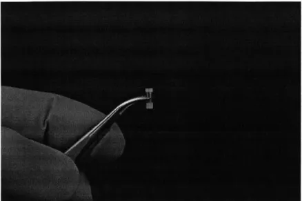
This thesis presents an implantable NMR probe (figure 1-1) that can be implanted directly inside a tumor using a standard biopsy needle. A variety of NMR contrast agents are used to create sensors for oxygen, pH, and various proteins. The on-board circuit enhances the signal strength, allows wireless remote measurement, and eliminates any interfering signals from the surrounding tissue. The sensors exploit nuclear magnetic resonance (NMR) for measurement. Chapter 2 provides a brief
Figure 1-1: Biopsy implantable NMR sensor
ical framework and the design and construction of an implantable NMR probe. The sensors rely on contrast agents to convert a chemical concentration or dose into an NMR signal, and several examples are presented. Chapter 4 demonstrates on oxy-gen sensor and tests it in a rat model. These measurements can predict the efficacy of chemotherapy and radiotherapy. Chapter 5 presents a pH sensor for monitoring the acidic environment of a tumor tested in a melanoma model in mice. Decreasing
pH following chemotherapy has been proposed as an indicator of treatment efficacy.
Chapter 6 shows how protein biomarkers can be measured as sentinels for myocardial tissue damage caused by myocardial infarction or chemotherapy induced cardiotox-ity. The prospects for human use are discussed in Chapter 7 along with additional work needed to bring this to fruition.
Chapter 2
Background
The sensor is comprised of a wireless nuclear magnetic resonance (NMR) probe that contains a chemically sensitive contrast agent. NMR is not an obvious choice for a miniaturized sensor because the signal is extremely weak compared to other tech-niques. However, it offers an array of contrast mechanisms, and NMR can be per-formed on opaque media and through tissue. Optical sensors require clean, trans-parent samples. Optical detection through tissue is hindered by severe absorption and scattering. Ionizing radiation (X-ray) or radioactive sources (positron emission tomography) are unacceptable for repeat monitoring, while ultrasound lacks contrast and chemical sensitivity. Overall NMR is an excellent modality for sensors inside the body.
A wireless NMR probe is discussed in detail in Chapter 3. This chapter introduces
res-2.1
Nuclear Magnetic Resonance
This thesis deals with a classical description of 'H NMR as introduced by Bloch[25]. This approach is acceptable because 1H is a spin-1/2 system, all samples are at high temperature (300 K), and each sample contains approximately 1020 spins. The net magnetization is not quantized, but rather a vector that can be manipulated with an alternating magnetic field. Almost every NMR book includes the classical description and derivation. A good overview is presented by Cowan[26]. Fukushima and Roeder give substantial practical advice on building NMR probes[27]. Slichter's text covers a graduate course on NMR[28], and the classic text by Abragam[29] is a complete treatise on all aspects of NMR theory. Important papers by Hoult and Richards present a clear method for determining the signal strength in an NMR experiment [30,
31] and a description of the NMR receiver[32]. The articles in the journal Concepts in Magnetic Resonance[33, 34] are written from a pedagogical perspective, covering all
aspects of NMR. New research can be found in the Journal of Magnetic Resonance[35] and Magnetic Resonance in Medicine[36].
2.1.1
Signal strength
NMR requires a magnetic field, BO = BOZ, created either with permanent magnets or
with superconducting coils in spectrometers and imaging systems (MRI). Convention defines the direction of the field as 2 and refers to the 2-^ plane as the transverse plane.
rotated by means of an oscillating magnetic field, B1 (t), that is perpendicular to the
static field, BO, and at a specific frequency called the Larmor frequency, wo = ^1Bo.
The constant of proportionality, 7, is the gyromagnetic ratio and depends on the nucleus. Hydrogen, specifically 1H, has a gyromagnetic ratio of 2.675 x 10⁸ s-1'T-1 or 42.57MHz T-1. The nuclear magnetization of a small sample with spin number I = in a magnetic field, BO, is given by,
MO= ' 2h2 NB (2.1)
2kB T
where the sample contains N protons at a temperature, T; h is the reduced Planck constant; and kB is the Boltzman constant. Equation (2.1) gives clear guidance on increasing the magnetization: increase the sample size, increase the field strength, and lower the temperature. An implantable sensor goes against all of these. The sensor must be small, the remote measurement limits the field strength, and the temperature is fixed at 37 C. It is these constraints on the sample that require an on board circuit.
An oscillating field applied perpendicularly to 2, such as,
B1(t) = B1 sin(wot) , (2.2)
perturbs the nuclear magnetization, M, away from equilibrium. The transverse component, Mx = M x 2, will precess around 2 at a frequency equal to the Larmor
sin(wot). A rotating reference frame is applied such that the oscillating field can be described only by its time-varying magnitude and a phase term. The oscillating field is turned on momentarily and rotates M at a rate, w, = ^yB1, around the x axis.
The angle of rotation,
#,
is given by#
= wit = -yBit (2.3)Two useful pulses are those that rotate the magnetization by 900 and 1800. The first rotates the magnetization onto the transverse plane and satisfies the condition
'yBitgo = 7r/2. The second condition is simply twice the pulse area, -yBltiso = r, and
rotates the magnetization into the negative longitudinal direction, M = -MO.
The component of the magnetization in the transverse plane precesses around Z and induces a voltage in a loop of wire around the sample. Faraday's law of induction states that the voltage is proportional to the time rate of change of the magnetic flux. Conveniently, the magnetic flux can be calculated by, MoiB1, where b1 is the
magnetic field at the sample generated by unit current through the loop[31].The induced voltage is
VNMR = wOMo51 (2.4)
where the frequency factor, wo, is due to the time derivative of the oscillating magnetization [30]. This voltage will be measured by the coil, and the coil design is also important. A wire loop carrying unit current has a magnetic field at the center equal to
f51 = PO (2.5)
The underlying assumptions are that the sample is uniform, the magnetic field is constant, and the oscillating field is also of uniform magnitude. A spherical sample in a long coil would certainly qualify. A small coil completely filled with sample will have regions of lower field near the ends that cannot be ignored. The signal can be calculated by first dividing the sample into many smaller samples. Each sample is assumed to be uniform, and the contribution from each will be summed to give the overall signal.
2.1.2
Relaxation
Various mechanisms are responsible for how the magnetization returns to equilib-rium after it has been perturbed with the oscillating field[39, 40]. Two relaxation time constants appear in Bloch's equations and are referred to as the spin-lattice or longitudinal relaxation time, T1, and the spin-spin or transverse relaxation time,
T2. When a sample is initially placed in a magnetic field, the nuclear magnetization
develops over time as follows:
A(t)
= ZMO (1 - e/T1). (2.6)A 900 pulse rotates the magnetization into the transverse plane, so M,, = MO and Mz = 0. The transverse component decays towards zero and is given by
There is an assumption of a perfectly homogeneous magnetic field, but in reality this is rarely the case. Slight variations in the magnetic field across the sample result in a spatially varying Larmor frequency. If a 900 pulse is applied along X at time, t = 0, the magnetization is rotated into the ^ direction. The precession continues
for a brief period of time, r. If the field variation across the sample is AB, then a phase variation develops equal to
AO = yTAB. (2.8)
Hahn discovered that applying a 1800 pulse in this state could correct for this deviation[41]. This 'refocusing pulse' effectively multiplies the phase by minus one. The fastest precessing regions that had gained phase +# now have phase -0 and vice versa for the slowest regions. The phase continues to accumulate, and at a time t = 2r there will be no phase variation across the sample. This momentary construc-tive interference is detected as an 'echo' by the receiver. Carr and Purcell extended this work to allow for a train of pulses and echoes to measure relaxation time[42]. Meiboom and Gill modified this to eliminate compounding errors due to imperfec-tions in the oscillating field[43]. The CPMG sequence is used almost exclusively in systems with inhomogeneous fields and is shown schematically in figure 2-1. If the initial 900 pulse is along X then the 180' pulses are alternately applied along +9 and
-Y. This ensures that any imperfections in the oscillating field do not accumulate from one echo to the next. The peak of each echo is stored, and the decaying envelope gives the material's inherent relaxation rate. Appendix A discusses an acquisition
pulses
echo time
signal - ~
Figure 2-1: Transverse relaxation is measured using the CPMG pulse sequence. A
900 pulse rotates the magnetization into the x - y plane. A train of refocusing pulses
compensates for field inhomogeneities and the signal appears as brief "echoes". The envelope of the echo amplitudes (dashed) decays with a time constant, T2.
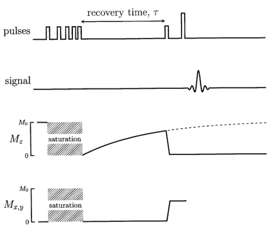
Measuring longitudinal relaxation requires a different set of pulse sequences. The nuclear magnetization is orders of magnitude smaller than the applied field and so it is preferable to rotate the magnetization into the transverse plane for detection. Saturation recovery is the preferred method for measuring T on systems with a grossly inhomogeneous magnetic field, such as the NMR-MOUSE[44, 45]. The se-quence starts with a series of pulses that saturate the magnetization such that the net magnetization equals zero. The magnetization is allowed to recover for a time, T, at which point a spin-echo method is applied to measure M,(T). The sequence, shown in figure 2-2, is repeated for several different recovery times, and the full relaxation profile is acquired. Multiple echoes can be acquire, instead of just one, using the CPMG pulse sequence. This improves the estimate of M(T)[46].
Contaminants in a sample that perturb the field in their immediate vicinity can increase the relaxation rate. These contaminants could be regions of different
per-recovery time, T
pulses
signal Mo ---Mo M , saturation 0-Figure 2-2: Saturation Recovery measures the longitudinal, or spin-lattice relaxation.
A burst of pulses with decreasing intervals completely saturate the magnetization such that the net is zero. The system is allowed to recover for a time tau during which the z-directed magnetization approaches the equilibrium magnetization, MO. The relaxation is interrupted with a spin-echo sequence to generate an echo with
M(r) = Mo(1 - e-/T1). The relaxation time, T1, is measured by repeating the sequence for different recovery times.
The relaxation-concentration curves can be used as sensors. Magnetic nanoparticles tagged with antibodies form the basis of the contrast agents used in Chapter 6 for measuring soluble protein biomarkers. Chapter 4 deals with an oxygen sensor that exploits relaxation induced by paramagnetic oxygen in solution. Chemical exchange is a process by which hydrogen atoms on a polymer can be exchanged with hydro-gen atoms on nearby water molecules. The rate of exchange is pH dependent and influences the measured relaxation rate. A relaxation-pH relationship arises that is used as a pH sensor in Chapter 5. The mechanisms are discussed in their respective chapters.
2.1.3
Hardware
Typically, in pulsed NMR, a single coil generates an oscillating magnetic field to manipulate the nuclear magnetization and also detects the NMR signal. A radio frequency (RF) switch inside the NMR spectrometer (KEA2, Magritek) alternately connects the coil to a power amplifier to generate the pulses and to a sensitive preamplifier to receive the echoes. The pulses typically last less than 10% of the overall duration allowing ample time for the oscillation to die down and for the switch to connect the preamplifier to detect the NMR signal[26, 27].
Two permanent-magnet systems are used in the experiments described here. A benchtop relaxometer (Minispec mq-20, Bruker) is used for testing samples in stan-dard 5 mm glass tubes. The samples are inserted through a port in the top of the instrument and sits between two magnets. The arrangement creates a relatively
Zealand) that measures samples that are outside the instrument. The field, which runs parallel to the surface, decreases with distance away from the surface. The sensitive region is a flat sheet of sample approximately 250 Pm thick. This magnet is particularly useful for measuring samples that won't fit into a traditional instrument. The magnet arrangement is shown in the cutaway view in figure 2-3. The field has a built in field gradient that allows the slice selective measurement. However, this gradient adversely affects the transverse relaxation measurements. Molecules diffusing along the direction of the gradient experience a changing Larmor frequency and a random accumulation of phase. The CPMG sequence cannot fully compensate for this phase accumulation, and the measured T2 is significantly lower than on a
homogeneous field magnet.
The figure also shows a rapid NMR screening system, dubbed the AutoNMR, that is designed to measure samples in standard plate format. A modular frame connected to a 3-axis motion stage allows for up to 168 samples to be measured sequentially. A circulating water bath maintains a constant magnet temperature to avoid a drift in the field strength over the course of a day. Custom software controls the robot and programs the pulse sequences.
2.2
Resonant Circuits
It is merely coincidence that a resonant circuit is used to detect the nuclear magnetic resonance signal. An untuned coil can measure the signal, but a circuit with a
b
Rare earth magnets
Irc
Figure 2-3: Plate format NMR (left) combines a commercially-available single-sided NMR probe with a 3-axis robot. The NMR MOUSE measures a thin slice above the surface thanks to its unconventional magnet arrangement shown on the right.
A capacitor, C, is connected with an inductor, L, in series as shown in figure 2-4. A
resistor, R, captures the resistance of the inductor. This RLC circuit has a resonant frequency,
WO (2.9)
VLOU
A sinusoidal driving current at the resonant frequency, i(t) = sin wt, will cause
R
iL
T_
C=
7
L
Figure 2-4: An RLC circuit models the capacitor-inductor circuit with the resistor representing the losses in the inductor. At very low frequency the resistance is R, while at high frequency the capacitor shorts out the current source.
an oscillating current inside the inductor that increases in amplitude over time as shown in figure 2-5. The energy from the source current slowly builds up inside the resonant circuit. The energy is stored in the electric field of the capacitor when vc(t) is maximum or in the inductor's magnetic field when iL(t) is maximum. Energy is dissipated in the resistor as the current flows in the circuit. The current and voltage build up until the energy dissipated in each cycle equals the energy supplied by the source. The quality factor,
Q,
is defined as the ratio of stored energy to dissipated energy and roughly corresponds to the number of cycles before the oscillations die down once the power is turned off. It also represents a measure of voltage or current gain. The system will always be driven at a fixed frequency, and, thus, it is mostTime, t
-i i2 (t)
-L '(t)
-v(t)
Time, t
Figure 2-5: Response of the RLC circuit to a current input
0
'-4 0
peak. Low frequency signals flow through the inductor, whereas high frequency input signals are shorted by the capacitor.
The oscillating magnetic field inside the coil creates a radial gradient in the current density according to Faraday's law [49, p.3]. Solving in cylindrical coordinates yields a diffusion equation in the magnetic field H, of the form:
1 d -r J(r, w) = H(r, w), (2.10) pI-wr dr d H d . = J. (2.11) dr
Equation (2.11) shows a characteristic 1/po-wr drop off in the current density per-pendicular to the coil axis. The current flows along the inner surface of the coil. The concentrated current flows over a narrower cross-section of wire, and the resistance will be higher than the length and conductivity would predict. The equations are solved numerically using finite element software (COMSOL v. 4.3a, COMSOL Inc., Burlington, MA). The simulation calculates the field generated by a coil as well as its circuit model parameters. The field plots of figure 2-7 correspond to the model parameters in table 2.1.
The current density distribution inside the wires is shown in figure 2-8 at 2 MHz and at 20 MHz. The current is spread out throughout the wire's cross section at low frequency, but it becomes more concentrated near the inner surface as the frequency is increased.
* I I I I I m u
Wo
Frequency
Figure 2-6: Frequency response of an RLC circuit
100 -10 --D Cd 1 0.1 -0.01 0-C.) -90 --180 -WO/10 10 WO I I I I I
+10 mT
0
-6 mT
By
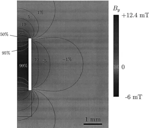
1 mm
Figure 2-7: Two dimensional simulation of magnetic field in cylindrical coordinates
y - . A 20 turn coil is modeled with 1 A current flow. The field lines show the
direction of B, and the color represents the magnitude of the
y
directed field.20 MHz
Figure 2-8: Two dimensional cylindrically symmetric about
cross section of current distribution. The images are the left side of the page. The coil has a larger resistance at high frequency because the current flows mostly on the inner surface of the coil.
2 MHz
0
0
0
Parameter Value Description
fo
20 MHz frequencyN 20 number of turns deoil 1.8 mm coil diameter rwire 40 pim wire radius
s 92 um turn spacing
I 1 A current
L 590 nH inductance
R 1.7Q a.c. resistance
Q
44 quality factorB I(0,0) 9 mT field at the center
Table 2.1: Simulation parameters and outputs for a 20-turn coil.
M
IL
1
L2 V2Figure 2-9: Mutual inductance represented in a circuit diagram.
2.3
Mutual Induction
Mutual inductance from a circuit perspective is the voltage induced in one conductor as a result of a changing current in a second conductor. The circuit diagram repre-sented has two inductors, L, and L2, with a mutual inductance between them, M,
to the voltages across them:
dii
Vi = L, di (2.12) dtdi
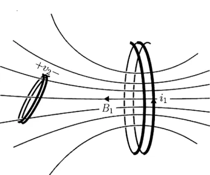
2 V2 = L2 di (2.13) dt dii V2 = M12 (2.14) dt di2 V = M21 dt. (2.15)Calculating the mutual inductance between two coils (see figure 2-10) requires knowl-edge of their geometry and relative orientation. Faraday's original experiments showed that a changing magnetic flux through a wire loop will induce a electromotive force around the loop. The changing magnetic flux is generated by the alternating current in a nearby coil[50]. Expressed mathematically the voltage in the loop is given by,
dt
S= dt , (2.16)
where 1 is the magnetic flux through the loop. If this flux is generated by current,
i, flowing in another conductor, then the mutual inductance is
M- -. (2.17)
The flux can be calculated by integrating the magnetic flux density, B, over the surface, S, bound by the loop
Figure 2-10: The field generated by a changing current in one coil induces a voltage,
v2(t) = -Mi, in a nearby coil.
where A is the normal to each differential surface element, dS[38]. This approach has two drawbacks. The field, B, is calculated using the Biot-Savart equation at each differential surface element. This is computationally expensive because the magnetic field would need to be calculated at many points in the three dimensional space bound by the second coil. The second drawback is that it is not obvious where there the surface, S, lies.
The magnetic vector potential offers a much faster and cleaner approach. Conven-tionally denoted by A, it is related to the magnetic flux density as follows,
V x A = B. (2.19)
integral of A, such that,
Ji -V x AdS= A -dl (2.20)
where 1 is the line bounding the surface S[51]. That line is the coil through which we want to calculate the flux. The vector potential from a line current, C, at a point
in space, , is given by,
A0p Idl
A(--)= , (2.21)
C
where r is the distance from the point ' to the point along C [38].
The mutual inductance between two coils can be calculated by integrating the vector potential A along the second coil C2. Combining Equations 2.17, 2.18, and 2.20 yields,
M = A -dl) (2.22)
C2
which combined with equation (2.21) gives,
/10 Idli
M
=
j
_. -d12 (2.23)C2 C1I
where r'j and r are points along C1 and C2. The circular integrals can be omitted knowing that C1 and C2 will be closed loops when connected in a circuit. Rearranging the terms yields a simplified form,
M= PO d1 d1 _ (2.24)