ASR dependent techniques for speaker recognition

ASR Dependent Techniques for Speaker

Recognition

by

Alex S. Park

B.Sc., Massachusetts Institute of Technology (2001)

Submitted to the Department of Electrical Engineering and Computer

Science

in partial fulfillment of the requirements for the degree of

Master of Engineering in Electrical Engineering and Computer Science

at the

MASSACHUSETTS INSTITUTE OF TECHNOLOGY

May 2002

@

Massachusetts Institute of Technology 2002. All rights reserved.

Author ..

. . . .

.

...

Department of Electic*1' En ineering and

Accepted by .

...

N

Chairman,

Committee

₅

RO F TECHR IGY

JUL 3 1 20

-ASR Dependent Techniques for Speaker Recognition

by

Alex S. Park

Submitted to the Department of Electrical Engineering and Computer Science on May 10, 2002, in partial fulfillment of the requirements for the degree of

Master of Engineering in Electrical Engineering and Computer Science

Abstract

This thesis is concerned with improving the performance of speaker recognition sys-tems in three areas: speaker modeling, verification score computation, and feature extraction in telephone quality speech.

We first seek to improve upon traditional modeling approaches for speaker recog-nition, which are based on Gaussian Mixture Models (GMMs) trained globally over all speech from a given speaker. We describe methods for performing speaker identifica-tion which utilize domain dependent automatic speech recogniidentifica-tion (ASR) to provide a phonetic segmentation of the test utterance. When evaluated on YOHO, a stan-dard speaker recognition corpus, several of these approaches were able outperform all previously published results for the closed-set speaker identification task. On a more difficult conversational speech task, we were able to use a combination of classifiers to reduce identification error rates on single test utterances. Over multiple utterances, the ASR dependent approaches performed significantly better than the ASR inde-pendent methods. Using an approach we call speaker adaptive modeling for speaker identification, we were able to reduce speaker identification error rates by 39% over

a baseline GMM approach when observing five test utterances per speaker.

In the area of score computation for speaker verification, we describe a novel method of combining multiple verification metrics, which is based on confidence scor-ing techniques for speech recognition. This approach was compared against a baseline which used logarithmic likelihood ratios between target and background scores.

Finally, we describe a set of experiments using TIMIT and NTIMIT which com-pare the speaker distinguishing capabilities of three different front end feature sets: mel-frequency cepstral coefficients (MFCC), formant locations, and fundamental fre-quency (Fo). Under matched training and testing conditions, the MFCC feature sets had perfect identification accuracy on TIMIT, but significantly worse performance on NTIMIT. By training and testing under mismatched conditions, we were able to determine the reliability of extraction for individual features on telephone quality speech. Of the alternative features used, we found that F0 had the highest speaker

distinguishability, and was also the most reliably extracted feature under mismatched conditions.

Thesis Supervisor: Timothy J. Hazen Title: Research Scientist

Acknowledgments

First, I would like to thank my thesis advisor, T.J. Hazen, who has been a patient and knowledgeable mentor throughout the course of this research. Over the last year and a half, his insightful comments and explanations have taught me a great deal about speech and research in general. I would also like to thank my academic advisor, Jim Glass, who has been an invaluable source of advice in matters large and small, from help in finding a research assistantship, to help in finding a dentist.

I am grateful to Victor Zue and the research staff of the Spoken Language Systems group for providing a supportive atmosphere for research and learning. I am also grateful to the students of SLS for many informative and entertaining discussions on

and off the topic of speech. Particular thanks go to Han and Jon for their help with many technical issues, and to Ed and Vlad for sharing many painfully fun nights of Tae Kwon Do practice.

I would also like to thank friends and family outside of SLS: Rob and Fred, for their perspectives on academic life; Nori and Jolie, for a fun year at the Biscuit factory; my uncle and his family, for providing a home away from home; my brothers, for always reminding me of our great times together in Canada; and especially Karyn, for always being a steady source of support and encouragement.

Finally, I am most grateful to my parents, whose unwavering love and support have been a source of motivation and inspiration throughout my life.

This research was supported by an industrial consortium supporting the MIT Oxygen Alliance.

Contents

1 Introduction 13

1.1 Background . . . . 13

1.2 Previous Work . . . . 15

1.3 Goals and Motivation . . . . 16

1.4 O verview . . . . 17

2 Corpora and System Components 19 2.1 Speaker Recognition Corpora . . . . 19

2.1.1 Y O H O . . . . 19

2.1.2 MERCURY, ... . 20

2.1.3 TIMIT & NTIMIT . . . . 20

2.2 The SUMMIT Speech Recognition System . . . . 22

2.2.1 Segment-based Recognition . . . . 22

2.2.2 Mathematical Framework . . . . 22

2.2.3 Finite State Transducers . . . . 23

2.3 Signal Processing Tools . . . . 24

3 Modeling Approaches for Identification 25 3.1 Gaussian Mixture Models . . . . 25

3.1.1 Background . . . . 25

3.1.2 Training . . . . 26

3.1.3 Identification . . . . 27

3.2 Alternative Modeling Approaches . . . . 27

3.2.1 Phonetically Structured GMMs . . . . 27

3.2.2 Phonetic Classing . . . . 28

3.2.3 Speaker Adaptive Scoring . . . . 31

3.3 Two Stage Scoring . . . . 31

4 Identification Experiments for Modeling 33 4.1 Experimental Conditions . . . . 33

4.1.1 Speech Recognition . . . . 33

4.1.2 Modeling Parameters . . . . 33

4.2 Comparison of Methods on Single Utterances . . . . 37

5 Confidence Scoring Techniques for Speaker Verification 5.1 Background ...

5.1.1 Rank-based verification . . . . . 5.1.2 Codebook based verification . . 5.1.3 Statistical verification . . . . . 5.2 Evaluation Metrics . . . . 5.3 Confidence Scoring Approach . . . . .

5.3.1 B-list Features for Verification 5.3.2 Linear Discriminant Analysis 5.4 Experimental Conditions . . . .

5.4.1 Corpus Creation . . . . 5.4.2 Training and Testing . . . . 5.5 R esults . . . .

6 Alternative Features for Speaker Recognition in Speech

6.1 Background .... ...

6.1.1 Mel-frequency Cepstral Coefficients . . . . 6.1.2 Formant Frequencies . . . . 6.1.3 Fundamental Frequency . . . . 6.2 Feature Set Experiments . . . ..

6.2.1 Feature Extraction Algorithms . . . . 6.2.2 Performance of MFCC Feature Set . .

6.2.3 Performance of Formant and Pitch Feature 7 Conclusion 7.1 Sum m ary . . . .. . . . . 7.2 Future W ork . . . .. . . . . Telephone Quality 63 . . . . 63 . . . . 63 . . . . 64 . . . . 66 . . . . 66 . . . . 66 Sets 67 67 73 73 75 . . . . 41 . . . . 41 . . . . 42 . . . . 42 . . . . 45 . . . . 49 . . . . 49 . . . . 50 . . . . 51 . . . . 51 . . . . 52 . . . . 53 41

List of Figures

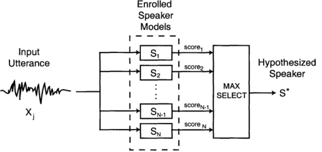
1-1 Block diagram of typical speaker identification system. The input ut-terance is scored against enrolled speaker models, and the highest

scor-ing speaker is chosen... . .. ... 14

1-2 Block diagram of typical speaker verification system. A verification score is computed from the input utterance and claimed identity. The verification decision is then made by comparing the score against a predetermined verification threshold. . . . . 14 3-1 Segment windows for computing frame level feature vectors. . . . . . 26 3-2 Finite-state transducer mapping input frame feature vectors to output

speaker labels . . . . 27 3-3 Phonetically Structured GMM scoring framework . . . . 29 3-4 Phonetic Class scoring framework . . . . 30 3-5 Two stage scoring framework allowing simultaneous speech recognition

and speaker identification . . . . 32 4-1 Finite state network illustrating constrained grammar for YOHO . . . 34 4-2 Combination of scores from multiple classifiers . . . . 37 4-3 Cumulative scoring over M utterances from a particular speaker . . . 39 4-4 Comparison of identification error rates over multiple utterances on

MERCURY corpus ... ... 40

5-1 Sample ROC curve for a speaker verification system. As the operating point moves to the right and the threshold is increased, the rate of detection approaches 1, as does the rate of false acceptance. As the operating point moves to the left, the false acceptance rate and the detection rate both go to 0. . . . . 46 5-2 Closeup of upper left hand corner of ROC curves on YOHO for

verifi-cation systems based on the four modeling methods from the previous

chapter. . ... ... . . . ... ... . 47

5-3 Equivalent DET curve to Figure 5-2 for verification results on YOHO. 48 5-4 Detection error tradeoff curve for baseline and Fisher LDA based

ver-ification m ethods . . . . 55 5-5 Detection error tradeoff curve for baseline and LDA based verification

5-6 Closeup of DET curve from Figure 5-5 showing low false alarm (LFA) region . . . . 57 5-7 Closeup of DET curve from Figure 5-5 showing equal error rate (EER)

region . . . . 58 5-8 Closeup of DET curve from Figure 5-5 showing low detection error

(LD E ) region . . . . 59 5-9 DET curve comparing performance of baseline system and LFA

opti-mized baseline system . . . . 61 6-1 Bank of filters illustrating the Mel frequency scale. . . . . 64 6-2 Representative spectra for transfer functions in Equation 6.1. . . . . . 65 6-3 Spectrogram comparison of identical speech segments taken from TIMIT

and NTIMIT. The NTIMIT utterance has added noise and is bandlim-ited to 4 kH z. . . . . 69 6-4 Identification accuracy of individual formants using GMM speaker

List of Tables

2-1 Example of a conversation with MERCURY . . . . . 21

2-2 Summary of corpus properties . . . . 22 3-1 Phone classes used for phonetically structured GMMs and phonetic

classing approaches. . . . . 28 4-1 Comparison of identification error rates for baseline approach with

dif-ferent numbers of mixtures on YOHO and MERCURY data sets . . . . 35

4-2 Comparison of identification error rates for Phonetically Structured approach when varying mixture counts and class weights . . . . 36 4-3 Comparison of identification error rates for each approach on YOHO

and MERCURY data sets . . . . 38

4-4 Identification error rates over 1, 3, and 5 utterances on MERCURY corpus 40

5-1 Summary of augmented MERCURY corpus properties. For the

aug-mented imposter sets, each speaker is present in only one of the two

sets. ... ... 52

5-2 Weighting coefficients of each verification feature for the baseline method

and three linear discriminant analysis results. The Fisher LDA vector

is the initialized projection vector used for the hill climbing methods. The three hill climbing LDA variations were optimized on low false

alarm rate (LFA), equal error rate (EER) and low detection error rate

(L D E ). . . . . 54 6-1 Identification accuracy of MFCC features on TIMIT and NTIMIT.

The first row indicates performance using models trained on TIMIT

data. The second row indicates performance using models trained on

NTIMIT data. The third row indicates expected performance of a random classifier. . . . . 67 6-2 Identification accuracy using feature vectors derived from formant sets

using GMM speaker models trained on TIMIT data . . . . 68 6-3 Identification accuracy and rank error metric of individual formants

using GMM speaker models trained on TIMIT data . . . . 70

6-4 Identification accuracy using FO derived feature vector using GMM

Chapter 1

Introduction

The focus of this work is to investigate and improve upon currently used techniques for modeling, scoring, and front-end signal processing in the field of automatic speaker recognition. Speaker recognition is the task of determining a person's identity by his/her voice. This task is also known as voice recognition, a term often confused with speech recognition. Despite this confusion, these two terms refer to complementary problems; while the goal of speech recognition is to determine what words are spoken irrespective of the speaker, the goal of voice recognition is to determine the speaker's identity irrespective of the words spoken.

In mainstream media and science fiction, automatic speaker recognition has beei depicted as being as simple as reducing a person's spoken utterance into a character-istic "voiceprint" which can later be used for identification. Despite this simplcharacter-istic portrayal, determining the unique underlying properties of an individual's voice has proven difficult, and a high-performance speaker recognition system has yet to be built.

1.1

Background

Speaker recognition is specified as one of two related tasks: identification and ver-ification. Speaker identification is the task of identifying a speaker from a set of previously enrolled speakers given an input speech utterance. Potential applications for speaker identification include meeting transcription and indexing, and voice mail summarization. A high level block diagram of a typical speaker identification system is illustrated in Figure 1-1.

A closely related task to speaker identification is speaker verification, which takes a purported identity as well as a speech utterance as inputs. Based on these inputs, the system can either accept the speaker as matching the reference identity, or reject the speaker as an imposter. Speaker verification is one of many biometric devices that are being explored for use in security applications. A high level block diagram

of a typical speaker verification system is shown in Figure 1-2.

An additional task distinction is the notion of text dependence. Text dependent systems assume prior knowledge of the linguistic content of the input utterance. This

Enrolled Speaker Models II sCore2 S2 SN-1 scoreN score _N FSN MAX SELECT Hypothesized Speaker S*

Figure 1-1: Block diagram of typical speaker identification system. The input ut-terance is scored against enrolled speaker models, and the highest scoring speaker is chosen. Input Utterance ) Score Computation "Accept" x ~score o S N "Reject" L - - -. -. ,

Claimed Enrolled Verification Verification Identity Speaker Models Threshold Decision

Figure 1-2: Block diagram of typical speaker verification system. A verification score is computed from the input utterance and claimed identity. The verification decision is then made by comparing the score against a predetermined verification threshold.

Input Utterance

knowledge is usually obtained by constraining the utterance to a fixed phrase (e.g. digit string). Text independent systems, on the other hand, assume no knowledge of what the speaker is saying, and typically exhibit poorer performance when compared to their text dependent counterparts. In spite of this, text independent systems are considered more useful, as they are more flexible and less dependent on user cooperation.

1.2

Previous Work

There are two main sources of variation among speakers: idiolectal, or high-level, characteristics, and physiological, or low-level, characteristics. Physiological vari-ations arise due to factors such as differences in vocal tract length and shape, and intrinsic differences in glottal movement during speech production. Although humans use these acoustic level cues to some extent when performing speaker recognition, they primarily rely on higher-level cues such as intonation, speaking rate, accent, dialect, and word usage [6]. Doddington [7] and Andrews [1] have recently demonstrated that idiolectal and stylistic differences between speakers can be useful for performing speaker recognition in conversational speech. However, since the usefulness of speech as a biometrically reliable measure is predicated on the difficulty of voluntarily chang-ing factors of speech production, research has generally focused on approaches that are based on low-level acoustic features.

Recent research in the field of speaker recognition can be roughly classified into three areas:

* Feature selection. What is an optimal front-end feature set which provides the greatest separability between speakers? In particular, what feature set remains undistorted and easy to extract in a noisy channel or in otherwise adverse conditions?

o Modeling. How should feature vectors from a particular speaker be used to accurately train a general model for that speaker? This is a difficult issue for text-independent tasks.

o Scoring and Classification. In performing speaker verification, what is an ap-propriate way of using scores generated by speaker models to reliably determine whether a speaker "closely" matches his/her purported identity?

With a few notable exceptions [17, 201, research in the field of feature extraction and front end processing has been relatively limited. Instead, most current systems use mel-scale cepstral features (MFCCs), and much of the recent research in speaker recognition has focused on modeling and scoring issues.

The use of Gaussian Mixture Models (GMMs) for text-independent speaker mod-eling was first proposed by Reynolds [24], and has since become one of the most widely used and studied techniques for text-independent speaker recognition. This approach models each speaker using a weighted sum of Gaussian density functions which are trained globally on cepstral feature vectors extracted from all speech for

that speaker. Recent variations of this method have included the use of phonetically structured GMMs [10], and the so-called "multi-grained" GMM approach investigated by Chaudhari et al. [4]. These techniques are described more fully in Chapter 3.

An alternative approach to global speaker modeling is the use of class-based speaker models. The benefit of using multiple models for each speaker is that the acoustic variability of different phonetic events can be modeled separately. However, this framework also requires a reliable method of assigning features from the test utterance into classes. In [25], for example, Sarma used a segment based speech rec-ognizer to model speakers using broad phonetic manner classes. Similar work was also done by Petrovska-Delacretaz in [21]. In this work, the use of unsupervised speaker class models was also studied, but results indicated that class-based models overall had worse performance compared to global models due to insufficient training data per class.

For speaker verification, a major obstacle is the determination of a suitable met-ric for gauging the closeness of claimant speakers to the target speaker. The pre-vailing approach for most systems is to score the input utterance against both the target speaker model and a universal background model which is a combination of all speaker models. The logarithmic likelihood ratio of these two scores is then used as a verification score which is compared against a pre-determined threshold. An alterna-tive approach to this problem has been presented by Thyes et al. [28], who used the concept of "eigenvoices" for verification. In that work, principal components analy-sis was used on feature vectors from a large set of training speakers to determine a subspace of feature dimensions, or "eigenspace", which captured the most variability between the speakers in the training data. Claimant utterances were projected into the eigenspace and were verified or rejected based on their distance from the target speaker vector, or "eigenvoice". The eigenvoices approach has been shown to perform well in cases where there is a large amount of data to train the eigenspace, and has

the benefit that performance is good even for sparse enrollment data.

1.3

Goals and Motivation

Although the goal of text independent speaker recognition has led to an increased fo-cus on global speaker modeling, it is well known that some phones have better speaker distinguishing capabilities than others [9]. Global speaker modeling techniques like the GMM approach are not able to take optimal advantage of the acoustic differences of diverse phonetic events. Conversely, phone level speaker modeling techniques ex-hibit poor performance due to insufficient training data at the phone level [21]. This work strives to address both of these modeling issues by using automatic speech recognition together with techniques borrowed from speaker adaptation.

A secondary goal of this thesis is to apply a new method of score combination to the task of speaker verification. While many systems attempt to find a single optimal verification metric, a fusion of metrics can potentially give better performance. We explore possible benefits of this approach using confidence scoring techniques.

for noise robustness issues. To this end, we explore the relative speaker distinguishing capabilities of formant locations and fundamental frequency measures in mismatched noise conditions.

1.4

Overview

The rest of the thesis is organized in the following manner. Chapter 2 describes the system, signal processing tools, and corpora used for this work. A detailed descrip-tion of baseline and ASR dependent approaches for speaker modeling is provided in Chapter 3, and performance and analyses of these systems on closed set speaker iden-tification tasks are presented in Chapter 4. Chapter 5 describes a novel framework for performing speaker verification using confidence scoring methods. Chapter 6 dis-cusses the speaker distinguishing capabilities of alternative features, such as formants and fundamental frequency. Finally, Chapter 7 closes with concluding remarks and provides some directions for future work.

Chapter 2

Corpora and System Components

2.1

Speaker Recognition Corpora

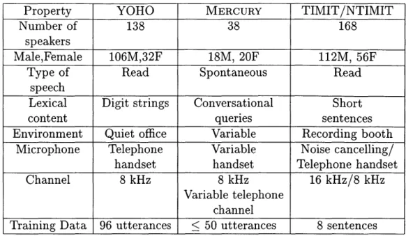
Over the course of this work, four corpora were used. The YOHO and MERCURY data sets were used to evaluate the performance of modeling approaches for speaker identification. An augmented version of MERCURY was also the primary corpus used for testing verification scoring methods. Finally, for evaluating the identification performance of different features, TIMIT and NTIMIT were used. The following sections give a description of the corpora, and the information is also summarized in Table 2-2.

2.1.1

YOHO

YOHO is a speaker recognition corpus distributed by the Linguistic Data Consor-tium [3]. As a standard evaluation corpus, many speaker recognition papers publish performance results on YOHO, making it useful for comparing the performance of different systems. The corpus consists of speech recorded from 106 male speakers and 32 females and attempts to simulate a verification scenario taking place in an office environment. Each utterance is a fixed-length combination-lock type phrase (e.g. "twenty-four, thirty-five, eighty-two"). During enrollment, each speaker was prompted with the same set of 96 digit phrases divided into four sessions of 24 ut-terances each. For verification, each speaker had ten sessions of four utut-terances each. Unlike enrollment, the verification utterances were not constrained to be the same across all speakers. The speech was recorded at a sampling rate of 8 kHz using a high-quality telephone handset, but was not actually passed through a telephone channel.

2.1.2 MERCURY

The MERCURY corpus is a speaker-labelled subset of data collected from the

MER-CURY air travel information system [26]. MERMER-CURY differs from YOHO in a number of ways. The type of speech is spontaneous, rather than read, and the 2300 word vo-cabulary includes city names, dates, and function words in addition to digits. Because MERCURY is a telephone-based system, the data in the corpus also has additional ad-verse conditions such as variable handsets and telephone channels, variable length utterances and out of vocabulary words. An example of a MERCURY user interaction is shown in Table 2-1.

For the closed set identification task, a set of 38 speakers was used. The training and test sets consisted of approximately 50 and 100 utterances per speaker, respec-tively. In addition, a development set was created from remaining data left over after training and test sets had been formed. The development set contained between 15 and 200 utterances per speaker.

For the verification task, an additional set of utterances taken from 80 imposter speakers was also created. The test set and development set were then augmented with these utterances by placing data from half of the new speakers in the test set, and the rest in the development set.

2.1.3

TIMIT & NTIMIT

TIMIT is a continuous speech corpus developed as a joint effort between the Mas-sachusetts Institute of Technology, Stanford Research Institute, and Texas Instru-ments. The speech data in TIMIT was recorded using a high quality microphone in a quiet recording booth. Although the full corpus consists of sentences read by 630 different speakers, the evaluations performed in this thesis used only a 168 speaker subset of the corpus. Each speaker read a set of ten sentences: two standard (SA) sen-tences, five phonemically rich (SI) sensen-tences, and three unique (SX) sentences. The SA sentences were the same across all speakers, and the SX sentences were unique to each speaker. The SI sentences were drawn from a pool of constructed phrases, and were therefore neither the same across all speakers nor unique to any particular speaker. For the speaker identification task, training was done on each speaker's eight non-SA utterances, and evaluation was performed using the two SA utterances.

NTIMIT is a speech corpus derived from TIMIT, and was developed in order to examine telephone channel effects on speech recognition performance for high quality data. NTIMIT data was obtained by playing TIMIT recordings out of a speaker into a telephone handset. The data was then passed through a land-line telephone channel and recorded. The training and test set partitioning was identical to that for TIMIT.

Mercury: Welcome to MERCURY, the MIT air travel planning system. I can help plan your air travel itinerary. Please tell me your user name. If you do not have a

user name, please say new user. User: New user.

MERCURY: Welcome. You have successfully logged onto MERCURY as a new user.

How may I help you?

User: I would like to fly from Boston to London

MERCURY: Flights from Boston to London. What date will you be travelling? User: Next Friday in the evening

MERCURY: Okay. flights from Boston to London departing between 5:00 pm and

midnight on June 25.. Can you provide a departure or arrival time? The earliest nonstop flight from Boston to London departing between 5:00 pm and midnight on June 25 leaves at 5:30 p.m. and arrives at 4:55 a.m. on British Airways. You

arrive one day later.

User: Is there a United flight?

MERCURY: Okay. United flights from Boston to London departing between 5:00

pm and midnight on June 25. One moment please... I have a nonstop United flight

leaving at 6:40 p.m. and arriving at 6:25 a.m.? User: Book that flight

MERCURY: United flight 998 has been added to your itinerary. You depart Boston at 6:40 pm and arrive in London Heathrow at 6:25 am. You arrive one day later. Shall I price your itinerary?

User: Yes.

MERCURY: The price for your itinerary is $2065.40. Is there anything else I can do for you?

User: No thank you. Good bye.

MERCURY: Thanks for using MERCURY. Have a nice day!

Property YOHO MERCURY TIMIT/NTIMIT

Number of 138 38 168

speakers

Male,Female 106M,32F 18M, 20F 112M, 56F

Type of Read Spontaneous Read

speech

Lexical Digit strings Conversational Short

content queries sentences

Environment Quiet office Variable Recording booth

Microphone Telephone Variable Noise cancelling/

handset handset Telephone handset

Channel 8 kHz 8 kHz 16 kHz/8 kHz

Variable telephone channel

Training Data 96 utterances < 50 utterances 8 sentences

Table 2-2: Summary of corpus properties

2.2

The SUMMIT Speech Recognition System

In this section, we give a brief overview of the components of the SUMMIT speech

recog-nition system. The speaker recogrecog-nition system built for this thesis used the existing

infrastructure of SUMMIT. In addition, the ASR dependent modeling approaches

described in the following chapter used word and phone hypotheses generated by SUMMIT. For a more detailed description of the system, see [13].

2.2.1

Segment-based Recognition

Unlike many modern frame-based speech recognition systems, SUMMIT uses variable-length segments as the underlying temporal units for an input waveforms.

Frame-based recognizers compute feature vectors (e.g., MFCC's) at regularly spaced time

intervals (frames), and then use those frame-level feature vectors to model acoustic events. Although SUMMIT initially computes features at regular time intervals, it then

hypothesizes acoustic landmarks at instants where large acoustic differences in the

frame-level feature vectors indicate that a boundary or transition may occur. These

landmarks then specify a network of possible segmentations for the utterance, each

one associated with a different feature vector sequence.

2.2.2

Mathematical Framework

In performing continuous speech recognition, the ultimate goal of any system is to

determine the most likely word sequence, i* = {w1, w2,. .. , WM}, which may have

be expressed as

* = arg max P (jA), (2.1)

With a segment-based recognizer, there are multiple segmentation hypotheses, s, each one associated with a different sequence of acoustic feature vectors, A,. Additionally, most words or word sequences, W', have multiple realizations as sequences of subword units, U'. To reduce computation, SUMMIT implicitly assumes that there exists an op-timal segmentation, s*, and subword unit sequence, i* , for any given word sequence. Equation 2.1 therefore becomes

{W*, i*, s*} = argrmaxP(, U, s, JA) (2.2)

Applying Bayes' rule, Equation 2.2 becomes

{*, i*, s*} = arg rnaxP(Ajz, i, s)P(slI, W)P(UIW)P(W) (2.3) In Equation 2.3, the estimation of the right-hand components is partitioned as follows

" P(A ,

'd,

P(A|J, i, s) = ] ₁ P(d Ili), where l4 is the ith landmark. If li occurs within a segment, then P(dilli) = P(dijui), and if li occurs at a boundary between two

segments, then P(dilli) = P('Iluiuii).

" P(s|'i, U') -Duration model. This component represents the likelihood of observ-ing a particular segmentation given a particular word and subword sequence. In the implementation of SUMMIT used in this work, duration models are not incorporated, so this value is constant.

" P(U'jw) - Lexical/Pronunciation model. This component represents the like-lihood of a particular subword sequence for a given word sequence. SUMMIT uses a base set of pronunciations for each word in the vocabulary [31]. Phono-logical rules are then applied to these baseforms in order to generate alternate pronunciations that account for common phenomena observed in continuous speech [16].

" P() - Language model. This component represents the a priori probability of observing a particular word sequence. SUMMIT uses a smoothed n-gram language model which associates a probability with every n-word sequence. These probabilities are trained on a large corpus of domain-dependent sentences.

2.2.3

Finite State Transducers

In order to find the optimal word sequence for Equation 2.3, SUMMIT models the search space using a weighted finite-state transducer (FST), R, which is specified as

the composition of four smaller FSTs

R = (S o A) o (C o P o L o G) (2.4) where:

" (S o A) represents a segment graph which maps acoustic features to phonetic

boundary labels with some associated probability score;

" C represents a mapping from dependent boundary labels to context-independent phone labels;

* P is a transducer which applies phonological rules to map alternate phone

re-alizations to phoneme sequences;

" L represents the phonemic lexicon which maps phoneme sequences to words in the recognizer vocabulary; and

* G represents the language model which maps words to word sequences with an associated probability.

The composition of these four FSTs, therefore, takes acoustic feature vectors as input, and maps them to word sequences with some output probability. The best path search through R is performed using a forward Viterbi beam search [23], followed by a backward A* beam search [30]. The final result of the search is an N-best list of the most probable word sequences corresponding to the input waveform.

2.3

Signal Processing Tools

For the non-cepstral features examined in Chapter 6, such as fundamental frequency

(Fo) and formant locations, values were computed offline using tools from the

En-tropic Signal Processing System (ESPS). ESPS is a suite of speech signal processing tools available for UNIX. Measurements for FO and voicing decisions were obtained using the get-f0 command, and formant locations were obtained using the f ormant command. More detail about the actual algorithms used in each of these tools is given in Chapter 6.

Chapter 3

Modeling Approaches for

Identification

In this chapter, we describe various modeling approaches used for speaker recogni-tion. In particular, several modeling techniques are illustrated for the task of closed-set speaker identification. We distinguish here between traditional text independent approaches which we classify as ASR independent, and ASR dependent approaches which make use of automatic speech recognition during speaker identification. The first section discusses the general theory of Gaussian mixture models (GMM), upon which each the modeling techniques are based. We then describe two ASR indepen-dent approaches followed by two ASR depenindepen-dent approaches. The final section details a two stage implementation strategy which allows combination of multiple classifiers.

3.1

Gaussian Mixture Models

3.1.1

Background

The most widespread paradigm for statistical acoustic modeling in both speech recog-nition and speaker recogrecog-nition involves the use of class-conditional Gaussian mixture models. With this approach, the probability density function for a feature vector, Z, is a weighted sum, or mixture, of K class-conditional Gaussian distributions. For a given class, c, the probability of observing Z is given by

K

p('1c) = W tc,k/(Z; Pc,k, Ec,k) (.1)

k=1

For speech recognition, the class c is usually taken to be a lexical, phonetic, or sub-phonetic unit. For speaker recognition, each class is usually taken to represent a different speaker. In Equation 3.1, We,k, Ac,k, Ec,k are the mixture weight, mean, and covariance matrix, respectively, for the i-th component, which has a Gaussian

distribution given by

; e - (3.2)

V

Although E can, in principle, represent a full covariance matrix, in practice, most implementations use diagonal covariance matrices to reduce computation.

In order to determine the parameters for the class conditional densities, a semi-supervised training approach is used. Assignment of training vectors to classes is done with prior knowledge of the correct classes, but the training of the class models them-selves is performed in an unsupervised fashion. Given a set of training vectors which are known to be in the class, an initial set of means is estimated using the K-means clustering [23]. The mixture weights, means, and covariances are then iteratively trained using the well-known expectation-maximization (EM) algorithm [5].

3.1.2

Training

Our baseline system was based closely upon Reynolds' GMM approach [24]. The class conditional probability densities for the observed feature vectors was the same as in Equation 3.1, with each class, C, representing a different speaker, Si.

K

P ziSi) = sjW(5; lsjk, -si,k), K

<64

k=1

For training, enrollment data was separated into speech and non-speech using a time aligned forced transcription produced by SUMMIT. The feature vectors from

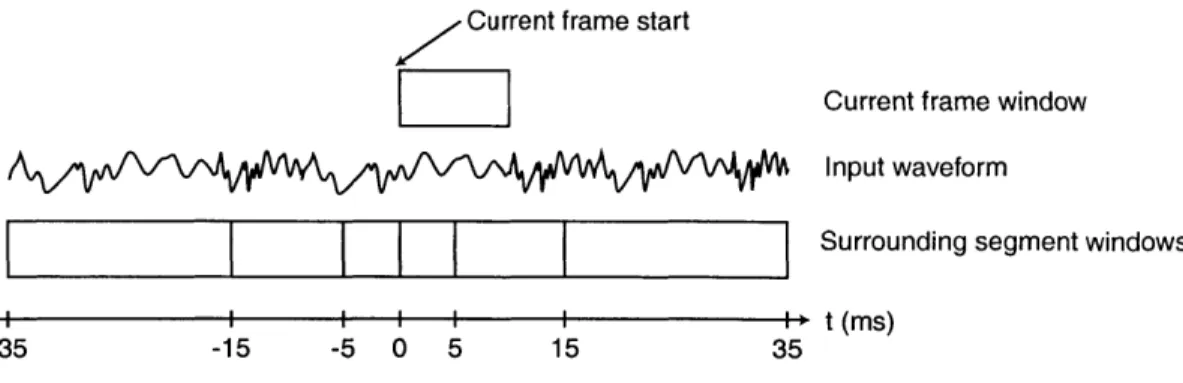
the speech segments, 5, were derived from 14-dimension mean normalized MFCC vectors. For each input waveform, 98-dimension vectors were created at 10 millisecond intervals by concatenating averages of MFCCs from six different segments surrounding the current frame. These additional segment level measurements, which are illustrated in Figure 3-1, were used to capture dynamic information surrounding the current frame. Principal components analysis was then used to reduce the dimensionality of these feature vectors to 50 dimensions [13].

Current frame start

Current frame window Input waveform

II

I I I

I

4

-35 -15 -5 0 5 15 35

3.1.3

Identification

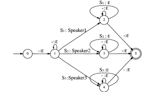
During recognition, we make use of a speaker FST, which constrains the possible state transitions for each input waveform, and also maps a sequence of input frame-level feature vectors to output speaker labels. An example speaker FST is illustrated in Figure 3-2. In Figure 3-2, the input labels "Si" and "-" refer to speaker and silence models, respectively. The input-output mapping in the speaker FST enforces the constraint that each utterance will only produce input feature vectors that are classified as either speech or non-speech (-), and that all speech samples from a single utterance will be produced by the same speaker. By using this FST together with speaker acoustic models in place of R in Equation 2.4, we are able to use SUMMIT to perform speaker identification by generating a speaker N-best list.

Si: E 2 Si: Speaker S2: -: -: E- :EF S2: Speaker2 -:F S3:s -: S3 :Speaker : 4

Figure 3-2: Finite-state transducer mapping input frame feature vectors to output speaker labels

3.2

Alternative Modeling Approaches

3.2.1

Phonetically Structured GMMs

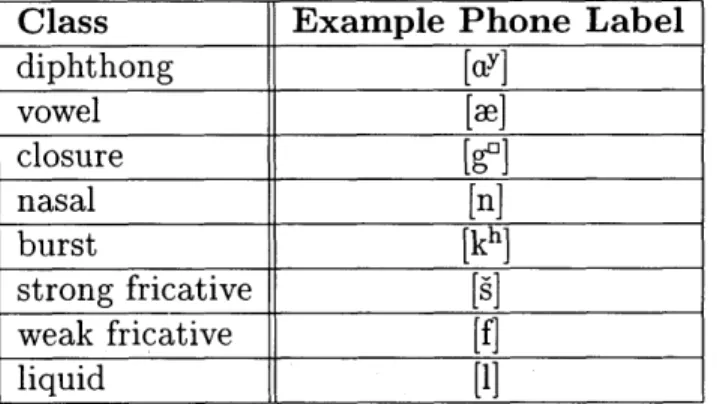
A recent variant of the traditional GMM approach is the so-called "phonetically-structured" GMM method which has been proposed by Faltlhauser, et al. [10]. During training, forced transcription of the enrollment data is used to separate frame-level features into broad phonetic manner classes. These classes are shown in Table 3-1. For each speaker, eight separate GMMs are then trained, one for each phonetic class. After training, these smaller GMMs are then combined into a single larger model using a globally determined weighting. We can contrast this approach with

the baseline by observing the structure of the speaker models

8 K

p(iFjS) = La [ wsi,k,cj/(; #SkC, Es2,kC,) (3.4)

j=1 k=1

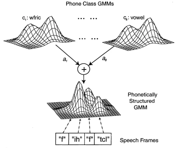
In Equation 3.4, Cj is the phone class, and aj and Kj are the weight and number of mixtures for Cj, respectively. The motivation for constructing the global speaker GMM in this fashion is that, this method is less sensitive to phonetic biases present in the enrollment data of individual speakers. During identification, all speech frames from the test utterance are scored against the combined model, as illustrated in Figure 3-3.

Class Example Phone Label

diphthong _[cLY] vowel

[m]

Table 3-1: Phone classes used for phonetically structured GMMs and phonetic classing approaches.

3.2.2

Phonetic Classing

The following two approaches, which we term ASR-dependent, require a speech recog-nition engine, such as SUMMIT, to generate a hypothesized phonetic segmentation of the test utterance. The generation of this hypothesis is described in Section 3.3.

The use of separate phonetic manner classes for speaker modeling was studied previously by Sarma [25]. This technique is similar to the use of phonetically struc-tured GMMs in that training is identical. Phonetic class GMMs are trained for each speaker, but instead of being combined into a single speaker model, the individual classes are retained. Each speaker is then represented by a set of class models, instead of a global model as in Equation 3.4.

p(iiSk, c1) =

Zni

p(ZS) = (3.5)

1p(

Phone Class GMMs

c,: wfric .... c.: vowel

Phonetically Structured

GMM

"f

"1ihi

f Iitc

Figure 3-3: Phonetically Structured GMM scoring framework

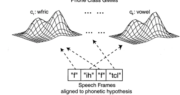
During identification, each test vector is assigned to a phonetic class using the phonetic segmentation hypothesis provided by the speech recognizer. The appropri-ate phone class model is then used to score the vector. This scoring procedure is illustrated in Figure 3-4.

Since test vectors are scored directly against the class-level GMMs, this approach is similar to the "multigrained" method proposed by Chaudhari et al. [4]. However, by using the phone class assignment provided by the speech recognizer, this approach eliminates the need to score against every model in the speaker's library, as is required by the multigrained method.

Phone Class GMMs

c: wfric

-44

f11

_"ih"

I

_{"f" "tcI"}

Speech Frames

aligned to phonetic hypothesis

Figure 3-4: Phonetic Class scoring framework

C8: Vowel

3.2.3

Speaker Adaptive Scoring

The previous two approaches attempt to improve upon the baseline GMM approach by using broad phonetic class models which are more refined than the global GMMs. At a further level of granularity, models can be built for specific phonetic events. Unfortunately, the enrollment data sets for each speaker in typical speaker ID tasks are usually not large enough to build robust speaker dependent phonetic-level models. To compensate for this problem, we can draw upon techniques used in the field of speaker adaptation. This allows us to build models that learn the characteristics of a phone for a given speaker when sufficient training data is available, and rely more on general speaker independent models in instances of sparse training data.

In this approach, speaker dependent segment-based speech recognizers are trained for each speaker. That is, rather than training class level speaker models, a separate

phone level speaker model is trained for each phonetic model in the speaker

indepen-dent speech recognizer. During iindepen-dentification, the hypothesized phonetic segmenta-tion produced by the speaker independent speech recognizer is used to generate the best path speaker dependent score, which is then interpolated with the recognizer's speaker independent score. This method approximates the MAP strategy for speaker adaptation [12]. Mathematically, if the word recognition hypothesis assigns each test vector Z to a phone

j,

p(ZSjS) = Ayp(Z|Mj,) + (1 - Aij)p(SzAMj) (3.6) where Mij, Mj are the speaker dependent and speaker independent models for phone

j,

n',j if _{n,3 >}

1;-'= 0 if ni, = 0, 1.

In Equation 3.7, nij is the number of training tokens of phone

j

r is an empirically determined tuning parameter that is the same across all speakers

and phones. For instances when ni, is equal to 0 or 1, the corresponding speaker dependent Gaussian, Mi,, cannot be trained, and the score is computed using only the speaker independent Gaussian.

3.3

Two Stage Scoring

In order to make use of speech recognition output during speaker identification, we utilize a two-stage method to calculate speaker scores. This framework is illustrated in Figure 3-5. In the first stage, the test utterance is passed in parallel through a speech recognition module and a GMM speaker ID module, which is implemented using the baseline approach. The speech recognition module produces a time-aligned phonetic hypothesis, while the GMM speaker ID module produces an N-best list of hypothesized speakers. These results are then passed to the next stage, where a second classifier rescores each speaker in the N-best list using one of the refined

techniques described above.

This two-stage scoring method is useful in a number of ways. First, by using the GMM speaker ID module for fast-match, we reduce post-recognition latency by limiting the search space of speakers presented to the second stage. Identification performance is not significantly affected since the probability of N-best exclusion of the target speaker by the GMM module can be made arbitrarily low by increasing N. Furthermore, there is little increase in pre-identification latency for the ASR depen-dent approaches since the GMM scoring proceeds in parallel with word recognition. Another advantage of this framework is that scores from multiple classifiers can be used and combined in the second stage.

Test uttera 1st stage 2nd stage[

nce

Figure 3-5: Two stage scoring framework allowing simultaneous speech recognition and speaker identification

Chapter 4

Identification Experiments for

Modeling

In this chapter, closed set speaker identification results are described for YOHO and MERCURY. We omit evaluation on TIMIT in this chapter because we were able to attain 100% identification accuracy on TIMIT using the baseline GMM approach. Instead, we reserve investigation of TIMIT and NTIMIT for Chapter 6, where we discuss benefits of different front-end features under adverse channel conditions.

4.1

Experimental Conditions

4.1.1

Speech Recognition

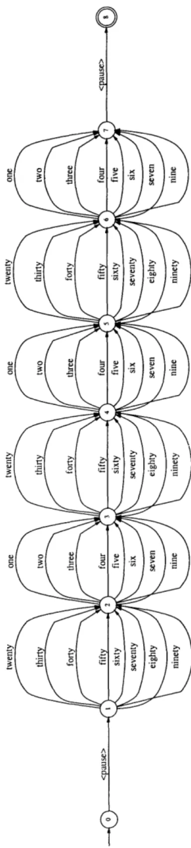
For both corpora we used domain dependent implementations of the MIT SUMMIT speech recognizer [13]. On the YOHO data set, the vocabulary and language model were limited to allow only the set of possible numerical combination lock phrases. Figure 4-1 illustrates the domain dependent finite-state acceptor (FSA) used to model the constrained vocabulary allowed in YOHO.

On the MERCURY data set, a recent version of SUMMIT currently deployed for

the MERCURY domain was used [26]. This recognizer was considerably more com-plex than the one used for YOHO, and included a 2300 word vocabulary suited for conversational queries regarding airline travel.

4.1.2

Modeling Parameters

For each of the modeling approaches that we used, performance was dependent on the choice of parameters specified in the Chapter 3. The relevant parameters for each approach were

* Baseline - Number of mixture components, K, from Equation 3.3.

" Phonetically Structured - Number of mixture components per class, Kj, and phone class weights, aj, from Equation 3.4.

A

U) 0 ~ 0

" Phonetic Classing - Number of mixture components per class, Kj, from

Equa-tion 3.5.

" Speaker Adaptive - Interpolation parameter, T, from Equation 3.7.

In addition to the model parameters for individual classifiers, weights for combining classifier scores must also be specified.

Determination of Mixture Numbers and Phone Class Weights

We first examined the effect of varying the total number of mixture components used in the global speaker modeling approaches. Initially, our choice of K = 64 for the baseline system was motivated by Reynolds' use of 64-mixture GMMs in [24]. We also used K = 64 x 8 = 512 in order to perform a fair comparison of this method against the Phonetically Structured approach with K, = 64. These results are shown in Table 4-1.

Error Rate _(%)

Method YOHO MERCURY

Baseline GMM (K=64) 0.83 22.43

Baseline GMM (K=512) 0.80 22.43

Table 4-1: Comparison of identification error rates for baseline approach with different numbers of mixtures on YOHO and MERCURY data sets

For the Phonetically Structured approach, we also performed similar experiments using Kj = 8, and K, = 64. These values corresponded to total mixture counts of

Ktot = 64 and Kit, = 512, respectively. In addition to varying the number of mixture components, we also used two methods for determining mixture weights

" Unweighted: a, = 1/(# of classes) " Weighted: a3 = Nj/Ntot

where Nj and Nt,, are the number of training tokens for phone class Cj and the total number of training tokens across all speakers, respectively.

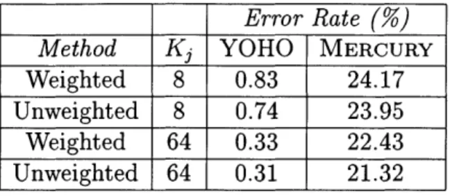
From the results in Table 4-1 and Table 4-2, we noted that weighting the phone class GMMs by their prior distributions in the training data resulted in worse per-formance than the unweighted GMMs. This was likely due to the fact that weight-ing with priors introduces bias against mixture components from underrepresented phone classes, which negated the main benefits of using the phonetically structured approach. The results also demonstrated that the phonetically structured models outperformed the baseline models when the total number of mixtures was large. The disadvantage of simply increasing K, is that the size of the global speaker model is increased, therefore requiring more computation to score each test utterance during identification.

Error Rate

_(%)

Method Kj YOHO MERCURY

Weighted 8 0.83 24.17

Unweighted 8 0.74 23.95

Weighted 64 0.33 22.43

Unweighted 64 0.31 21.32

Table 4-2: Comparison of identification error rates for Phonetically Structured ap-proach when varying mixture counts and class weights

For the phonetic classing approach, incorporation of automatic speech recognition reduces the need to "budget" the total number of mixtures among the individual phone class models. During identification, every frame of the test utterance is scored only against the phone class that it is assigned to. Therefore, computational complex-ity is a function of the number of mixtures per class rather than the total number of mixtures across all the class models for a particular speaker. For the phone classing approach, we set K = 64.

Determination of Interpolation Parameters for Speaker Adaptive Scoring For the speaker adaptive approach, we used linear interpolation to combine the speaker dependent and speaker independent scores at the phone level as described in Equations 3.6 and 3.7. In this approach, the interpolation factor for speaker i and phone j was specified by a global parameter, r, and the number of training tokens from speaker i for phone j, nij. In order to empirically determine an optimal value

for T, we performed identification experiments on the MERCURY development set.

We observed that identification accuracy generally improved as T was decreased from

100 down to 5. For values between 1 and 5, identification accuracy was not signifi-cantly affected. We used these results to set -r 5 for speaker adaptive scoring on MERCURY and YOHO.

In performing experiments to tune for r, an interesting result that we noted was that setting r = 0 yielded high identification error rates on the development set. As described in Section 3.2.3, this T value corresponded to using only speaker

depen-dent scores for phones with more than one training token, and speaker independepen-dent scores otherwise. This result confirmed our earlier suspicion that completely speaker dependent phone-level models would perform poorly due to an insufficient number of training examples for each phone.

Determination of Classifier Combination Weights

A primary benefit of the two-stage scoring framework described in Section 3.3 is the ability to combine scores from multiple classifiers, which can can often mitigate errors made by a single classifier. After an initial speaker N-best list is produced by the

Output from 1 st stageL

2nd stage

Combination

|"f" "ih" "f" 2.seker2

Classifier A Classifier B Refined Models

1. speaker, : XA,1 1. speaker₁: XB, 1

2. speaker2: XA,2 2. speaker₃: XB, 3 Rescored

3. speaker₃: XA,3 3. speaker_{2: XB,}

2 N-best lists

+

1.speaker,: aXA,1 a)XB,1

3. speaker₃: aXA,3+ (l-a)XB,3

2. speaker2: aXA,2+ (- a)XB,2 Combined N-best list

Figure 4-2: Combination of scores from multiple classifiers

GMM classifier in the first stage, a different classifier can be used in the second stage to produce a rescored N-best list using more refined speaker models. If the initial N-best list is passed to multiple classifiers, each one produces its own rescored N-best list. These rescored lists can then be combined and resorted to produce a final N-best list. This process is illustrated in Figure 4-2.

Although it is possible to use any number of classifiers, we only investigated pair-wise groupings using linear combination

Total score for Si = aXA,Si + (1 - a)xB,S (4.1)

In Equation 4.1, XA,SI and XB,SI are scores for speaker Si from classifiers A and B,

respectively. The combination weights were optimized by varying a between 0 and 1 on the MERCURY development set.

4.2

Comparison of Methods on Single Utterances

In order to investigate the advantages of each of the modeling approaches, we first computed results for the closed set identification task on individual utterances. These results are shown in Table 4-3. When comparing the performance of the different

classifiers, we observed that error rates on the YOHO corpus were uniformly low. In

particular, we noted that our best results on the YOHO corpus were better than the 0.36% identification error rate obtained by a system developed at Rutgers [3], which is the best reported result that we are aware of for this task. However, with the exception of systems involving the GMM baseline, each of the classifiers produced between 14 and 22 total errors out of 5520 test utterances, making the differences

between these approaches statistically insignificant.

On the MERCURY data set, the comparative performance of each system was more evident. Both the phonetically structured GMM system and the phonetic classing system had slight improvements over the baseline, while the speaker adaptive sys-tem has a higher error rate than any of the other approaches. Across all syssys-tems, we observed that error rates were significantly higher on the MERCURY task than on YOHO, clearly illustrating the increased difficulties associated with spontaneous speech, noise, and variable channel conditions. These factors also led to a higher word error rate for speech recognition on the MERCURY data, which partially explains why the recognition aided systems did not yield improvements over the baseline GMM method as observed with YOHO. However, we saw that by combining the outputs of multiple classifiers, lower overall error rates were achieved on both corpora.

Parameters _{Error Rate}

_(%)

Method K K. r o YOHO MERCURY

Baseline GMM 64 0.83 22.4

Phonetically Structured GMM (PS) 64 0.31 21.3

Phone Classing (PC) 64 0.40 21.6

Speaker Adaptive (SA) 5 0.31 27.8

Multiple Classifiers (GMM+SA) 64 5 0.45 0.53 19.0

Multiple Classifiers (PS+SA) 64 5 0.33 0.25 18.3

Multiple Classifiers (PC+SA) 64 5 0.30 0.25 18.5

Table 4-3: Comparison of identification MERCURY data sets

4.3

Comparison of Methods on Multiple

Utter-ances

Because of the non-uniformity of test utterance lengths on the MERCURY corpus, we performed additional experiments using multiple utterances for speaker identification on MERCURY. Multiple utterance trials were performed by combining the N-best list scores from single utterance trials for a particular speaker. For each M-wise grouping of N-best lists, each list was first normalized by the score of its lowest scoring speaker. The scores for each speaker were then added together over all M lists to create a cumulative N-best list which was then resorted. This method, which is illustrated in Figure 4-3, is equivalent to using cumulative speaker identification scores over several utterances.

Identification error rates over 1, 3, and 5 utterances are shown in Table 4-4. For all methods, scoring over multiple utterances resulted in significant reductions in error rates. We observed that the speaker adaptive approach attained the lowest error rates among the individual classifiers as the number of test utterances was increased (Figure 4-4). Moreover, as the number of utterances was increased past 3, the performance of the combined classifiers exhibited no significant gains over the speaker adaptive approach. When compared to the next best individual classifier, the speaker adaptive approach yielded relative error rate reductions of 28%, 39%, and 53% on 3, 5, and 10 utterances respectively.

Single Utterance N-best lists

Multiple Utterance N-best lists

1. speaker, : x, 1. speaker, : x, 1.speaker, :x, 1. speaker, : x1 2. speaker2: x2 2. speaker2: X2 2. speaker2: x2 2. speaker3: x3

3. speaker3: x3 3. speaker3: x3 3. speaker3: x3 3. speaker2: x2

Utt 1 Utt 2 Utt 1+M I Utt 2+M

~~~~- ---1. speaker,: _x, 1. speaker, : E x, 2. speaker_{3: x} 3 2. speakers : _{Z x} 3 3. speaker_{2: EX} 2 3. speaker2 _{: E x} 2 Utts: 1...(1+M) _{Utts: 2...(2+M)}