Avionics Systems Development for Small
Unmanned Aircraft
by
Vladislav Gavrilets
Submitted to the Department of Aeronautics and Astronautics
in partial fulfillment of the requirements for the degree of
Master of Science in Aeronautics and Astronautics
at the
R ,SSACHUSETTS INSTITUTE OF TECHNOLOGY
June 1998
@
Massachusetts Institute of Technology 1998. All rights reserved.
A uthor ... ...
...
Department of Aeronautics and Astronautics
May 22, 1998
Certified by ...
. ...
\
John J. Deyst
Professor of Aeronautics and Astronautics
Thesis Supervisor
Accepted by ...
S1
Jaime Peraire
Chairman, Department Committee on Graduate Students
JUL
Os)81"8
Avionics Systems Development for Small Unmanned
Aircraft
by
Vladislav Gavrilets
Submitted to the Department of Aeronautics and Astronautics on May 22, 1998, in partial fulfillment of the
requirements for the degree of
Master of Science in Aeronautics and Astronautics
Abstract
The avionics systems for two small unmanned aerial vehicles (UAVs) are considered from the point of view of hardware selection, navigation and control algorithm design, and software development. Some common challenges for many small UAV systems are addressed, including gust disturbance rejection at low speeds, control power, and systems integration. A rapid prototyping simulation framework which grew out of these efforts is described. A number of navigation, attitude determination and control algorithms are suggested for use in specific applications.
Thesis Supervisor: John J. Deyst
Acknowledgments
The work described in this thesis was a result of team effort. Here I would like to thank people who contributed to both projects described in the thesis, and otherwise provided support during my two years at MIT.
I would like to thank my advisor Professor John J. Deyst for giving me the op-portunity to work on an open-ended, challenging and rewarding project. Under his guidance I was able to get real world engineering experience.
Professor Mark Drela greatly contributed to the aerodynamic modeling and anal-ysis of the WASP flyer. Professor James Paduano helped with the analanal-ysis and design of the control augmentation system. I greatly appreciate Professor David L. Trumper's help with the vibration isolation problem. The value of the knowledge I acquired from all the above members of MIT faculty through classes and consultations is very hard to overestimate.
Draper Lab engineers Brent Appleby and John Plump provided simulation frame-work for the WASP project. Studying the experience of the DSAAV team, lead by Paul DeBitetto, provided an excellent source of empirical data and design guidelines. I would like to thank Tan Trinh, Torrey Radcliffe, Jean-Marc Hauss, Cory Hallam, Josh Bernstein and other students who worked on the WASP team in 1996-98.
My thanks to MIT Aerial Robotics team. Confidence and expertise of Scott Rasmussen and Jeremy Brown made this very complicated project a reality.
I would like to thank graduate students at the MIT IC&E lab. Stimulating dis-cussions with Jerry, Emilio, Eric and Arkadiy frequently helped me find a way to solve a problem.
Sergei, Jim and Akan were very supportive friends and roommates during my two years at MIT.
My special thanks to my family in Bishkek, Kyrgyzstan, for their caring letters, and sincere support in my endeavours.
Contents
1 Introduction
1.1 Background and Motivation . ... 1.1.1 Applications for Unmanned Aircraft
1.1.2 Avionics Challenges Specific to Small UAVs ... 1.2 Thesis Overview ...
2 Avionics Architecture for a Small Unmanned Helicopter
2.1 Aerial Robotics Competition . . . .. 2.2 Hardware Architecture ...
2.2.1 Driving Requirements . . . .
2.2.2 Overview of Subsystems . . . . 2.2.3 Selection Criteria for Navigation Sensors . . . . 2.3 Guidance, Navigation and Control Algorithms . . . .
2.3.1 Algorithm Reuse . . ...
2.3.2 Extended Kalman Filter Design for Navigation of Helicopter . ...
2.4 Software Architecture and Reuse . ...
3 Gun-Launched Surveillance Aircraft
3.1 Wide Area Surveillance Projectile . . . . 3.1.1 Project Background and Goals . . . ... 3.1.2 Overall Design ... 3.1.3 Testing Approach ... The 19 . . . . . . 19 ... . 20 . . . . . . 20 . . . . . . 21 . . . . . . 25 .. . . . 29 .. . . . 29 1998 39 39 39 40 41
3.2 Hardware Architecture for the Operational Vehicle 3.3 Hardware Architecture for the Flight Test Vehicle
3.3.1 Requirements and Constraints ... 3.3.2 Subsystems . ...
3.4 Software Design for the Prototype Vehicle . 3.4.1 Functionality . ...
3.4.2 Implementation Issues . ... 3.5 Model and Simulation Development ... 3.5.1 Approach to modeling . ...
3.5.2 Geometric and Inertial Properties of WASP 3.5.3 Equations of Motion . ...
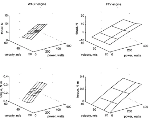
3.5.4 Aerodynamic Forces and Moments . 3.5.5 Engine Model . ...
3.5.6 Actuator Models ... 3.5.7 Sensor Models . ... 3.5.8 Gust Models . ...
3.5.9 Trim Analysis and Linearization ...
(FTV)
and FTV
3.5.10 Dynamics of Operational and Prototype Vehicle . 3.6 Control System Design . ...
3.6.1 Goals and Challenges . ...
3.6.2 Prototype Vehicle Command Augmentation System 3.7 Navigation and Attitude Determination Systems ...
3.7.1 Gravity Aiding with Strapdown Sensors ... 3.7.2 Velocity Matching . ...
3.7.3 Navigation System for Operational Vehicle ...
(CAS
4 Conclusion
A Nonlinear Model in Simulink
A.1 Block Hierarchy ... A.2 C-MEX vs M files ...
A.3 Animated Pilot-in-the-Loop Simulation . ...
A.4 Suggested Framework for Hardware-in-the-Loop Simulation ...
B Additional Data for Navigation Filter
B.1 Linear Propagation Matrix...
B.2 Measurement Matrices ... .
B.3 Conversion of Measurements to Center of Gravity B.3.1 Accelerometer Measurements . . . . B.3.2 GPS measurements ... B.3.3 Altitude measurements . . . . B.4 Field Heading ... 95 . . . . 95 . . . .. . 96 . . . . . 97 . . . . . 97 . . . . 98 . . . . . 98 . . . . 98
List of Figures
2-1 Robocopter on test field in Orlando, FLa . ... 20
2-2 Signal flow diagram for the 1997 helicopter . ... 24
2-3 Flow chart for onboard software ... .. 37
3-1 Deployed WASP flyer ... ... . 41
3-2 Signal flow for operational WASP . ... . . . . 44
3-3 Signal flow for prototype Vehicle . . ... .. . . 48
3-4 Software diagram for FTV ... ... 49
3-5 Engine thrust and roling torque for WASP and FTV. . ... 60
3-6 Shaping filter for gust inputs . ... .... 63
3-7 Open loop WASP and FTV longitudinal dynamics . ... 65
3-8 WASP and FTV open loop lateral dynamics . ... 66
3-9 Short period phasor diagram . ... .... 68
3-10 Phugoid phasor diagram ... ... 69
3-11 Root locus for inner pitch rate loop with lead, Kq = 0.06 ... 70
3-12 Root locus for nz/6e(s) transfer function with lag, Knz = 0.015 . . .. 72
3-13 Open loop, closed loop and loop transmission for q(s)/qcmd(S) transfer function ... . ... 72
3-14 Pitch rate pulse response with CAS-on . ... 73
3-15 Vertical gust response with CAS-on . ... 73
3-16 Pitch CA S . . . .. . 74
3-17 Dutch roll phasor diagram for the FTV . ... 75
3-19 Lateral SAS .. . . . .. . 76
3-20 Differential stabilizer pulse response . ... 77
3-21 Attitude determination system with gravity aiding . ... 79
3-22 Gravity aiding algorithm performance . ... 81
A-1 Simulation. Level 1: I/O ... 90
A-2 Simulation. Level 2: sensors and actuators . ... 90
A-3 Simulation. Level 3: equations of motion . ... 91
List of Tables
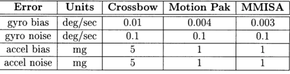
3.1 Power Requirements For Prototype Vehicle . ... 47 3.2 IMU Models ... ... ... 62 3.3 WASP and FTV Trim Conditions ... 64
Chapter 1
Introduction
1.1
Background and Motivation
1.1.1
Applications for Unmanned Aircraft
Unmanned aircraft are becoming increasingly important for both civilian and military applications. A number of situations exist in which human presence onboard the aircraft is either not necessary, too dangerous, or expensive.
Remotely piloted vehicles have been used for military purposes since the 1940s. Recent advances in sensors, communications, propulsion, flight dynamics and control algorithms have greatly increased the levels of autonomy that can be given to these vehicles. One can think of unmanned autonomous aircraft as a blend of two dreams of designers: the old dream of making flying machines, and the new dream of building smart robots.
The history of unmanned aircraft started with the Israeli Aircraft Industries decoy aircraft, used to confuse enemy anti-aircraft radars in 1972. A number of tactical surveillance aircraft from different countries followed. Currently, large long-endurance aircraft are being developed for reconnaissance, for atmospheric research and for aerial photography. There are a number of proposals for an unmanned tactical aircraft (UTA), which may replace manned combat aerial vehicles in the future.
the size of a hobby remote control (RC) aircraft and smaller. These include the micro UAV - a palm size surveillance aircraft that provides situation awareness for a soldier. Other applications include: traffic monitoring, search, and surveillance in the areas that are dangerous or difficult to access.
It is currently estimated [9] that there will be a $3.9 billion market for 7,900 UAVs in the next five years. The demand for unmanned aircraft will grow with the improvements in technology and, hence, reliability, of UAVs.
1.1.2
Avionics Challenges Specific to Small UAVs
There are a number of factors that are crucial for small unmanned aircraft. They can be loosely broken down into four categories: propulsion, light-weight structures, aerodynamic performance, and avionics system design and integration. The last of these includes sensors, communications, algorithms and software problems, which are considered here in application to two small UAVs.
Small aircraft fly at low Reynolds numbers, and thus it is difficult to achieve high lift to drag ratios. A number of efficient computational fluid dynamics (CFD) tools were developed that study flow behavior at this regime. Flying qualities of small aircraft are usually a serious issue due to lack of control power and vulnerability to gusts. The lack of control power arises mainly because of volume and weight constraints for control surfaces. Many designs need stability augmentation systems, and this requires high bandwidth sensor data. The flying qualities problem is coupled with the problem of avionics system design. Combining physical insights gained from new aerodynamic modeling techniques with modern control and estimation theory, can significantly aid in the design of adequate control systems using limited sensor data.
Experience has shown that the design and integration of avionics systems is one of the most complicated aspects of unmanned aircraft design. This is a problem with stringent constraints on size, weight and power consumption. The limited space available makes vibration from propulsion systems and electromagnetic interference adverse to sensor performance. Cost is a determining factor, because many small
vehicles are designed to be disposable. However, the choice of sensors, interfaces and software development practices can have a significant impact on cost. Proper use of rapid prototyping tools for software engineering and algorithm design can significantly reduce development time.
1.2
Thesis Overview
The objectives of this thesis are to summarize the development of avionics systems and some navigation and control algorithms used for two small UAVs, and to state lessons learned in the process. The field of small UAVs is very new, and the goal of this effort is to add to the common knowledge base in the area.
Specifically, Chapter 2 describes in detail the avionics system and navigation al-gorithms for a small unmanned helicopter. The helicopter was built as an entry in the International Aerial Robotics Competition by an MIT student team. The design of the system is based on designs made in previous years by MIT/Draper Laboratory teams, with certain changes aimed at improving performance. The thesis attempts to structure the process of hardware selection and system integration for a small UAV.
Chapter 3 describes an avionics system, model development, control and attitude determination algorithms, as well as a simulation framework for another small UAV. This vehicle is a gun launched aircraft, which is used to provide surveillance informa-tion using onboard sensors. This work has been done as a part of the MIT/Draper Technology Development Partnership Project.
Chapter
2
Avionics Architecture for a Small
Unmanned Helicopter
2.1
Aerial Robotics Competition
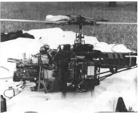
The small unmanned helicopter system, described in this chapter, was developed as the MIT entry in the 1997 International Aerial Robotics Competition. This contest dates back to 1991. The rules of the contest change from year to year, becoming ever more challenging. However the main goal is to develop autonomous aerial robots, capable of performing complex missions without human intervention. In 1997 the competition goal was to develop a fully autonomous VTOL aircraft, that could per-form search and removal of hazardous objects from a designated region. The vehicle had to take off and land autonomously, find the locations of black barrels marked with "radioactive" and "biohazardous" signs, and find and retrieve a small orange metal disc. The 1997 MIT team took second place in the contest with the helicopter based platform, shown in Figure 2-1.
The team demonstrated a fully integrated hardware system, communication, teleme-try and navigation capability. The 1997 design was based on the winning design of the Draper Laboratory/MIT team of 1996. The lessons from the 1997 effort are being used in ongoing design of the 1998 MIT entry.
Figure 2-1: Robocopter on test field in Orlando, FLa
2.2
Hardware Architecture
2.2.1
Driving Requirements
The choice of hardware for an aircraft is determined by its mission requirements. These are derived from high-level goal(s), which in this case is to score the highest number of points in the competition. The important derived requirements are:
* an image detection and recognition system for specified targets
* navigation accuracy of 0.3 m Spherical Error Probable (SEP)
* attitude and heading accuracy of less than 3 degrees * stable hover and forward flight
* autonomous takeoff and landing
e telemetry and monitoring system
* redundant safety system
2.2.2
Overview of Subsystems
Aerial Vehicle
The aerial platform chosen for the system was a Japanese TSK Blackstar helicopter. The TSK is a small 15 lb empty weight, 9 lb payolad, hobby helicopter, powered by a 2-cycle internal combustion engine. The payload capability of TSK was found to be marginal for the mission, and in 1998 a larger helicopter from the Bergen Machine Tool company was chosen.
Navigation Sensors
The navigation sensors included an inertial measurement unit, differential GPS, mag-netic flux compass and sonar altimeter. The design of the sensor subsystem is covered in detail in the next section.
Vision System
The onboard vision system consisted of the Cognachrome vision board connected to an RGB (red-green-blue) CCD camera. The board had custom software that was trained to recognize specific colors. Since disc retrieval was a major contributor in the scoring system, the vision system was designed specifically for finding and tracking orange color.
Power System
The power system used high efficiency switching regulators. Rechargeable NiCd bat-teries were used to supply electrical power.
Remote Control and Safety System
Safety of the system, for the contestants and spectators, was assured by an auto-matic/manual switch, that would allow a remote pilot to take over the computer con-trol in case of emergency. This switch was also used for test flights in manual mode when the navigation and telemetry systems were being tested. The auto/manual switch is one of the functions of the remote control receiver interface. The interface is a custom designed hardware element, developed by Draper Laboratory. It is based on a field programmable gate array (FPGA), and is wired to a Pulse Position Mod-ulation (PPM) receiver. The interface provides two other important functions. It writes pilot inputs to the onboard computer via a standard RS-232C serial proto-col, and reads control system commands from the computer, and converts them to servo commands. An important feature of the interface is its ability to operate in a pass-through mode, in which pilot commands are passed through the computer to the servos. This allows tuning independent control loops separately. In this case the pilot controls some channels, and computer controls the others. A separate RC receiver with its own battery is used to choke the engine in emergency situations.
Onboard Processing
The onboard computing power is provided by a 486DX2 50 MHz CPU with 8 Mb RAM and two RS-232C serial ports. The CPU is part of a PC104 stack with an ISA bus. The PC-104 is a standard format for hardware cards, ranging from CPUs to power supplies to low-cost GPS receivers. The cards are 90x96x26 mm, and can be attached to either a common PC-104 bus or the ISA bus. Other cards in the stack included a card with 4 RS-232C serial ports and an Ethernet card with the so called boot ROM. The latter is used to boot the CPU from a ground computer and upload the operating system (OS) and onboard executable code. The use of a hard drive for OS storage and data gathering on a small helicopter is unreliable because the vibration level is very high.
easier to use if PC104 videocard was used. This would allow the use of a monitor with the CPU to get a direct access to the onboard program without using a ground station display. Another improvement would be to use a PC104 standard power supply, which provides internal regulation for all cards in the stack. This prevents occasional CPU rebooting during spikes in the onboard power lines.
Communications Link
A two way communication link is provided by Proxim Proxlink radio modems, oper-ating in the 900 Mhz frequency range. The modems have a range of several hundred feet. They have a serial interface with internal checking for lost packets of data. The modems are used for uploading differential GPS corrections, for uplink of guidance commands and operator requests, and for downlink of telemetry information.
Ground Station
The ground station consists of a base GPS receiver, Pentium 100 MHz laptop with 8
Mb RAM and a radio modem.
Signal Flow Diagram
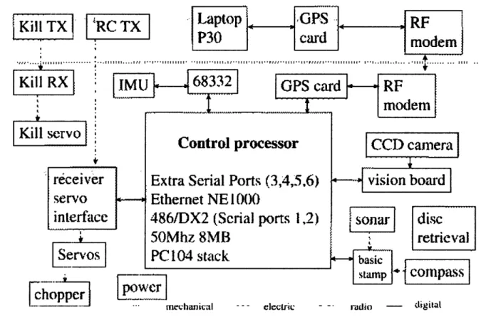
The signal flow diagram is given in Fig 2-2. The important feature of the architecture is use of only serial interfaces by the CPU. Each sensor requiring a more complicated interface, is sampled by a lower level processor. The IMU is sampled by a fixed point Motorola 68332 processor. The sensor interface was non-serial digital, and required an external clock rate signal at 1 MHz, which would be impossible to provide with the CPU. Basic Stamp was used to sample sonar altimeter and magnetic compass. Basic stamp is a chip which can be programmed with a simple set of commands in the Basic programming language. This architecture can be called distributed. It has an advantage with respect to a centralized architecture, that uses the CPU to sample sensors directly, because the CPU computing power is not required to perform input sampling.
Kill TXI
RC TX
L iLL Z~J ~'YI
receiver
servo
L
interface
Servos
chopper
68332
..LL._
power
. rn chanival --- electricGPS card -
RFe
CCD camera
-- vision board
Isonar
disc
."retrieval
asicsstamp
* compass
S rado -- igitalFigure 2-2: Signal flow diagram for the 1997 helicopter
Control processor
Extra Serial Ports (3,4,5,6)
Ethernet NE 10()
486/DX2 (Serial ports 1,2)
50Mhz 8MB
PC 104 stack
.. ...•i . ... . .!. . . .. . . .. . . . .Kill RX
• IMU
Kill Srv IIKill .v
Both ground based and onboard GPS receivers have two serial ports, and uplink and downlink commands are passed through from one port to another to insure the line
laptop <- >GPS <->modem <- >modem <- >GPS < - >CPU
2.2.3
Selection Criteria for Navigation Sensors
The designer of an avionics system must go through a set of trade offs in the selection process. The main considerations, common for all sensors are:
* performance requirements * power requirements * weight
* size, shape and volume * cost
* ability to operate in the environment onboard an aerial vehicle * ease of interfacing
The performance requirements for the sensors are derived from the attitude deter-mination and navigation accuracy requirements. The designer must determine that all of the important variables, including sensor drifts or biases, are observable from the chosen set of measurements. The sensor set should have bandwidth at least a decade above the vehicle dynamics. The correctly tuned estimation algorithm adjusts its bandwidth to take information from each sensor at the frequency range where the sensor performance is the best. The preliminary requirements on accuracy of sensors are derived from measurement equations. For example a 5 mg accelerometer bias, when used to correct low frequency gyro drifts, will result in a low frequency error in estimation of local vertical of .005(180/7r) a 0.3 degrees. In more complicated cases,
the design of the estimation algorithm has to be performed and covariance simulation run to determine the impact of errors. In the case considered in this chapter, the set of navigation sensors consisted of the inertial measurement unit, GPS receiver with base station for differential corrections, a sonar altimeter, and a magnetic flux compass.
Inertial Measurement Unit (IMU)
The strapdown IMU provides high-bandwidth measurements of the vehicle inertial angular rate and acceleration resolved into body axes. These measurements are used for the inner loops of the control system, and for the time propagation of the naviga-tion equanaviga-tions. The IMU is the heart of naviganaviga-tion system, and care must be taken in making its selection. A detailed study of IMU use in unmanned helicopters is given in [35]. Designs without an IMU were used in the past by Stanford University teams, which relied on multiple antenna high update rate GPS receivers for attitude information. The advantages of using an inertial measurement unit are a much higher bandwidth, higher reliability and integrity. Other sensors, such as GPS receiver can be used to compensate for IMU drifts, and to provide terrain information, in case of sonar altimeter. For application to small aircraft, with short mission times, the main performance characteristics of the IMU are bandwidth, short term bias stability, scale factor errors, and noise. The performance tables for several inertial measurement units are given in Table 3.2.
The noise level can be attenuated by choosing an A/D board with a larger number of quantization bits, shielding analog lines from EM interference, and mechanically isolating the sensor from high-frequency vibrations. A very important consideration is the full scales for both gyros and accelerometers. The full scales should not only be higher than the maximum accelerations and angular rates induced by vehicle dynam-ics, but also exceed the residual vibration level, not damped by the mechanical filters. The vibration level in a small aircraft can be as high as 10-100 g's, at frequencies as low as 20 Hz. The main sources are engine vibrations and rotor misalignment. The IMU should be put on flexures to reduce vibrations. An ingenious design of flexures
was suggested by Draper '96 team - the flexures were folded mousepads, which in effect creates a second order low-pass filter. The vibration sources, like an engine, should be isolated with anti-vibration mounts. In the example of vibration induced by engine piston, the mount can be rigid in directions perpendicular to piston motion, and very flexible in the direction parallel to it. If the residual vibration level does not saturate the sensors, analog filters with roll off frequencies above vehicle dynamics can be used. A higher sampling rate is beneficial to avoid aliasing of high frequency noise from vibrations into the relatively low frequency region of the rigid body dynamics.
GPS receiver
A GPS receiver provides excellent low frequency position and velocity information, especially in the horizontal plane. The receiver measures distances to the GPS satel-lites, and then finds its position in earth-fixed coordinates by triangulation, using accurate knowledge of satellite positions. Two sets of range measurements are used: the time interval the signal travelled from satellite to the receiver (called pseudor-ange), and the fractional number of the signal wavelengths (called carrier phase, or integrated Doppler). The second measurement is obtained by integrating the Doppler shift due to satellite motion, and contains the initial value of the integral (ambigu-ity), which has to be determined. This value is an integer, and algorithms exist for its resolution. The common error sources for GPS are the selective availability (SA), which is a pseudo random noise signal introduced by US government, multipath (a receiver mistakenly uses a reflected signal instead of the true signal), ionosphere and troposphere delays. Using correction signals from a second GPS receiver, placed at a known location, allows the elimination of SA and reduces the ionosphere and tropo-sphere delays, provided the receivers are located close to each other. This technique
is called differential GPS, or DGPS. Also, receivers that use two standard frequencies can correct for ionospheric delay, because it is frequency dependent. Choke rings should be used for ground station antennas to avoid multipath errors and geodesic tripods help as well.
integrity (i.e. the continuity of the signal tracking without dropouts or failures). Accuracy is provided by using DGPS, carrier phase measurements with integer am-biguity resolution, and dual frequency receivers. Integrity depends on the receiver technology used to keep track of satellites, and the number of satellites tracked by the receiver. GPS/GLONASS receivers, for example, can provide better integrity than GPS-only receivers because of the increased number of satellites available at any point in the world. The satellite lock can be poor due to both antenna vibra-tion and receiver vibravibra-tion. The latter affects the performance of the oscillator, that provides frequency reference for the receiver components. Loss of GPS track leads to significant performance degradation of navigation solutions, and the IMU should be good enough to keep the system operational until reacquisition. In the case of this unmanned helicopter, the safety pilot should have several seconds to notice that GPS track is lost and take over the control of the vehicle [19]. Longer reacquisition times directly result in tighter requirements on IMU performance. The sampling rate of a GPS receiver can be important if it is used without an IMU.
GPS technology leads to a significant reduction in the cost of avionics systems, because the IMU drift requirements become much less stringent in GPS/INS systems compared to a stand-alone INS. At the current state of technology, improvement in IMU performance is very costly compared to improvement in GPS performance.
Surveys of available GPS receivers are published annually in [33].
Sonar Altimeter
The sonar gives high bandwidth altitude information by sending acoustic signal pulses and measuring the signal return time. This information is used during landing. Se-lection criteria are accuracy and bandwidth.
Magnetic Compass
A compass provides low frequency heading information by measuring the direction to the local magnetic north. The criteria are accuracy and availability of tilt compen-sation.
Non-performance based criteria
Great care should be taken in selecting avionics sensors for small UAVs based on power requirements, size, and weight. The issue of power requirements for the IMU and CPU was not given proper attention in 1997, and this led to increased battery weight, a complicated power board design and extensive weight reduction of the vehicle structure. The power requirements should be kept to as few voltage levels as possible to avoid unnecessary power regulation. This is becoming increasingly feasible, since most electronics tend to use a few standard voltages (e.g. ±5, ±12 V). A detailed electronic system design for a small helicopter is given in [35].
Convenient sensor interfaces are vitally important. The time spent on develop-ment of device drivers and analog prefilter circuitry directly results in program costs. The simplest interface is a serial port. It is, at the same time, often inflexible because it restricts sampling rate and does not allow analog prefiltering. The sampling rate problem is likely to be mitigated with faster electronics. The sensor bandwidth and internal prefiltering can usually be specified by the customer. In addition to saving development time, another great advantage of a serial interfaces is its adaptability for hardware-in-the-loop simulation. Reproducing analog outputs from a digital sim-ulation can often be costly, in comparison to purchasing additional serial cards for the simulation computer. An integrated simulation framework is suggested in Ap-pendix A.
2.3
Guidance, Navigation and Control Algorithms
2.3.1
Algorithm Reuse
The 1997 and 1998 MIT teams used the same sensor configuration as MIT/Draper Laboratory DSAAV (Draper Small Autonomous Aerial Vehicle) used in 1996. In 1997, the performance of the sensors was close to that of 1996 sensors, and the MIT team completely reused the MIT/Draper '96 team algorithms for guidance, naviga-tion and control (GN&C). The control logic employed in the 1996 design used a set of
proportional, integral and derivative (PID) inner control loops, and waypoints were used for outer loop guidance. These algorithms were a result of 2 years of experiments with autonomous helicopters, and proved to be robust, flexible and tunable in flight. In 1997, the navigation algorithm, based on an extended Kalman filter (EKF), was tuned by changing the measurement and driving noise covariance matrices. Naviga-tion and control were run on board, and the guidance algorithm was run in a ground station computer. The description of GN&C algorithms used in MIT/Draper 1996 helicopter system is given in [19].
In 1998 the sensor performance has changed considerably: the IMU, GPS and compass were significantly different. The '98 Crossbow IMU had much larger biases than the '96 Motion Pak and '97 GEC Marconi units. On the other hand, a Novatel 2 receiver showed considerable improvement in performance with respect to RT-20 due to higher reliablility of in-flight ambiguity resolution. Also, a TCMVR-RT-20 magnetic flux compass from Precision Navigation gave better heading angle estimate and provided direct measurements of roll and pitch angles. Thus, the need to update '96 EKF has emerged and the detailed design of a new EKF for use in 1998 MIT helicopter is given in the next section.
2.3.2
Extended Kalman Filter Design for Navigation of The
1998 Helicopter
Selection of States
The navigation computations are performed using two reference frames: a local north-east-down (NED) frame, with the center of coordinate system chosen at the location of the GPS base station, and an aircraft body frame with its origin at the aircraft center of mass, X axis forward and Z axis down. The DSAAV navigation algorithm [19] used 11 states. Three more states, corresponding to gyro biases were added to account for poorer IMU performance. The resulting state vector is
where XL, YL, ZL are vehicle positions relative to the ground station in NED frame, UB, VB, WB are body axis velocity vector components; qo, q1, q2, q3 are a quaternion
representation of attitude, g is a gravity acceleration estimate, y1, 72, 73 are gyro bias states. Gravity acceleration state implicitly accounts for accelerometer biases and thus improves the attitude estimate [29]. The quaternion is a minimal representation of attitude which is free of singularities. However, there is a recurring need to normalize the quaternions after each time propagation or measurement update step:
q (2.2)
where= [qoq1 q2 q 3], and 1 12 =j -.q
Time Propagation Equations
Between measurement updates the state estimate is propagated using the nonlinear differential equation:
S= f ( , a) d, (2.3)
where Z are the rate gyro measurements and a are the accelerometer measurements. The inertial sensors are precalibrated before flight to account for biases. The inertial unit should be given a 20 to 40 minute warm up time to avoid transient temperature dependent bias and scale factor changes, at which point the calibration procedure could be started. Estimates of body rates and accelerations are formed from sensor outputs in flight:
WB = WIMU X SF w - Wbias
aB - aIMU X SFa - abias
where SF, and SFa are gyro and accelerometer biases. Accelerometer measurements must be transferred to c.g. location to correct for the IMU moment arm (Appendix B). Define the following vector arrays PL = [XL YL ZL, VB = [UB VB WB], q = [q0 q1 q2
q0 + q - q- q3 2 (qlq2 - qoq3) 2 (qlq3 + qoq2)
C 2 (q1q2 + qoq3) q2 - q2 + q2 - q3 2 (q2q3 + qoq1)
2 (qiq3 - qoq2) 2 (q2q3 - q0oq) q - q - q + q 2
Define 3D and 4D skew-symmetric matrices for 3D vectors:
Q4 = Then nonlin 0 -WY Wz We 0 Wz -Wy Wy -Wz 0 Wx Wz WY -Wx 0 1 4 = 0 -YX -YZ 7YX 0 7z -%y 0 -W z W 0 -- Y -3 = WZ 0 -wx F3 = YZ 0 -wy Wx 0 -/y 7x
ear propagation equations can be written as:
PL VB _C B = + C1g - (Q3 - F3 ) UB 2 (Q4 - r4) 2 (2.7) g= 0 7= 0
These equations can be numerically integrated at the IMU sampling rate using a first or second order integration routine. The IMU sampling rate of 25 Hz proved to be sufficient using a first order integration routine.
The nonlinear propagation equations can be linearized, with the Jacobian matrix
A (, x, , =)
19X (2.8)
This matrix is used to propagate the error covariance matrix between measurement (2.4) 7Yz 0 Yy -z 0 7x 0 (2.5) (2.6)
updates:
P = A(, )P + PAT(2, 0) + Q (2.9)
where Q is the process noise intensity matrix, which is used to model errors of inertial sensors. Typically the Q matrix is chosen to be diagonal. The suggested initial guess for main diagonal values is derived from sensor covariances:
Qd l[ 2 I 2 x4 2 1
]
(2.10)where Oa, a9 are the estimated accelerometer and gyro noise rms values, and cab,
agb are bias stability rms values, and 7 is the sampling rate of inertial sensors. The
scaling by 1/T is needed to account for the fact that the equations are integrated numerically with time step 7 [14]. The a parameters can be used to tune the system for maximum performance.
A first order integration of equations 2.9 proved to be satisfactory. The continu-ous propagation equations can be discretized, and a discrete version of propagation equations can be used [14]. The Jacobian matrix A is a sparse matrix, given in Appendix B.
Measurement equations
At the instances of time when the updates of DGPS, sonar altimeter or compass occur, the measurement update equations are used. Let h(x) be the nonlinear measurement function of state, and let
H Oh(x) (2.11)
Then the EKF measurement update equations are given by [14]
K = PHT [HPHT + R]
2+ = - + K [z - h(i)] (2.12)
where K is the filter gain, R is the measurement noise covariance matrix, and z is the measurement. In some instances the inversion of the symmetric matrix in equation 2.12 may become close to singular, so the computer may not have a sufficient number of bits (16 would be marginal) to assure positive eigenvalue. In this case the computations are unstable, so the square root implementation of the KF should be used [14].
DGPS is used to correct low-frequency drifts in position, velocity and attitude estimates. The sampling rate of the RT-2 receiver is 4 Hz. DGPS provides anntenna position and velocity information in the local NED frame. This data must be trans-ferred to the vehicle c.g. location (Appendix B). The linearized equations for GPS measurements are:
Hp=
[
3x3 03x3 03x4 03x1 03x3(2.13)
H=
[
O3x3 C Hvq 03x1 03x3]
(2.14)The block Hvq is given in Appendix B. Standard deviations of position and velocity measurement are provided as outputs from the GPS receiver. These estimates take into account the current state of the internal receiver KF, whether ambiguities are resolved, the number of satellites etc. These values are used to determine the measurement noise covariance. Under normal operating conditions, when the estimate has converged, the standard deviation of horizontal position measurement error is
up = 0.02 m, and horizontal velocity measurement error standard deviation is av =
0.003 m/s for RT-2 receiver. Vertical position and velocity error standard deviations maybe 3-4 times larger than horizontal. In the data sheets for RT-2 receiver the specified time to convergence after GPS acquisition is around 12 min if at least 6 satellites are available, thus the receiver should be started during the IMU warm-up.
DGPS provides altitude information relative to the location of the base receiver. To take into account terrain information during landing, the sonar altimeter is used. Sampling rate for the sonar is chosen to be 5 Hz. The altimeter measurement updates
are used only if the measured altitude is between 0.5 m and 6 m. The altimeter sends a pulse and shuts down so that it does not mistakenly take the emitted signal for the reflected one. This explains the lower limit on sonar measurements. Sonar measurements are also transferred to c.g. location (Appendix B). The standard deviaton of sonar measurement error increases with altitude, at low altitude it is orh
10 cm due to grass and other surface non-uniformity. The linearized measurement equation is:
Hh
[
0 0 1 01x3 01x4 Ox 01x3]
(2.15)For the case of a non-maneuvering vehicle, the heading angle is unobservable in the GPS velocity measurements (see Section 3.7.2). Magnetic compass updates are used to correct low-frequency drifts of the heading angle estimate. A sampling rate of 1 sec is sufficient. The TCMVR-20 compass also provides roll and pitch angle estimates. These are used inside the compass to correct heading information for tilt. However, if CPU time allows, these measurements can be used in the EKF as well. The compass measurement is corrected for magnetic variation, i.e. local direction to magnetic North with respect to true North. The accuracy for compass measurement is cr p 2 degrees. The linearized measurement equation for heading measurement is
He =
[
01x 01x3 Hq 01 01X3]
(2.16)where Hoq is given in Appendix B.
2.4
Software Architecture and Reuse
A major part of the onboard and ground station software from the 1996 system was reused. Both ground station and onboard software were implemented in the C programming language under the QNX operating system (OS). The QNX OS is a multitasking operating system, allowing several independent processes to be run simultaneously.
In retrospect, the decision to reuse the software was not justified. A summary of the major functions of the '97 software is presented and the reasons why it was hard to reuse the '96 software are given in the following paragraph. Ways to improve software design for an unmanned helicopter are suggested as well. Detailed descriptions of the '96 onboard and ground station software is given in [19].
The three major functions of the onboard software were navigation, control and communication. The ground station functions include mission planning, waypoint guidance, processing of vision information, communication, and the operator inter-face. The vision processing code takes information from the Cognachrome vision board, indicating the location of orange pixels in the camera field of view. It decides whether there is a disc, and estimates the disc coordinates based on the current state of the helicopter. The mission planner adds this location as a new entry into waypoint list. The guidance logic converts the waypoint list into low-level position, velocity and heading commands for the onboard control loops. Implementing the guidance logic in the ground station introduces a delay, and it is recommended that it be incorporated onboard the vehicle.
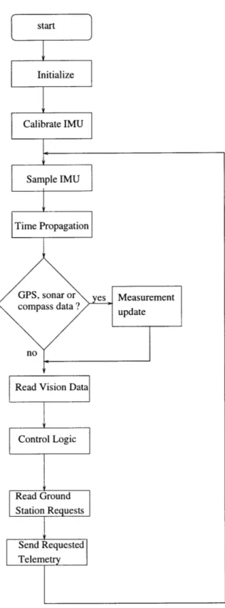
Figure 2-3 illustrates a high level flow chart for the onboard software. The onboard processor communicates with the external devices via serial ports, using non-blocking I/O. This means that the main program will not hang up in case the device being sampled fails. This is an important safety feature. However, it would be logical to use the multitasking capability of QNX OS to have separate processes for interfacing with devices, for control and navigation logic, and for communication. This would allow better timing for the processes, and easier debugging due to higher modularity. A good rule for software engineering is to keep different functions in separate files, otherwise the code becomes very hard to debug. With the exception of interfaces, all code that implemented the flow chart above was contained in a single file, which made this software difficult to reuse.
A simple example of the multitasking design approach to the onboard software for unmanned aircraft is given in Section 3.4.
Figure 2-3: Flow chart for onboard software
Chapter 3
Gun-Launched Surveillance
Aircraft
3.1
Wide Area Surveillance Projectile
3.1.1
Project Background and Goals
The avionics system development for an autonomous surveillance aircraft is pre-sented in this chapter. The effort described here was done under the sponsorship of Draper Laboratory as a part of the MIT/Draper Technology Development Part-nership Project. The major goal of the project was to develop entrepreneurship and innovation in engineering students. The primary requirement was to create an inno-vative product that would meet a major US national need.
During the fall term of 1996 a team of students, MIT faculty, and engineers from Draper Laboratory proposed several ideas, all related to aerospace. The group per-formed market assessments and preliminary technical evaluations of the concepts, and finally selected the Wide Area Surveillance Projectile (WASP) concept. WASP is a small gun launched aircraft, designed to meet a need for fast-response surveil-lance capability. A set of requirements for the vehicle was determined with potential customers (Navy, Army, Defence Airborne Reconnaissance Office) and the sponsor (Draper Laboratory). The requirements were further adjusted as the design
pro-gressed, and final estimates of the required performance are: * 15,000 g launch environment
* 15 min. loiter time * 15 km range
* 250 m radius of camera field-of-view, still frame or video image
* fit inside a 5" shell diameter
* 2-way datalink capability
* GPS-based waypoint guidance
In a typical scenario, WASP is launched from a 5" Navy gun, reaches its destination point (15 km range, and altitude of 500 m), is deployed from its shell, and starts sending still images or a videostream, and positioning information of designated points to a ground station. A ground operator designates new waypoints for the vehicle and commands its search pattern. Recognition of points of interest is performed by the operator, and positions of points of interest are determined using a combination of onboard navigation and camera pointing information.
3.1.2 Overall Design
This section provides a brief description of the overall vehicle design. A detailed discussion of the structural design, deployment mechanisms and aerodynamic design are given in [20] and [6].
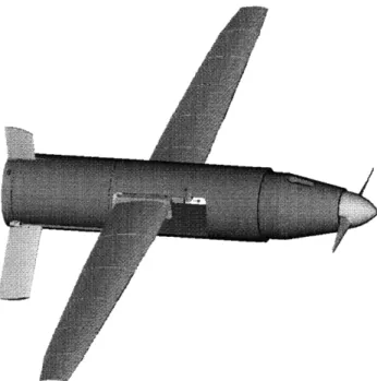
The flyer is stowed inside a 5" fin-stabilized artillery shell, derived from a re-designed illuminating round. At a predetermined time after gun launch an onboard timer triggers separation of the shell base, and a parachute is deployed. The parachute decelerates the vehicle to a sufficiently low dynamic pressure to allow deployment of the wings, tail surfaces and a propeller. The vehicle is powered by a 2-stroke internal combustion engine, which is started by a preloaded spring device. A drawing of the
Figure 3-1: Deployed WASP flyer
flyer is given in Figure 3-1. There are two static vertical fins, one on the bottom and one on top of the vehicle; and two downward pointing control surfaces, in a vee-tail configuration, which provide lateral-directional and longitudinal control. The fins were added to improve lateral-directional weathercock stability. The wings have a nominal dihedral angle of 3 degrees.
The onboard avionics system includes a tightly coupled GPS/INS system, a 2 way datalink and a charge-couple display (CCD) camera. A detailed description of the avionics is given in Section 3.2.
3.1.3
Testing Approach
To demonstrate the key capabilities of the proposed system, two prototypes were developed: a high-g vehicle and a flight test vehicle (FTV). The requirements for the high-g vehicle were to demonstrate the survival of the airframe and shell in the gun environment, and to show operation of the deployment mechanisms. The high-g vehicle does not have any avionics onboard. Micromechanical high-g-qualified avionics systems for use in smart munitions programs are currently under development in
Draper Laboratory, but are not available for the WASP flight tests because of the high cost. The WASP design relies on the future availability of these systems.
The other prototype, the FTV, was designed to demonstrate flying qualities and aerodynamic performance of the deployed flyer. The preliminary stability analysis of the WASP flyer showed that the flying qualities will present a challenge for the design of a stability augmentation system. This is due to minimal lateral control authority because there are no ailerons and small control surface area, and a near-stall incidence angle of the wings.
The FTV is a scaled up test version of the operational flyer, equipped with off-the-shelf avionics. It is not launched from a gun but rather deployed from a conventional ultralight aircraft. It has a remote control receiver with an interface to the onboard computer, and can be flown by a remote pilot with a control augmentation system. The parameters of the prototype vehicle were chosen to match important stability characteristics of the WASP (Section 3.5.10). The "scaling-up" approach, used in the project to achieve dynamics similarity of the vehicles, can be a useful tool for development of a small unmanned aircraft, it provides a relatively low-cost and high-fidelity solution to testing and data gathering.
3.2
Hardware Architecture for the Operational
Vehicle
A set of specifications for the WASP avionics systems was derived from the perceived customer requirements, stated in Section 3.1.1.
* digital flight control system
* GPS/INS navigation and control
* onboard imaging system
All avionics must survive 15,000 g. The Draper Laboratory developed high g-qualified integrated INS/GPS navigation system for Extended Range Guided Mu-nitions (ERGM) program and another follow on advanced technology demonstrator (ATD) program, which will provide the technology for the core avionics for the WASP. Both the ERGM and ATD systems use a micromechanical inertial sensor assembly (MMISA), and a DSP-based GPS receiver. The flight control computer is also a g-hardened DSP chip. The fact that these systems are being developed at Draper Laboratory was a major advantage in pursuing the gun-launched surveillance aircraft concept, because of the ready access the team has had to information and advice from Draper engineers.
A CCD camera will be used as an imaging sensor. A high-g CCD camera is being developed by Xybion Corporation. Two COTS CCD cameras (Black & White Pro-Video CVC-50PH, Black & White Watec WAT-660) survived air-gun testing at 15,000 g's. Thus there will potentially be a choice for a high-g qualified imaging sensor.
Separate C-band receiver and transmitter are suggested for the two-way datalink. A message forming encryption chip, that takes telemetry information from the flight control computer and video information from the CCD camera will relay data to the ground via the downlink transmitter.
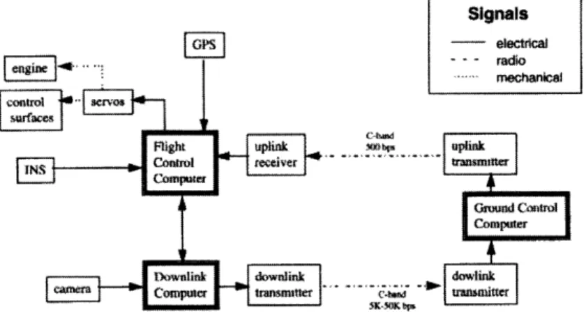
The signal flow diagram for the operational WASP is presented in Figure 3-2.
3.3
Hardware Architecture for the Flight Test
Vehicle (FTV)
3.3.1
Requirements and Constraints
The initial set of requirements for a prototype vehicle included a demonstration of au-tonomous flight, with a minimal requirement to demonstrate that the vehicle can be flown by a remote control pilot, with the help of an onboard stability and control aug-mentation system. Although the FTV uses off-the-shelf electronics its aerodynamic
Signals
- electrcal
- - - radio
... ... mechancal
Rght upik uplik plnk
INS Control recver trmn er
Computer
Downlink downlink dowlink
Conpumtr mtnsinmlner C.nt u er
Figure 3-2: Signal flow for operational WASP
shape is kept as close as possible to the deployed configuration of the operational ve-hicle. FTV is not required to demonstrate deployment mechanisms. The same servo gears and a similar 2 cycle internal combustion engine are used in the FTV. Also, both the FTV and the operational WASP do not have landing gear. The FTV deployment is done from a remotely piloted, powered, ultra-light aircraft; under command from a ground based operator. The retrieval is done by deploying a parachute from the base of the FTV. A digital control system allows tuning of control algorithms in flight and gathering flight test data.
The vehicle was a x1.28 scaled up copy of the operational WASP. The volume constraint was very important for FTV. The allocation of weights inside the FTV was done to keep the dynamics of the flyer similar to that of the operational WASP. The vibrations induced by the engine piston motion and propeller unbalance are important factors in development of the FTV.
3.3.2
Subsystems
Sensors
The inertial measurement unit was chosen to provide high-bandwidth information for the stability augmentation system and attitude information for the autopilot. To
meet the requirement for autonomous flight, the Systron-Donner Motion Pak was chosen. The main performance characteristics of the unit are given in Table 3.2. Mo-tion Pak has analog outputs and requires an A/D card onboard the aircraft to provide an interface to the onboard computer. A mistake was made during the selection of accelerometer full scale ranges: they were chosen to match vehicle dynamics only. As was mentioned in the Section 2.2, it is necessary to choose the full scale of accelerom-eters higher than the vibration level that can be experienced in the vehicle. Because the sensitivity was chosen to be quite high, relative to the vibration created by the engine, the team had to design special anti-vibration mounts to reduce vibration level below .1 g peak-to-peak. These mounts were used to isolate the engine from the nose cone, and the nose cone from the fuselage. However, in spite of the anti-vibration mounts a 100 Hz vibration component, from propeller unbalance, still remained a problem. To fix it, the IMU was mounted on a series of folded rubber sheets. This effectively creates a flexure that acts a fourth order lowpass filter, and guarantees a -80 dB/decade slope at high frequencies. Finally, when saturation of IMU was no longer a problem an active analog low pass filter, with 8 hz bandwidth, was used to filter out residual high frequency vibration. The sampling rate was increased from 50 hz to 100 hz to avoid aliasing.
To achieve autonomous operation, differential GPS was chosen to correct for IMU drifts and provide heading information indirectly. Section 3.7.2 describes an attitude and heading estimation algorithm that uses IMU data and GPS velocity information. The G12 GPS receiver provides 1 m SEP position accuracy and .01 m/sec velocity accuracy in the differential mode. It has a 2 second reacquisition time. The inertial system has sufficient performance to provide adequate navigation during short GPS dropouts.
Communication
Radio modems were chosen to provide two way communication links over a 1 mile range. The modems have serial interfaces, and they are either directly attached to the CPU, or their outputs go through the GPS receiver serial ports.
Computer Stack
A PC-104 stack, described in Section 2.2, was used as the communication bus for the onboard electronics. The stack included a 486DXi 100 MHz CPU from Ampro Computers, a 12 bit A/D card from WinSystems, a power supply from Tri-M engi-neering and ethernet card with boot ROM from Florida DataMation. The 100 MHz processor speed gives a significant advantage in onboard computing power and allows IMU output sampling at more than 100 Hz. By comparison, the 50 MHz processor used in the unmanned helicopter project, described in Chapter 2, could not handle more than a 25 Hz sampling rate, resulting in marginal performance.
The VGA PC104 video card was used in table top testing for troubleshooting of the stack electronics. As mentioned in Section 2.2, it allows one to connect the CPU to a monitor and look at the program outputs directly, not via Ethernet link with ground station computer.
Remote Control Unit
Standard model aircraft remote control servos were chosen to drive the differential stabilizers. The torque requirements, weight and size were the main drivers in the choice of the servos. The Futaba PPM receiver and interface, as described in Sec-tion 2.2, were used to deliver pilot commands to the computer, and for computer commands to the servos.
Retrieval Mechanism
A parachute deployment, to allow safe retrieval of the FTV, is commanded by an RC servo via computer or pilot command.
Power System
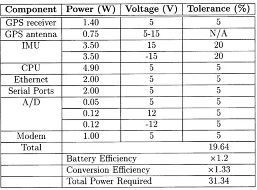
During the process of choosing components special attention was given to minimizing the number of voltage levels used, and the total power requirements as well, so as to minimize battery weight. The complete design of the power system is given in [17].
Table 3.1 lists power requirements for the subsystems.
Component Power (W) Voltage (V) Tolerance (%)
GPS receiver 1.40 5 5 GPS antenna 0.75 5-15 N/A IMU 3.50 15 20 3.50 -15 20 CPU 4.90 5 5 Ethernet 2.00 5 5 Serial Ports 2.00 5 5 A/D 0.05 5 5 0.12 12 5 0.12 -12 5 Modem 1.00 5 5 Total 19.64 Battery Efficiency x 1.2 Conversion Efficiency x 1.33 Total Power Required 31.34 Table 3.1: Power Requirements For Prototype Vehicle
The RC receiver and FPGA draw power from a separate battery. The cards in the PC-104 stack are powered by a PC-104 power supply, which draws voltage in a 10-20 V range from the main battery. The GPS antenna is powered by the receiver.
Figure 3-3 shows the signal flow for the FTV.
3.4
Software Design for the Prototype Vehicle
3.4.1
Functionality
A good software design is essential for system integrity and safety. For example, the prototype vehicle retrieval mechanism is a parachute, and the deployment of the parachute is commanded via the CPU. If the parachute is not deployed the vehicle will be destroyed, and could pose a hazard to people or the environment. An effective and well documented software design increases productivity of the software development, reduces the chances of unpredicted software behavior, and can save considerable
de-Figure 3-3: Signal flow for prototype Vehicle
bugging time and effort. The onboard and ground station software are implemented in the C programming language under the QNX real-time operating system (OS).
One important requirement for system safety is that the parachute should be deployed if one of the following is true:
* pilot commanded deployment
* ground operator commanded deployment * communication link is lost
* RC link is lost
The multitasking capability of QNX OS is used to implement this logic. The pro-gram is split into three processes (Figure 3-4): control, communication, and "watch-dog". The control process functions are:
* read IMU data from A/D card at 100 Hz * read battery voltage from A/D card at 1 Hz
RF modem power system ua
DC-DC convbatteries
RC RX ' AD IMU I ... CPU, M A/D, 4StackAhefmet
engine Onboard systems
Shared Memory 1
Shared Memory 2 Shared Memory 3
Figure 3-4: Software diagram for FTV
* read pilot inputs from receiver interface (serial port) at 5 Hz
* compute control outputs and command them to receiver interface at 50 Hz * perform attitude calculation at 100 Hz
* update parameters in shared memory location 1 (see below) at 5 hz
* control parachute deployment bits in shared memory location 2 (see below) at 10 Hz
The memory location 1 is shared by the communication and control processes. It contains the control system gains, that can be commanded to the communication process by the ground operator, and telemetry information, that the control process gives to the communication process.
The role of the communication process is to
* read requests from ground computer via serial interface with modem
* write requested and default telemetry to modem port * update chute deployment bits in shared memory location 3
The watchdog process has access to shared memory locations 2 and 3. Both contain only 2 bits. The first bit is the command from the other process sharing location to deploy the parachute. The command can come from the pilot through the control process, or from the ground operator through the communication process. The second bit in each location is a health bit. The watchdog process resets both health bits to 0 each time it runs. The other process sets it back to 1. In the event that the health bit remains 0 more than a certain threshold time, the watchdog process deploys the chute.
3.4.2
Implementation Issues
Shared Memory
The use of shared memory can pose a serious danger if not handled properly. Each process, before reading from or writing to a shared memory location, must lock the location, and unlock it after update is made. If this is not done, a race condition may occur in which one process may read data while it is being changed by another process. Thus, the value of the data can be completely erroneous. The FTV shared memory is implemented using "shmemopen" and "mmap" functions of the Watcom C compiler.
Timing
The timing can be done using "signals", which have the same meaning in QNX as in UNIX, or by "proxies", which are QNX versions of interrupt. Each of these requires a per-process timer. The timer is periodically reloaded, and when it expires, it sends either a proxy or a signal, which triggers the run of the process.
In this design, all functions inside a process are run at multiples of the time period the process itself is run. Thus simple counters can be used to trigger the lower rate