BAROTROPIC OR BAROCLINIC INSTABILITY: WHICH IS DOMINANT IN THE UNPREDICTABILITY
OF A 28-VARIABLE ATMOSPHERIC MODEL? by Thomas Francis A.B., Providence 1966 Lavery College
SUBMITTED IN PARTIAL FULFILLMENT OF REQUIREMENTS FOR THE DEGREE OF
MASTER OF SCIENCE
THE
at the
MASSACHUSETTS INSTITUTE OF TECHNOLOGY February 16, 1973
Signature of Author ... ...
Department of Meteorology, 6 February 1973
Certified by....
Thesis Supervisor
Accepted by...
Chairman, Departmental Committee on Graduate Students
y-;
MITLibraries
Document
Services
Room 14-0551 77 Massachusetts Avenue Cambridge, MA 02139 Ph: 617.253.5668 Fax: 617.253.1690 Email: docs@mit.edu http://libraries.mit.edu/docsDISCLAIMER OF QUALITY
Due to the condition of the original material, there are unavoidable
flaws in this reproduction. We have made every effort possible to
provide you with the best copy available. If you are dissatisfied with
this product and find it unusable, please contact Document Services as
soon as possible.
Thank you.
Pg. 10 contains illegible text
I
figures.
.~---
-2-IBAROTROPIC OR BAROCLINIC INSTABILITY: iW-13 IS DOMINANT IN THE UNPREDICTABILITY
OF A 28-VARIABLE ATMOSPHERIC MODEL? by
Thomas Francis Lavery
Snbmzidtt d D tVhe Department of Meteorology on 16 February 1973 im- puEal fulfillment of the requirements for the
degree of Master of Science
ABSTRACT
Dne of the characteristic features of the atmosphere is its an~b .Elty. -zis instability along with observational errors and an imperfect rep-esentation of the governing equations limits the atmosphere's predictability. Both baroclinic and barotropic insta-bility could contribute to this unpredictainsta-bility. A method has
been devised to determine which instability is the dominant factor. This technique is to consider the energetics of uncertainty of a two-layer geostrophic model whose variables have been expanded in Zzmmrated Fourier series. Computation of energy conversion pro-cesses between certain and uncertain components constructed from -two independent smlutions shows that baroclinic instability is the dmrnmanz factor.
'Zhesls Supervisomr: Edward N. Lorenz "Tile: '7roifeDssxr f Meteorology
-3-TABLE OF CONTENTS
I. Introduction 6
A. The Problem 6
B. Two-Layer Model 7
II. The Energetics of Uncertainty 19
A. Derivation of Energy Transformation 19
B. Barotropic Experiment 27
C. Frictionless, Adiabatic Experiment 29 III. Certain-Uncertain Energy in a Baroclinic System 34
IV. Summary and Suggestions 45
References 48
-4-LIST OF FIGURES
1. Two-layer model. 11
2. Certain-uncertain energy diagram. 28
3. Adiabatic, frictionless energy diagram. 30
4. Energy transformations - day 23, first run. 39
5. Energy transformations - day 24, first run. 40
6. Energy transformations - day 3, first run. 41
7. Energy transformations - day 4, first run. 42
-5-LIST OF TABLES 2
1. Value of a.. 15
1
2. Pairs of functions FjFk which interact with
the corresponding interaction coefficient. 18
3. Barotropic energy conversion. 31
4. Energy processes in a frictionless
adiabatic model. 32
5. Energy conversion for 21 "fourth" days. 36 6. Average energy and energy transformation
for four individual days, first run. 43 7. Average e-folding times for energy
transformation for four individual days,
-6-CHAPTER I. INTRODUCTION A. The Problem
Although the atmosphere is not deterministic, the equations commonly used to predict atmospheric variables are assumed to be deterministic, i.e., the present and past states of the variables are assumed to uniquely determine the exact future state. Errors in the observations of the current state of the atmosphere and imperfect knowledge of the governing equations prevent perfect pre-diction of these atmospheric variables. The exact future state cannot be uniquely determined. Also, one distinguishing feature of the atmosphere is its instability. Two time-dependent solutions of the governing equations starting from slightly different initial conditions will eventually diverge and become unrecognizably dif-ferent. In short, atmospheric predictability is limited by the atmosphere's physical instabilities, its inherent non-linear and dissipative character, and by observational errors and imperfectly known physical laws.
Atmospheric instability on the global scale is usually
characterized as baroclinic or barotropic. Growing perturbations receive their energy from the available potential energy of the basic state if the motion is baroclinically unstable, whereas the energy source is the kinetic energy of the basic state if the flow is barotropically unstable. Horizontal wind shear must be present for barotropic instability and vertical shear is require for baro-clinic instability. Atmospheric flow patterns of the global scale are ordinarily barotropically stable but baroclinically
-7-unstable. This has lead to the belief that baroclinic instability is the primary factor in the unpredictability of large-scale atmos-pheric flow.
However, Lorenz (1972), investigating the barotropic insta-bility of Rossby waves which varied with time and longitude,
discovered that perturbations on this basic Rossby flow do grow and that the source of energy for this growth was the eddy kinetic energy of the basic flow. Also, the doubling time for the rms difference between separate solutions was comparable to the growth rate of errors based upon numerical models simulating the general circulation (e.g., Smagorinsky, 1969). These two results suggest that barotropic instability may be the most important factor in the unpredictability in large-scale atmospheric motions.
B. Two-Layer Model
A preliminary investigation of this hypothesis can be per-formed by considering the energy conversions between certain and uncertain energy components in a simple two-layer baroclinic model. The energy flow betwen the energy components will indicate whether baroclinic or barotropic (or both) processes are causing the growth
of errors or uncertainties. The approach will be to consider two separate solutions of a deterministic model, rather than a stochastic dynamic (Epstein, 1969) approach as done by Fleming (1970, 1971a) who first considered certain and uncertain energies.
A simple two-layer model which suits the purpose was developed by Lorenz (1960, 1963, 1965) to study different regimes of flow in
rotating - basin experiments and also to study atmospheric
-8-bility. The basic equations, temporarily neglecting friction and heating, are the geostrophic vorticity and thermodynamic equations
1.1 -J(,) + f
-at ap
1.2
a
V* -E) - - 6at 2 3 ap
where C is the relative vorticity; J is the Jacobian operator with respect to horizontal coordinates, x, y; f is a constant (10 sec
)
Coriolis parameter; w = ap/at where p, the vertical coordinate, is pressure and t is time; and 8 is the potential temperature. The horizontal wind can be decomposed into two components,V= V
where V2 is non-divergent and V3 is irrotational. Thus V
2 -
= k xvYV3 = VX
where Y is a stream function and X a velocity potential; k is the vertical unit vector and V is the horizontal gradient operator. The continuity equation is
2 aw
VX + - 0
These equations are applied to a two-layer model which is diagrammed in Figure 1. Since the equations simulate atmospheric motions, additional terms representing heating and friction must be included. In a two-layer model it is necessary to parameterize the boundary-layer effects in the form of coefficients of heating and friction.
-9-A frictional drag at the surface, proportional to the flow in the
lower layer, and also a drag at the surface separating the layers, proportional to the wind shear, are introduced. Similarly, a heat exchange between the bottom layer and the ground, proportional to the difference between a fixed surface temperature field and the temperature of the lower layer, and a heat exchange coefficient, proportional to the temperature difference of the two layers, are introduced.
Denoting the temperature in the upper and lower layers by
e+
a and 8 - a, the stream functions by T + T and Y - T, and the velocity potentials by -X and X, the governing equations become1.3 -J( Y,V 72) - J(T, 2 7) - k7 2Y + kV 2 T at 2 _ 7
2
2 2 2 1.4 =-J(Y,V T) - J(T,, 2 ) + f2 X + kv 7 - (k+2k')v T ae 21.5 - = -J(Y,) + ovX - he+ h* - (h+2h')a
Here a, the static stability, is taken as a constant. The dependent variables, Y, T and e represent the mean wind, wind shear, and
temperature respectively. The coefficients of friction at the surface and layer interface are k and k' respectively. The coeffi-cients of heating are similarly h and h'; and
e
is the preassigned equilibrium temperature that the surface would assume. The system is closed by the thermal wind relationship2 2
t
e
= AV t
-10-wherAis i rinstant of proportionality.
-n-The present study the governing equations will be used in spectral fIrm. To transform these equations into spectral form l ft 1,.. denote a sequence of dimensionless orthogonal
func-tJ a~aisfy the following conditions:
1.6 V1,. = -L a.F.
1 11
-amlvi i ima ary conditions
-;IBs = 0
1
msm the bar denotes a horizontal average, L is a horizontal length smali., the zelantities a. are dimensionless constants, and 6/as is a
1
- agntial derivative along the boundary. The Jacobian of two nrtIg nal fcamtions satisfy the relation
i.7 12J(F.,F ) = cijk F
i=0
2
S. =L2FiJ(F ,F.)
.ame s~n iess quantities, usually called interaction coefficients, ahich satisfy the relations
e...Z C = = -C = -C =-c
X& jki kij jik ikj kji
-_ _ _ _ -
'ta
,hoose F0 = 1 implying that a0 = 0 and c0jk
Y--~II~---
~--LII
LL--.
--11_--~.-*-~ -XIYYII.~--IX-~ C-_I~
C~-~
LI~C~
-II~-~.
-11-S= 0 -X T+ e + o0 2k' 2 2hE 2k( 2h-0 + 2k( V2 Y -v27) = 0 2h(e - 6 + a) p= 0 p = 250 mb p = 500 mb p = 750 mb p = 1000 mb
-12-for all j and k.
.hsmlig L as a characteristic length scale and f-1 as a unit
of time, Lmrenz (1963) introduces the following expansions for the
dependent variables : i=l 1 ST = L2f T '.F. i=l1 3-11 8= AL2f
f
s.F. , 2 = AL2f E F. 1 i i=l ant3413
V
X
=f
.F.
i=lThe
Aimensionless
coefficients Y., T. and .i' which are functions of1 1 1
time alcne, become the dependent variables of the spectral equations
wdshiria derteyained by substitution of the expansions into 1.3-1.5
S-2( a 2 2 2 -k,j (a -ak)cijk j k j k - k(Yi i k>j -t -2 2 2 -2 1, - (aj -ab)ci(TY k k) - a. k,jj
k>j
-13-1.16 . = (6 - . + w + h( i + 6)
1 kj ijk jk
j
1 1k>j
where the dot represents differentiation with respect to dimension-less time, ft. The thermal wind relation reduces to
1.17 8i = T. if a. 0
1 1
The coefficients of heating and friction h, k, k', and the static stability, a, are dimensionless after division by f.
The thermal wind relationship determines an expression for i.:
1
1.18 . = (a-2 + a)-Z a-2 (aj2-a 2 )c (T.k + k)
k>j
>c..k(8eY.-Y.
ek)
+kQ-T )
-2k'T.+ h(-e.)k,j
J
k>j
To apply these general spectral equations it is necessary to specify the values of the quantities a. and c.ijk. These in turn are deter-mined by the set of orthogonal functions. The choice of the set F. depends upon the geometry of the space domain of the flow. The geometry is chosen to be that of an infinite channel of width TL, having walls at the surfaces y = 0 and y = nL. The flow in the channel is also periodic in the x direction. A suitable set of orthogonal functions is then the set:
-14-Fl = /2 cos(y/L) F2 = 2 cos(x/L)sin(y/L) F3 = 2 cos(2x/L)sin(y/L) F = 2 cos(3x/L)sin(y/L) F5 = 2 sin(x/L)sin(y/L) F6 = 2 sin(2x/L)sin(y/L) F7 = 2 sin(3x/L)sin(y/L) F8 = /2 cos(2y/L) F9 = 2 cos(x/L)sin(2 /L) F10 = 2 cos(2x/L)sin(2y/L) F11 = 2 cos(3x/L)sin(2y/L) F12 = 2 sin(x/L)sin(2y/L) FI3 = 2 sin(2x/L)sin(2y/L) F14 = 2 sin(3x/L)sin(2y/L)
The functions F1 and F8 represent the zonal flow while the remaining functions represent the eddy flow. It is convenient to think of those waves whose arguments are x, 2x, and 3x as wave numbers 2, 4, and 6 respectively.
2
Equation 1.6 is used to determine the a. and their values are1 given in Table 1. The interaction coefficients are determined by 1.8. The method is not so simple. Examples of determining inter-action coefficients for the interinter-action of a zonal wave with two eddy waves and for the interaction of three eddy waves are given below.
The interaction of F8 with one of F5 , F6, F7 and with one of
-15-Table 1. Value of a? 1. 2 i a. 1 1 2 2 3 5 4 10 5 2 6 5 7 10 8 4 9 5 10 8 11 13 12 5 13 8 14 13
-16-F9, F10, F1 1, where the x argument of a pair of eddy functions must
be identical, can be determined from the expression /2 cos 2y J(2 sin nx sin y, 2 cos nx sin 2y)
n = 1, 2, 3 and ignoring L since it vanishes in averaging.
Applying the Jacobian gives
2 2
/2 cos 2y[8n cos nx sin y cos 2y + 8n sin 2nx cos y sin 2y]
Averaging gives
n(f o 2' 2 .2dx
8/2n - 2 I 2n [cos 2nx sin y cos 2y + sin2nx cos y cos 2y] dy dx
64/2n 15
Thus, for example, c8,16 0 15, "
Similarly,
c2,3,12 = 2 cos x sin y J(2cos 2x sin y, 2sin x sin 2y)
= -32 sin x cos x sin 2x sin2y cos 2y
-8 cos2x cos 2x sin y cos y sin 2y
22
6r sin x cos x sin 2x sin2y cos 2y dy dx
4 2 2
= - S
f
cos x cos 2x sin y cos y sin 2y T 00
= 2 - 0.5
= 1.5
-17-The non-zero interaction coefficients and the respective pairs of functions which interact with each function are listed in Table 2.
In summary, the quasi-geostrophic equations have been used to describe thermally forced rotating flow in an infinite channel. Gravity and sound waves have been filtered from the solutions. The model also omits the transport of momentum by the vertical motions and by the divergent part of the wind. However, the transport of heat by the total horizontal and vertical motions is still included. Kinetic energy is dissipated by internal and surface friction.
There is no vertical velocity at the top and bottom of the model and no exchange of heat and momentum through the sides of the channel.
The numerical integration scheme used to solve the spectral equations is a 4-cycle scheme developed by Lorenz (1971).
-18-Table 2.
Pairs of Functions Fj Fk which Interact with Fi and the Corresponding Interaction Coefficients
C = -8 31t i F.F /C. .j k ijk 1 2 5 3 6 4 7 9 12 10 13 11 14 C 2C 3C 0.8C 1.6C 2 5 1 12 8 3 12 3 14 4 13 C 1.6C 1.5 0.5 2.0 3 6 1 13 8 12 2 14 2 4 12 2C 3.2C 1.5 0.5 2.5 4 7 1 14 8 13 2 12 3 5 10 3C 4.8C 2.0 2.5 -2.0 5 1 2 9 8 9 3 11 3 10 4 C -1.6C -1.5 0.5, -2.0 6 13 108 92 2C -3.2C -1.5 11 2 94 -0.5, -2.5 1.4C 69 6 11 7 10 -1.5 -0.5 -2.0 5 9 5 11 7 9 -1.5 0.5 -2.5 69 -2.5 6 12 6 14 7 13 1.5 -0.5 2.0 12 5 14 5 7 12 1.5 -0.5 2.5 7 1 4 11 8 10 2 9 3 13 5 3C -4.8C -2.0 -2.5 2.0 12 6 2.5 8 2 12 3 13 4 14 5 9 6 10 7 11 -1.6C 3.2C 4.8C -4.8C -3.2C -4.8C 9 121 85 26 35 3 7 0.8C -1.6C -1.5 -1.5 -2.5 10 13 1 8 6 2 7 4 5 1.6C -3.2C -2.0 -2.0 11 14 1 8 7 2 6 3 5 1.4C -4.8C -0.5 0.5 12 19 82 23 34 0.8C 1.6C 1.5 2.5 13 1 10 8 3 2 4 5 7 1.6C 3.2C 2.0 2.0-14 1 11 8 4 2 3 5 6 1.4C 4.8C 0.5 -0.5 5 6 1.5 46 -2.5 6 7 2.5
-19-CHAPTER II. THE ENERGETICS OF UNCERTAINTY
A. Derivation of Energy Transformation
The adiabatic frictionless version of the two-layer model con-serves the quantity
a+ l1
i i
where
2.1 k = a2 2)+
i1 1 1
is the dimensionless kinetic energy, and
2.2 A = 1 6
i
is the dimensionless available potential energy.
Studies of the general circulation of the atmosphere often con-sider energy conversions between zonal and eddy components of kinetic and available potential energy. Similarly, Fleming (1970, 1971a) considered conversions between certaif and uncertain components of kinetic and available potential energy in his study of stochastic
dynamic prediction.
In this study conversions between certain and uncertain energies are also calculated, but not in a stochastic dynamic context.
Starting from arbitrary initial conditions, the model is run for a few weeks to eliminate the transient effects of the initial conditions; and then a random perturbation is added to each predicted dependent variable to define a second solution. The model is then integrated with two solutions. Certain and uncertain variables are defined
-20-from the two separate solutions.
If Y and 2. are the i-th components of the stream function
1 2
i i
from the original and perturbed solutions respectively, then the certain component is defined as
T1.+
2.
c.
2
and the uncertain component is
1. 2.
u. 2
since T = L2f'iY., then i 1 YI + \Y2 c 2 and 1 2 u 2 where Y 1 = L 2 f and 2 = L 2 f 2. 1 1 2 2 Similarly, T 2 c 2 u- 2 2l+ 82
E
-u 2
These are defined in this manner so that the total certain energy plus the total uncertain energy equal the sum of the energies of the
-21-two solutions. For example,
A =
A +
A -
(9e
*1V
+
17
eV
)
c U a c C U U 4a ( 1 +62)*7 ' 1E
-
2)
S
(E
. 11
+ve
e
2)
= A1 + A2. Similarly, K = Kc + Ku = K1+ K 2To derive expressions for the conversion, generation, and dis-sipation of certain and uncertain energy, it is convenient to con-sider the governing equations for the certain and uncertain variables before expansion into spectral form. These equations are:
2.3
-~-
= -J(c'c6 )
-
J(
,9
) + a6
6t c c c u u c
2.4 -8 = -J( ) - J( ) +
2 2 2 2 2
2.5 ; Yc =-J(Y c c, ) - J(u ' 2~u ) - J(Tc,7 c) - J(Tu ,VT u)
6 2 2 2 2 2.6 T7 = -J(T , ) - J(Y ,7 u) - J(T V ) -J(T u,2uY ) + f6 c _ 2 2 2 2 2 2.7
-
= -J(,v'Y
U) - J(Tv ') - J(T , T)
t c u U c C U U c II --..l-.;----r-1.L I ~^illlj~LIUII
-22-2.8 2 2 2
bt u c u U c c U
2
-J( ,V2' C) + f6
where 6 = 2t and 6 = V 72 and where friction and heating are
C C U U
temporarily neglected.
Multiplication of 2.3 by
ec
and by -1 , and taking the hori-zontal average gives an expression for the time rate of change of certain available potential energy:2.9 1 b 2 - 6 J(/
,6
)
- 6 J(Y
, +6 6)/a
20
at
c c c c c u c ccfSimilarly,
2.10
1
= (
J(
,e
) -
J(
,
) +
o6
e)
20 at c U U U c
is the change in uncertain available potential energy. The time derivative of K can be written as
c
1 a
{VY
* YVlY + VT VTc 2 at c c c c which equals b 2 a 2 cat
c c 6t cMultiplication of 2.5 by
Yc
and 2.6 by Tc and substitution into the above expression results in the time change of certain kinetic energy:Kc 2 2 2 2.11 = Y (Y ,V 2) + Y J( , 7 ) + Y J( ,VT ) 2t c c c c u u c c c 2 + Y J(T ,V T
)
c u u~--~- -23-2 2 2 + cJQ ( , T ) + T J( u'I T u) + T J(T c T 2 + T J(T 7)7, + fT 6 Similarly, 2.12 2t -K u = 2 at VY u u*VY u + VT *VTU = -- y -V2 y 7 T T u 6t U u at U 2 2 2 u c u u u cJ (T c2V u 2 2 2 2 2 + T J(T c,v2 U) + T J(T U,12Y) + ftu 6
Let C(X,Y) refer to the conversion of X into Y. Recognizing that
2 2 2 2 = T J (T 2u, c ) = 0 and that 2 2 Y cJ(T c ,'V ) + T J(Yc , 'cVT 2 2 = YJ(u9 , T ) + T J(Yu , ) = 0
the energy conversion rates are:
-1 -1
-24-2.14 C(A ,K ) 2.15 C(Au,Ku) 2.16 C(K c,Ku)
-6
E
c c = - 68 uu 2 2 2 = cJ( u , u) " Yc J (c uu , ' Tu) Tc - 7cJ(u c ,v ) u u 2 2 2 - J(T ( Y + u J(Tc , T )c
cru'
)u
+ TUJ( ,JTU ) + TuJ(c,2 )Considering the friction and heating terms in the equations for the evolution of the certain and uncertain variables gives the energy generation and dissipation.
at c c c 2.18 -V2Y = ... k(V - 2 T) 2.18 t u u v u
a
2 2 2 2.19 -V 2 = ... k - (k + 2k')V T at c c c 2.20 a V27 ... k2kV - (k + 2k')V7 at u u u 2.21 8 h[ - ( - ) at c c 2.22 t u 8- u = ...- h(fu u - a) ,assuming there is no forcing on the uncertain temperature field. Proceeding as in the derivation of the conversions, the following expressions result:
2.232 YC 2 c 2 2
2.23 D(K ) = k (V2~ - ) - k7 V + (k + 2k') T7V 7T
-25-2.24 D(K ) = kY (V2 -27 ) - k7 V2u + (k + 2k') .V 27T
2.25 G(A
)
= (h 6e - he)
2.26 G(A) = -(he2 >
u u
where D represents dissipation and G represents generation.
These expressions for the generation, conversion, and dissipa-tion of certain and uncertain energies are also converted into spec-tral form. The procedure is simply to substitute the expansions for the certain and uncertain variables into 2.13 to 2.16 and into 2.23 to 2.26, and to apply the relations 1.6 to 1.8, which govern the set of orthogonal functions.
First, consider -1
C(A , A) =
a
8 J(Y ,u )
c i c 1Y =FY
F.
u u. 1 i 1eu =
e
F.
u U. 1 1 1(ignoring the dimensional constants). Substituting the expansions into C(A ,A ) gives
C U
C
(A
,A)
=a-1e
F
J(E
F.,
6)
Su i .u Fk)
i 1
J
jk
k
-26-S-1
c,[
E Yu J(F. Fk
i i j,k j k but -2 J(Fj,Fk) = L- 2 c ijkFi -1 . C(A,A) = a c. F.F. 6 $ 1 U Uk i,j,k I ] k Sij k 0 Tu. i,j,k C j Uk -2since F.F. = 6.. = 1, (and ignoring the L in the substitution above).
i i 11
Hence, the conversion between (dimensionless) certain and uncertain available potential energy is
2.27 C(A,A ) = 1 Z i c u a ijk c. uj u Similarly, 2.28 C(A ,K ) =-W TC c c c. c. 1 1
2.29
C(A
,K )
=
-Zuw
u u u. u. 1 1 2.30 C(K ,K ) = + ac + T T + T c ua k ( ci u j u k ccui uju k ci uj u k + T u k )The spectral forms of the generation and dissipation of available and kinetic energies are:
-27-2.31 G(A ) = hlea (: * - ) c c I c 1 i
2.32
G(A )
=
-h
e 82
U U. 1 2.33 D(Kc) = k a 2 - 2k a 2 Y T + (k + 2k')me 2 c 1 C. i C. C. C. 1 1 1 12.34 D(Ku) = kZa2 2 - 2k a2Y T + (k + 2k') 2
1 1 1 1
where h, k', and c are all dimensionless coefficients.
B. Barotropic Experiment
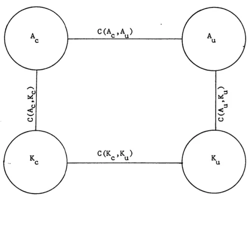
The energy generations, conversions, and dissipations of the baroclinic two-layer model are indicated in an energy diagram shown in Figure 2. The energy flow characterized by this diagram will be shown in numerical calculations. These calculations will give a preliminary indication of whether baroclinic or barotropic pro-cesses are dominant in the growth of uncertainties or errors in the unpredictability of the model. If the growth of uncertain energy is mainly through a conversion of Ac into Au, then baroclinic insta-bility dominates. If the growth of uncertainty is primarily via a conversion of Kc into Ku, then barotropic instability dominates. This is the crux of the numerical experiment.
Before a proper numerical experiment can be performed, it is necessary to test the model. Fortunately, there are physical situ-ations in which the numerical calculsitu-ations will give predictable results. This verifies that the energy transformations have been
-28-G(A ) G(A ) C (A cu~,A u) 0 C (K ,K )cu D (Kc
)
D (K )Figure 2. Certain-Uncertain Energy Diagram. II~l-LIIPltlls~
-29-derived correctly and also that the computer program is correct. The simplest case to consider is a barotropic experiment in which all the 7. and
e.
and all the friction and heating terms are1 1
set equal to zero. The energy diagram reduces to the bottom of Figure 2. Here energy can only be converted between certain and uncertain kinetic energies; and hence this experiment serves as a
test of the derived formula for C(K ,K ). Table 3 shows the results for an integration over 15 hours. It is seen that the total energy is conserved. The important result is that the
energy conversion rate at a particular time step equals the average of the actual change in Ku taken from the preceeding to the following time step. This indeed verifies that the expression for C(K ,K )
is correct. Also, subsequent integration of the barotropic model over a time period of six weeks showed that the total kinetic energy was conserved to about seven parts in 10,000.
C. Frictionless, Adiabatic Experiment
A more complex model results if the i. and B. are retained. The linear and constant terms are still zero. This is the fric-tionless adiabatic model. Figure 3 is the corresponding energy diagram -- here the sum of the kinetic and available potential energy is constant with time.
The model was run throughout a day in three hour time steps to validate the derivation of the other energy conversions. The
results are shown in Table 4. In this experiment the random per-turbation added to the first solution was of the order 10-4 . Since turbation added to the first solution was of the order 10 .Since
-30-Figure 3. Adiabatic, Frictionless Energy Diagram.
_II~L~II~---~
ILY--l-~l~ ll~ ^---Lllillllll i-tilll-.~-~ ~-~~L-- -~I^~-~~1~- -~ U~---~ -IIII
-31-Table 3.
BAROTROPIC ENERGY CONVERSION
Time Total Energy K K A Ku K C(KcK
(hrs) (x10 - 2 (x10 2 ) (10- 6) (10 ) (10 ) (10 ) 3 0.2262 .22619 .11316 - .24 6 0.2262 .22619 .11292 -.045 -.048 + .15 9 0.2262 .22619 .11307 .36 .358 .57 12 0.2262 .22619 .11364 .79 .791 1.02 15 0.2262 .22619 .11466
- represents an average over two time steps.
the uncertain energy is four orders of magnitude less than the certain energy, C(A ,A) < < C(A ,K ); and consequently it is possible to
c u c c
isolate C(A c,K c ) in the same way as C(Kc ,K ) was tested in the
baro-tropic experiment. Table 4 indicates that the conversion of certain available energy into certain kinetic energy at a particular time
step equals the average of the actual change in Kc (or A c) taken from the preceeding to the following time step. This verifies that the derivation of C(Ac ,Kc ) is correct.
Since the other three conversion rates are about the same, it is not possible to isolate them in the manner described above. However, it is still possible to check the derivations since C(Kc ,Ku) + C(A,Ku) should approximately equal the average actual change in K . Similarly, C(A ,A ) - C(A ,K ) should approximately
equal the average actual change in A . This is indeed the case. For example, consider the energy processes between hours 9 and 15.
ENERGY PROCESSES K AK c c x10- 2 x10- 4 .3485 .3510 .3544 .3588 .3642 .3707 .3783 .3871 0 .25 .34 .44 .54 .65 .76 .88 Table 4.
IN A FRICTIONLESS ADIABATIC MODEL
C(Ac ,K) C(A ,A ) C(Au,K )
x10- 4 x10-8 x10- 8 .193 .292 .391 .492 .596 .704 .817 .936 .908 1.976 3.159 4.451 5.881 7.522 9.395 11.563 .604 1.124 1.654 2.211 2.810 3.170 4.210 5.055 A c 10-1 xlO .2667 .2664 .2661 .2657 .2651 .2645 .2637 .2628 A u x10-6 .450 .457 .471 .491 .519 .557 .604 .664 C(K ,K ) 10-8 xl0 K u x10-6 .231 .240 .255 .267 .304 .340 .384 .437 TE 10-1 xlO .020 .086 .158 .242 .345 .477 .654 .860 .3016 .3016 .3016 .3016 .3016 .3016 .3016 .3016
-33-AK .245 x 10- 7 u &A , .242 x 10- 7 u At hour 12 -7 C(Kc,K ) = .024 x 107 C(A ,K ) = .221 x 10- 7 C(A ,A ) = .445 x 10 - 7 Cu Thus, AK C(K ,K )+ C(A ,K ) A C(A ,A ) - C(A ,Ku)
-34-CHAPTER III. CERTAIN-UNCERTAIN ENERGY IN A BAROCLINIC SYSTEM
The choice of the values of the heating and friction coeffi-cients as well as the value of a will determine the type of motion
that evolves. Since the purpose of this thesis is to test the dominance of barotropic or baroalinic instability in the unpredict-ability of the atmosphere, it is desirable to choose parameters that give irregular nonperiodic flow that resembles atmospheric motions. This has been achieved by using the values
e
= 0.07031 h = 0.11718, and a = 0.03906. The rest of thee.
were zero. This forcing in only the first zonal component represents heating at the equator and cooling at the poles. Also, following Lorenz (1963), h = k = 2k'.Although the motion that evolved was irregular and nonperiodic, the components representing wave number 6 were more unstable than the other components. Consequently, these components were more developed than the others; and most of the energy of the system was contained in the zonal flow and wave number 6. This is unrealistic in simulating atmospheric motions and is a weakness in the experi-ment. Changing the values of the external parameters could not eliminate this bias.
To test the dominance of baroclinic or barotropic instability the following procedure was devised. The model was run for 52 days using initial data generated from a run with arbitrary initial conditions. At the first time step a random perturbation was added to all the independent variables; and the two solutions were
inte-
-35-grated simultaneously for four days. Since the two solutions rapidly diverge during the first two days, it seems that the energy conversions during the fourth day are most representative of the growth of uncertain energy. At the end of the fourth day the per-turbed solution was terminated and the original solution was then integrated separately. On the ninth day the original solution was again perturbed and the procedure was repeated. The procedure was performed seven times during the 52 day period. The 52 day run was repeated to investigate any effect of the random perturbation scheme. Finally, the test was run with the first perturbation
added on the third day; and the total time was extended for two extra days. The entire procedure produced output for a total of 21 "fourth" days, seven from each 52 day integration. Table 5 lists C(Ac ,Au) and C(K c,K ) and C(A ,K ) for the 21 days.
The results are quite conclusive. The growth of uncertainty in this simple, two-layer model is dominated by baroclinic instability. Although there is some contribution from the barotropic process,
C(A c,A ) is greater than C(K c,K ) throughout the entire experiment. It is generally an order of magnitude greater and in 4 cases contri-butes all of the energy since C(K c,K ) is negative in these cases. Also, it is seen that most of the uncertain kinetic energy is
ultimately produced from Ac via the two conversion processes C(A c,A )
and then C(Au Ku).
The first fourteen conversions represent essentially the same synoptic situation -- the first seven emanated from a slightly dif-ferent perturbation scheme than used for the second seven. As
-36-Table 5.
ENERGY CONVERSIONS FOR 21 "FOURTH" DAYS
C (Kc ,K ) x10-5 0.15701 0.38178 -0.00285 0.09282 0.09189 -0.01355 0.07291 0.15727 0.38050 -0.00368 0.09268 0.09237 0.14302 0.25109 -0.00061 0.08899 0.16468 -0.01293 0.06653 C(A ,Ac uu ) x10-5 C(A ,K ) u u 10-5 xl0 1.23450 3.15130 2.74760 0.76799 0.68620 4.53140 0.95686 1.23220 3.13990 2.73820 0.76498 0.68167 1.38610 2.63810 3.58120 0.80488 0.75169 4.89290 1.00460 0.65730 1.56170 1.40070 0.42162 0.35827 2.29290 0.53678 0.65776 1.55540 1.39550 0.41990 0.35602 0.74639 1.29910 1.82370 0.44535 0.38650 2.47240 0.56732
1I1LII--LI-^L-iII__-.-.---
-37-Table 5 indicates, the results are basically the same for the two runs. The last seven conversions represent a different synoptic situation in that the perturbation scheme commenced on the third day rather than the first day of the 56 day run. Here the pattern
is different, yet baroclinic instability still dominates.
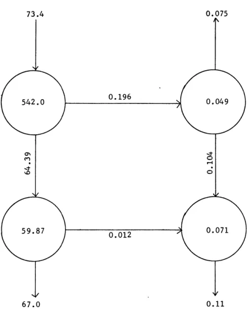
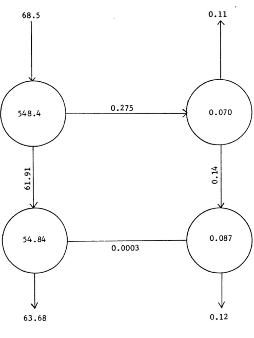
A better picture of the certain-uncertain energy transformation process can be seen in Figures 4 and 5. Figure 4 diagrams the energy processes on the 23rd day of the first 52 day run. Figure 5 represents the energy transformations on the 24th day, corresponding to the third "fourth" day listed in Table 5. On day 23 both baro-clinic and barotropic processes are contributing to the growth of uncertain energy; but on the next day baroclinic instability is the only contributor. This is reflected by a large increase in Au with only a small increase in K and an actual flow from K to K on day 24. The maintenance of K is through C(A ,K ). Figures 6 and 7 show a more typical example. Figures 6 and 7 represent days three and four, respectively, of the first run. On both days both pro-cesses contribute with the baroclinic instability process dominating.
A further insight into the dominance of the baroclinic processes can be gained by considering the growth rates of uncertain available and kinetic energies averaged over the first 52-day run for four individual days. Table 6 gives the average uncertain energies and
their corresponding energy transformations. Table 7 lists the
e-folding times for the various conversions considered separately and in different combinations. As the latter table indicates, the growth of both A and K via a baroclinic conversion, considered asu u
-38-if it were a separate process, is explosive -- with doubling times of much less than 24 hours for all four days. The growth of uncertain kinetic energy via the barotropic process, C(K ,K ), is much slower. On day 1 Ku actually decreases. Days 3-4 have
e-folding times of greater than 4.5 days.
The e-folding times resulting from a combination of the two processes are again quite short. Other than on the first day, these times are less than one day. This shows how the baroclinic processes completely negate the effect of C(Kc,Ku). It is necessary to include G(A ) and D(K ) to produce the more realistic e-folding times found in the total system.
In summary, baroclinic instability is the primary mechanism in causing the unpredictability of the two-layer quasi-geostrophic model.
-39-73.4
0.196
0.012
67.0 0.11
Figure 4. Energy transformations - day 23, first run. All numbers are to be multiplied by 10-4 .
III_____I*IOLI~ML'I~^LIY114CX- L~~-l~l_ Ipll ^.--~-11-*ll~L_---^1~PII-~ ---- _^ _-~ -_L~Y-r(~--*- ~---~I^-_
-40-68.5 0.11 0.275 48.4 0.275 0.070 54.8400 0.087
0.0003
63.68 0.12Figure 5. Energy transformations - day 24, first run. All numbers are to be multiplied by 10.-4 All numbers are to be multiplied by 10.
*--
-41-0.025
83.5 0.035
Energy transformations - day 3, first run. All numbers are to be multiplied by 10-4.
All numbers are to be multiplied by
10-76.3
Figure 6.
-42-0.045
87.61 0.062
Energy transformations - day 4, first run. All numbers are to be multiplied by 10-4.
All numbers are to be multiplied by 10-83.07
Figure 7.
-43-Table 6.
AVERAGE ENERGY AND ENERGY TRANSFORMATIONS FOR FOUR DAYS, FIRST RUN
All numbers are to be multiplied by 10-5 All numbers are to be multiplied by 10.
K A u u 0.494 0.161 0.398 0.229 0.483 0.337 0.693 0.513 C(Ac,A) C (A ,K ) C(Kc,K ) G(A ) cuU U G(A)u 0.505 0.984 1.311 0.384 0.554 0.672 -0.145 0.019 0.107 2.011 1.032 0.111 D(K ) u± -0.373 1.817 -0.374 0.647 -0.520 0.686 -0.807 0.932 uL~C~L.- li li-i- ---L~LL~~-^_I~1L i
-44-Table 7.
AVERAGE E-FOLDING TIMES FOR
ENERGY TRANSFORMATION FOR FOUR DAYS, FIRST RUN Time units are days.
A U 3 C(A ,A )-C(A ,K
)
1.330 0.533 0.529 0.524 K u C(A ,K)
1.29 0.72 0.72 0.67C(A , A )-C(A ,K )+G(A) c u u u U -1.06 4.09 3.07 2.98 K 3 4 K K u u C(K ,K )+C(A ,K ) C(K ,K )+C(A ,K )-D(K ) c u U u c u U U U 2.630 0.695 0.620 0.606 -0.313 -5.380 5.200 3.260 1 Baroclinic growth. Barotropic growth.
Baroclinic and barotropic processes considered together. Inclusion of generation and dissipation.
A U C(A ,A cu ) 0.318 0.232 0.258 0.256 K 2 U C(K ,K ) -3.31 21.00 4.52 6.24
-45-CHAPTER IV. SUMMARY AND SUGGESTIONS
Barotropic and baroclinic instability may both contribute to the unpredictability of the atmosphere. A procedure was developed to determine which instability is the primary factor. Following Lorenz (1965) a 28-variable atmospheric model was developed by
expanding the equations of a two-layer geostrophic model in truncated Fourier series. By defining certain and uncertain components as
half the sum and difference, respectively, of two separate solutions generated from slightly different initial conditions, energy con-version rates between certain and uncertain energies were studied.
It was found that the conversion between certain available potential energy and uncertain available potential energy was the greatest source process for uncertain energy. This indicates that, at least, the unpredictability of the model is a result of the baroclinic in-stability process.
As Robinson (1967) suggests, predictability experiments using atmospheric models may tell more about the model than the atmosphere itself. Obviously, a simple, two-layer model is but a crude repre-sentation of the atmosphere. One serious limitation is that the model equations were truncated at wave number 6. Probably more
emphatic results would have been produced if more wave numbers were included. Yet more important, however, is the limitation that the eddy kinetic energy was primarily contained in wave number six.
Since wave number 6 includes synoptic scale disturbances -- which are baroclinically unstable -- our results could be biased in favor of
-46-baroclinic instability.
Lorenz' suggestion (1972) that barotropic instability is the most important factor in the unpredictability of large-scale atmos-pheric flow was based on an analytical study of Rossby's solution of
the barotropic vorticity equation. Because his result was analytical, it was not dependent on the choice of finite-differencing schemes, horizontal resolution, etc. In short, it was not dependent on any numerical procedure. The serious limitations of the two-layer model and Lorenz' analytical result seem to indicate that the con-clusions of this thesis are certainly not definitive.
Using a more sophisticated numerical atmospheric model, of course, is a possible extension of this study. Certain and uncer-tain energy can readily be defined if the available potential energy of the model is quadratic, e.g., geostrophic or some simple primitive equation "shallow water" model. If the available potential energy is not quadratic, it is not clear how to define the certain and uncertain forms of energy. If the available potential energy is proportional to the temperature variance on an isentropic surface as in the real atmosphere, it may not be possible to formulate the energetics of uncertainty.
A stochastic dynamic prediction model may be the next logical step. For example, Fleming (1970, 1971a, 1971b) developed a sto-chastic dynamic model from the two-layer model described in this study. He actually derived an equation for the evolution of the ensemble
variance -- the measure of uncertainty in the model. The advantage _~_/l___~_*__ Uln/r__~___l *~_~(X~_VY_~
-47-of this approach is that the uncertain energy does not increase without limit as in a deterministic prediction. This seems to be more representative of the real atmosphere. Ultimately, the
pro-blem may be considered using a stochastic dynamic version of a global primitive equation model.
-48-REFERENCES
Epstein, E. S., 1969: "Stochastic dynamic prediction." Tellus, 21, 739-757.
Fleming, R. J., 1970: Concepts and implications of stochastic pre-diction, NCAR Cooperative Thesis No. 22, 171 pp.
Fleming, R. J., 1971a: On stochastic dynamic prediction: I. The energetics of uncertainty and the question of closure. Mon. Wea. Rev., 99, 851-872.
Fleming, R. J., 1971b: On stochastic dynamic prediction: II. Pre-dictability and utility. Mon. Wea. Rev., 927-938.
Lorenz, E. N., 1960: Energy and numerical weather prediction. Tellus, 12, 364-373.
Lorenz, E. N., 1963: The mechanics of vacillation. J. Atmos. Sci., 20, 448-464.
Lorenz, E. N., 1965: A study of the predictability of a 28-variable atmospheric model. Tellus, 17, 321-333.
Lorenz, E. N., 1971: An N-cycle time-differencing scheme for step-wise numerical integration. Mon. Wea. Rev., 99, 644-648. Lorenz, E. N., 1972: Barotropic instability of Rossby wave motion.
J. Atmos. Sci., 29, 258-264.
Robinson, G. D., 1967: "Some current projects for global meteoro-logical observation and experiment." Quart. J. Roy. Meteor. Soc., 93, 409-418.
Smagorinsky, J., 1969: Problems and promises of deterministic extended range forecasting. Bull. A. M. S., 50, 286-311. I-~~--sUIIYY---~^-I PIC. -^----~lilU-..l ~Y ~IY)I~LLC-Y~-CI-lC11111
-49-ACKNOWLEDGEMENTS
I simply wish to thank Professor Edward N. Lorenz without whose assistance this thesis would not have been possible.
I--.~_^ I~n.^l-LI-~L-'(I -L~'~1 1111-11111. ) L---lli Y IC~--1II~--- I1~L