An aggregate model of petroleum production capacity and supply forecasting

AND SUPPLY FORECASTING by

M. A. Adelman and James L. Paddock Energy Laboratory

Working Paper No. MIT-EL 79-005WP Revised:_{January 1980}

I

Mf' 7iES

J UN 0 3 1980

1i.. ..1).

AN AGGREGATE MODEL OF PETROLEUM PRODUCTION CAPACITY AND SUPPLY FORECASTING*

by

M. A. Adelman and James L. Paddock ABSTRACT

This paper presents a complete discussion and documentation of the M.I.T. World Oil Project Aggregate Supply Model. First, the theoretical

development and methodology are presented. The relationships between geologic and economic characteristics are analyzed and a system of equations representing the inertial process model are derived.

Next, the construction of the data is described and the data, by country segment, is presented in detail. Methods of bridging the many gaps in the data are discussed.

Finally, the simulation forecasts of the model are presented through 1990.

*This research has been supported by the National Science Foundation under Grant No. DAR 78-19044. However, any opinions, findings,

conclusions or recommendations expressed herein are those of the authors and do not necessarily reflect the views of NSF. The work also is supported by the M.I.T. Center for Energy Policy Research.

We wish to thank the following individuals for their comments on earlier drafts: P. Eckbo, H. Jacoby, R. Pindyck, J. Smith, and M. Zimmerman. Also, for research assistance and help in data analysis we thank J. Carson, W. Christian, D. McDonald, H. Owsley, G. Ward, and, in particular, A. Sterling. For editing and typing we are grateful to S. Mehta and A. Sanderson.

07:S:1851

V

Alka l ."I

2

Table of Contents

Page

1. Aggregate Supply Model 3

1.1 Analysis of Reserve Additions 3

1.2 Production Profile of Reserve Additions 7 1.3 Estimation of Additional Productive Capacity 9 1.4 Historical Production-Reserve Ratio 12

1.5 Optimal Depletion Rate 15

1.6 Analysis of Capital Costs 22

1.6.1 Constant Capital Coefficients 22 1.6.2 Variable Capital Coefficients 29

1.7 An Example -- Mexico Reforma 34

1.8 The Influence of Taxes on the Depletion Rate 38

1.9 Conclusion 40

2. Data 41

2.1 Production and Reserves 41

3. Production Capacity Forecasts 48

4. Areas for Further Research 56

4.1 Reserves Added 56 4.2 Depletion Rate 57 Appendix I 58 Appendix II 60 References 61 _._. ._._I . ..

.,.--1. Aggregate Supply Model

The objective of the model developed here is to forecast crude oil production capacity by geographical area. The forecasting method is based on projections of development rig activity and analysis of returns to drilling. Returns calculated as proved reserves-added are superior in theory, and we discuss them first; but in almost every case we will need to use the second-best method: wells drilled per rig-year and productive capacity per well.

1.1 Analysis of Reserve Additions

As used by the American Petroleum Institute (API) the concept of proved reservesl has a definite economic meaning: a highly accurate forecast of what will be produced from wells and facilities already installed. Since variable costs are normally only a small part of the total, it would take an unusually severe price drop or cost increase to abort much production from proved reserves.

Given an estimate of current proved reserves, we must next develop a method for forecasting changes in this quantity. We consider gross

additions to proved reserves in any year as an output, and rig-years as a proxy or indicator of investment (capital) input which generates these reserves. Let Rt be proved reserves in an area at the end of year t; Qt be the area's crude oil production; and RYt be the available number of operating rig years. The reserves-added per rig-time unit, RA, are calculated as:

Outside the U.S., published "proved reserve" estimates generally include a substantial element of what the API calls "indicated additional reserves from known reservoirs," and also some "probable reserves." See Adelman-Jacoby (2), p. 34, and Adelman-Houghton-Kaufman-Zimmerman (1),

Chapters 1 and 2, for a more detailed discussion and an example of aborted reserves.

4

75 75

RA = (R₇₅ -R ₇₂ + Qt)/( RYt) (1)

t=73 t=73

where 1973-1975 is assumed to be a reasonable base period for estimation. (More recent data are substituted as they become

available.) The numerator in (1) is gross additions to proved reserves over the 3-year period, end-1972 to end-1975, where additions include proved new-field discoveries, new pool discoveries, and revisions and extensions of known fields, often from development drilling. The

denominator is the number of rig-years during the same period. Rig-time is superior to feet drilled because it is a better proxy for investment, although it is necessary to calculate RA separately for onshore and

offshore areas due to their differences in required fixed investment. We thus divide the countries analyzed into onshore and offshore. Rig-time registers all time-related elements, including not only depth but also time used in moving rigs; interruptions for lack of an essential part or service or any other reason; unusually difficult drilling conditions, etc.

Equation (1) applied to a subsequent year's drilling rate yields a forecast of reserve additions:

aRt = (RYt) (RA) (2)

The method is a simple extrapolation of recent (1973-1975) experience, with only inertia (which is considerable) to justify its use. We currently use RA, as calculated in (1), as an exogenous constant in the model. Thus, for example, the effect of higher prices on supply makes

itself felt only by increasing investment, i.e., drilling. A later paper will endogenize development drilling.

Of course the yield from new investment cannot go on forever, undiminished by the effects of depletion. Thus we define a depletion

--- 7 ·I---I-- ----P---'

coefficient, bt, which builds in a diminishing return to further

drilling. Let Cum Rt encompass all past production plus current proved reserves in _{year t. Ultimate recoverable reserves, Ult Rt, are then} Cum Rt plus all future additions to proved reserves (and ultimately, therefore, to production). Using 1975 as the base year for reserves data, bt may be defined as:

Cum Rt Cum R

bt = (1- t )/(1

l

-

t

t 75

The expression for reserve additions, equation (2), is now modified to take this depletion factor into account:

ARt = (RYt) (RA) (bt) (4)

As new reserves are created by drilling, they are essentially a transfer from the total pool of ultimate production, Ult Rt, for the country or area. Obviously our numerator in (3) is designed to be sensitive to intertemporal reestimations of Ult R, in response both to new discoveries and to new technologies, etc. Currently we assume

Ult Rt t Ult R75, thus bt falls each year (from an initial value of unity

when t = 1975) so that Rt is less and less each year for a constant drilling rate. Thus, if cumulative production plus the amount already

impounded into proved reserves at year t were the same as the ultimate production, then (Cum Rt)/(Ult Rt) in the numerator of Equation (3) would be unity, bt would therefore be zero, and no amount of drilling could add anything to proved reserves in (4). The closer the numerator of (3) is to zero, the smaller is the fraction, and therefore the less is the return to drilling effort, relative to the 1973-75 showing.2 _As

2

For a fixed Ult Rt (i.e., no major change in the ultimate

prospect) the "discovery decline" is linear. As Cum Rt goes from Cum R75 to Ult Rt, bt goes (linearly) from one to zero.

6

the ultimate reserve estimates are changed up or down, or if we are

confronted with varying estimates of ultimate reserves, we can substitute them into Equation (3) and see what difference it makes in our forecast. For example, if technological development causes an increase in Ult Rt in some year t > 1975 then bt may be > 1 and RA will capture the increased return to investment.

Our definition of Ult R includes expected discoveries. Our model does not now have an explicit exploration and discovery process. This process is implicitly imbedded in our reserves additions mechanism, equation (4). Theoretically, RYt in (4) should include only development rig time. However, data limitations often force us to use total rig time, which includes exploratory. Offshore rig-years are relatively easily segregated; onshore, it is often impossible.

The translation of discovered reserves into additional producing capacity may be constrained by: (a) factor supply limitations; and (b) government policy. Some more basic limitations are considered in our decline rate discussion below.

We now have total Rt as available for production in year t. Applying the "appropriate" decline rate to that reserve base gives us the

production capacity. At this point, we note that the decline rate should approximate the depletion rate (= Qt/Rt). In the United States and the North Sea, with the strict definition of proved reserves, this concept is empirically verified; elsewhere, it is not. The calculated production-reserve ratio is typically much lower outside of North America, and this

is symptomatic of the overstatement of proved reserves, mentioned earlier. Note that we have so far not explicitly considered costs and price. Certainly they are implicit in our calculation of RA and our forecast of RY.

___I________ _ _ICsC_

1.2 Production Profile of Reserve Additions

We now need to go from proved reserves-added to attainable new capacity. We may rely again on the inertia of the system, and

base-production forecasts on the historical relation of output to proved reserves. We show this method first. It may also be possible to analyze

the economic forces underlying observed production behavior, and methods of doing that are discussed below as well.

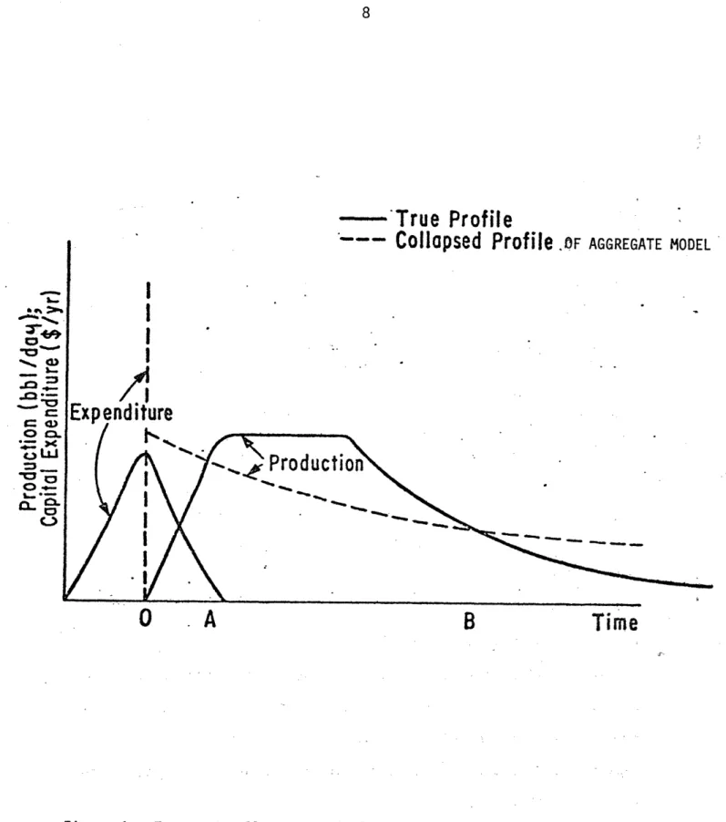
Whichever method we use, application of a single depletion rate to a

reserve estimate -- to obtain a production profile -- is a strong

simplification, as Figure 1 shows. In the graph, the solid line labeled "Production" shows a typical production profile for a field; the area under the curve is the total proved reserves, R. The dashed "Production"

line is our simplified version of oil exploitation where production jumps

3

immediately3 _{to an initial (and presumed peak) capacity Qp and declines}

4

at a constant percentage rate thereafter. Once again, the area under the curve is R, so that:

T

C _ e-at

R = Qp e atdt . (5) v

t=O

As T *, R Qp/a; or in the limit, a = Qp/R. The question for v

analysis then is: what is the value of the depletion rate, a (and

therefore of Qp), that is appropriate for new additions to reserves? v

Once a is determined it is a simple step to forecasts of supply, as then

3_{The equating of capacity with production is realistic for}

price-takers, but for the cartel it assumes that those nations are not forced to hold excess capacity in order to help support the price.

4_{Later we discuss a method of lags in}

this buildup to Qp which gives us a closer approximation to the actual profile.

I - -8

---- 'True

Profile

I

I

I

Expenditure and Production Profiles

0

. A

B

Time

______ ___I .---II L- L -

--I-.I%

I----4.-

Qt = aRt. The remaining issue is the lag between the point when proved reserves are "booked" and the point when the new capacity Qp is on line. In a mature producing area the lag from the former to the latter is short, but not in a new province, such as Mexico's Reforma. But data on lag profiles is difficult to obtain. Thus, as a first approximation, for onshore areas we assume a two-year development lag in which new proved

reserves are producing at 40 percent of their peak capacity in the first year and the remaining 60 percent is brought on in the second year. For offshore areas we assume a four-year development lag which brings on the additional capacity in 25 percent increments in each of the four years.

The "Expenditure" lines on the graph in Figure 1 illustrate our required assumption as to capital investment. The solid "Expenditure"

line represents the usual path of expenditures to produce the true (solid line) "Production" path. But in order to conform to our model hypothesis that Qp begins immediately, we collapse all capital expenditures to the same point in time as the dashed "Expenditure" line on the graph. The

implications of this assumption will be discussed in our net present value analysis later.

1.3 Estimation of Additional Productive apacity

As a first approximation, capacity plans can be calculated on the assumption that new additions to proved reserves will be depleted at the

same rate as existing fields. Under the assumption of a uniform policy regarding depletion, the depletion rate for an area can be calculated as a simple arithmetic average:

1975

a

a 3

-

t=1973

---J -

-10

where 1973-75 is again taken as a reasonable base period for estimation. Then for any new addition to proved reserves in year t, the new installed capacity is:

aQpt = aaR_{AQ~aA R t} · (7)₍₇₎

Assuming no excess capacity is installed, production from Rt begins at the level Qt = Qpt and declines at "a" percent per year. But the

calculation of Rt used in (7) is no simple task. Using the method of Equation (1) requires data on the changes in proved reserves. Usually these data are too inaccurate for use, thus the results are untenable and we do not report them here. An alternative is to take the difference in production between year t and (t - j) and add it to the estimated loss of productive capacity (cumulative decline) from j to t. This would be a direct calculation of Qpt in (7). This requires the accurate

measurement of the decline rate, which we do not have except in the U.S. Moreover, wherever there is irregular fluctuation in output, or any

appreciable amount of excess capacity, the method cannot be used at all, since change in output is no indication of change in capacity.

A second method is the following. From published data we can calculate the average well productivity of an area as:

average flow rate per well = Qt/Wt (8)

where Wt is the number of producing oil wells in a given area in year t.

We can also calculate the number of newly drilled wells, Wt, and the rig-time needed to drill a producing oil well as:

rig-time per well = aWt/RYt (9)

Using 1975 as our general base year, we can estimate the new capacity in an area for period t from our forecast of development rig-time in period t as:

aW75 Q7 5

Qt = RYt (R75) 75 (10)

We term this method the "Average Flow Rate Method." Equation (10) thus gives us an alternative to (7) for an estimate of Qt.

However, this average flow rate method tends to understate capacity increments to the extent that new wells are always drilled with better knowledge of the reservoirs than old wells, and to overstate increments because one would expect lower well productivities because of well

interference and decline, and as lower-quality strata and reservoirs are developed. Perhaps even more important, an average for any area may

include low-output fields where there is little drilling because it is not worthwhile. Thus, to the maximum extent possible, one should

segregate Rt,a and therefore Qt by separate fields, or areas.

We approximate this desired segregation by our third method of estimating capacity changes, the "Weighted Average Flow Rate Method," where we substitute a field-weighted flow rate per well for the average flow rate used in Equation (10) above. Our estimate of the weighted

average flow rate per well for each area is calculated as follows:

m Q

estimated weighted average flow rate =

2

where m is the number of major fields (a major field is defined as one which accounts for at least 3 percent of the country's total production),

Qi is the production of major field i, QM is the total production of all major fields, i.e.,

m

QM Qi' and W_i is the number of producing wells in major field i. V

i=1

--I-12

Thus QMM is our weighting factor and

£

=

i=l (M

We can substitute from (11) into (10) to get:

aW75 m Qi Qi

aQt = RYt E ( ( ) ( )) (12)

75 i=1 Q i

where (10) is the (simple arithmetic) average flow rate method and (12) is the weighted average flow rate method. Depending on which of these methods is chosen, capacity in area i is thus: Qt + aQt where Qt is

corrected for the decline effect from Qt-l' Some independent estimates of capacity are available for recent years for OPEC countries and can thus be used as a crosscheck. A comparison of the average and weighted

average methods follows.

1.4 Historical Production-Reserve Ratio

The observed production-reserve ratio for any country is based on an aggregate of many fields. Hence, for reasons already examined, a simple division of national production by national reserves may be seriously misleading. A good example is Table 1, showing Abu Dhabi. Total

national production was 1.7 percent of proved-plus-probable reserves. But the bulk of those "reserves" is still undeveloped; the true working inventory is being drawn down much faster. The simple quotient Q/R = .08 gives equal weight to every barrel of developed reserves. But our true objective is to give equal weight to every barrel produced. If we want to estimate how much Abu Dhabi is capable of producing next year, the Bu Hasa field (156 million barrels) is approximately twice as important as Zakum (82 million).

____ I.----·-·-nBI-LII

-Accordingly, we weight the production-reserve ratio for each field by its share of total country production (as per equation (11)). This

calculation is shown in _{Table 1. Use of the weighted average lets us} escape from some of the ill effects of poorly estimated reserves as well. Since it is a better predictor of future production, it yields more accurate cost data, which depend on our estimated production profile

(Figure 1). We have, of course, a minor sampling problem since we are using the average of the listed fields as a proxy for the whole country. However, the finite population multiplier is a powerful ally; since we have accounted for 77 percent of the national total of production

(394/512), the error cannot be great.

The weighted mean is a more reliable indicator of cost and it forces us to look at the several fields to see their capabilities for

expansion. An abnormally low (Qi/Ri) may indicate overstated proved reserves in that more investment will be needed to drain the number of indicated barrels. Or it may signal an underdeveloped field.

A little reflection on the meaning of a "field" as a collection of adjacent or overlapping reservoirs, and the usual development pattern of going from one to another pool or horizon, will show that the correction among fields must, to at least a modest degree, also apply within

fields. Hence, even the weighted mean must involve some understatement of the true depletion rate.

It is likely that outside the United States and Canada, reserves are overstated and therefore decline rates understated. This is not because of errors of optimism, but because undeveloped reservoirs in known fields

tend to be counted in.

Beginning with 1978, IPE no longer presents estimates of reserves in the largest fields. It will be necessary to close the gap in the sources.

I . .

-14

Table_ _ Weighted Mean Depletion Rate, Abu Dhabi, 1975 (millions of barrels) Major Field, Discovery Date Asab, 1965 Bu Hasa, 1962 Mubarras, 1971 Um Shaif, 1958 Zakum, 1964 Subtotal

Total Abu Dhabi Fields

Prod ucti on Q 90 156 7 59 82 394 512 Reserves R 500 1,289 150 1,706 1,314 4,959 29,500

Unweighted Mean, total Abu Dhabi = 1.7 percent Unweighted Mean, Large Fields only = 8.0 percent Weighted Mean, Large Fields only =

[Qi(Qi/Ri)]/'QM = 42.6/394 = 10.8 percent

l ~ M

Sources: Unweighted Mean, OGJ; others, IPE.

Q2/R 16.2 18.9 0.3 2.1 5.1 42.6 Q/R .180 .121 .047 .035 .062 .080 .017 _ ___ _U_ __I_ _ _ U)_ I__^____I_____ I _ _ _1___1___1

1.5 Optimal Depletion Rate

The value of "a" observed in historical data, and calculated by Equation (6), is the result of a particular set of past conditions of costs, prices, and taxes. It may or may not be an appropriate guide to future behavior under different conditions, and therefore we should like to be able to calculate this parameter more exactly. In theory, we can do this by assuming profit-maximizing behavior on the part of oil

operators, and solving for the optimal depletion rate, a*, based on estimates of cost per barrel and future price.

First, it is assumed that the profile of capital expenditures shown in the graph of Figure 1 can be collapsed to a single-period outlay I. Data on operating costs are rather sketchy; fortunately the bulk of costs is usually capital outlay, and this can be approximated by an adjustment to I, as shown below. We also assume that the capital coefficient, I/Qp is a constant; later we consider the effects of a capital coefficient which is higher at higher depletion rates.

By our simplified model of depletion, annual production is

Qt Qpe -at. Let I(Qp) be the capital expenditures required (as a rising function of the level of initial peak production) to establish production level Qp. Given a constant expected future oil price, P, and discount rate, r, the net present value of a block of reserves becomes:

T

NPV =[PQp e-(a r)tdt]- I (13) v

t=O

Letting T *+ we may write (13) as:

PQp

NPV a+ r - I (13a)

·

---16

Qp is _{the choice variable and to maximize NPV in (13a) we set}

a(NPV)/aQp = O, _{which gives the necessary first-order condition for}

maximizing the value of the reserves. That first-order condition can then be solved for the optimal decline rate, a*, as:

1/2

a* = - r (14)

3Q

where we now explicitly consider price per barrel, P, and marginal

capital costs, aI/aQ. Thus the optimal depletion rate is a function of the capital coefficient (or, more properly, its reciprocal), the oil price, and the discount rate. If we consider the project as a whole,

then aI/aQ = I/Q.

With no constraints on the decline rate, we can now solve for the optimal production capacity in year t as:

Qt = (a*)(Rt). (15)

In _{any given reservoir, production must some day cease because the} total variable costs tend to be constant per well or grouping of wells and therefore variables costs per unit must in time rise with declining output to where they exceed the value of the output. Hence the depletion rate a = Qt/Rt must increase; in its last year, Qt = Rt and the rate is unity. For a group of reservoirs the observed a is biased upward; hence if _{the decline rate approximates the true depletion rate, the observed a} tends to overstate it. The longer the life of the field, the less

important the bias; generally speaking, it becomes negligible for reservoirs operating over 25 years ([1]), Ch. 2, Appendix).

Before proceeding to estimate values of I/Qp and a*, it is worthwhile to question the accuracy of the simplified or "collapsed" model of oil

__ __1_111 _____ ________________I_ _·CI __I

exploitation shown in Figure 1. We have reduced a complex process to only three parameters-total proved reserves, total (or incremental) investment, and peak or initial output--and we need to make sure that this model yields a reasonable approximation to reality in view of the wide variations in _{production profiles among fields, and the dependence} of the results on the discount rate assumed.

We can get a rough check on this issue by comparing the average per-barrel cost of oil as calculated by our "collapsed" model against actual data on expenditure and production profiles for the North Sea. Referring to Figure 1, we can define an oil price, C, which would meet the condition T T NPV = Et e rtd t -( CQt e- rtd t = (16) t=O t=O

where Et is investment expenditures in period t. This C is the supply price of oil from the reserves illustrated in Figure 1. Or, more

usefully for our purposes, C may be referred to as the average cost per barrel of oil from a new project in the area shown. We are able to calculate the "true" value of average per-barrel cost from

Wood-MacKenzie's detailed data for seventeen North Sea fields.

Similarly, by setting NPV = 0 in _{Equation (13), inserting equivalent} values of the "collapsed" parameters, and solving for P, we can calc late a comparable set of figures for the simplified model. When we estimate C = o + _a

1P using the values of C and P thus calculated, the results are

.. .I

--18

Table 2. North Sea Cost Estimation Discount Rate, r (O al R2 SE CV 10 -.028 (-0.19) 0.972 (16.5) .95 .177 .078 12 -.033 (-0.18) 0.989 (14.4) .93 .224 .089 15 -.046 (-0.18) 1.013 (12.0) .91 .310 .107 20 -.055 (-0.13) 1.067 ( 9.5) .86 .487 .133 (Numbers in parentheses are t-statistics, SE = standard error of

regression, CV = coefficient of variation. Source of data: Wood,

MacKenzie and Company, Section 2 of the North Sea Service, February 1976.) For example, in Table 2, with a 12 percent discount rate, the

"collapsed" unit cost, C, is a little higher on the average than the true cost: to get from "collapsed" to true, one multiplies collapsed by 0.989 and subtracts 3.3 cents. Thus estimated, the calculated cost differs by

less than 9 percent of the true cost in two-thirds of all cases.

Whatever the discount rate, however, the collapsed cost is a reasonable approximation to the true cost. But this good fit depends critically oni the strict definition of reserves as "planned cumulative output from planned facilities," as discussed above.

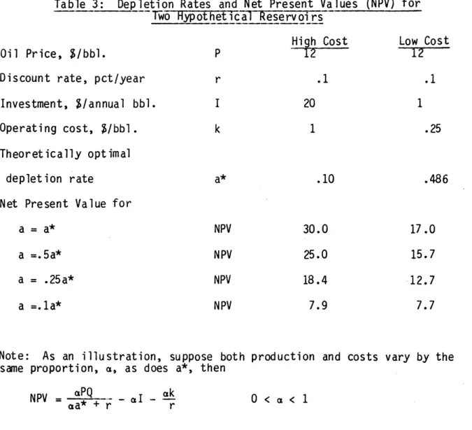
Two very general qualifications must be made at this point, First, Bradley [7] has pointed out that the marginal cost increases essentially as the square of the depletion rate. Therefore, in the neighborhoo of optimal depletion much is saved by slightly lower rates of output. The reduction in net present value is disproportionately small compared with the reduction in the rate of output. In Table 3 below we consider two hypothetical projects: one high-cost deposit with $7,300 per barrel of initial daily output and operating cost of 1 per barrel; and one very

low cost deposit, with $365 per initial daily barrel and 25 cents per barrel operating cost. The high cost deposit has a net present value of $30 at the optimal depletion rate, of 25 at 50 percent of the optimal rate, and 18.40 at one-fourth of optimal. The decline of net present value of the low cost deposit is even more gradual.5

This relation of NPV to depletion should be considered with the increasing investment requirements per unit of output as one goes to higher depletion rates, discussed below, and with the pervasive

uncertainty regarding the characteristics of any reservoir. Since the correct discount rate and cash flow distributions are very difficult to

ascertain, this trade-off of NPV for considerably lower investment and output might be an acceptable proxy for risk and risk-reduction.

Particularly in a newly developing area, even with no other constraints, we might expect to see the actual depletion rate be a minor fraction of the theoretical optimum. Given high risk, the best investment pattern might be to sacrifice more than half the net present value in order to reduce the investment and risk exposure by 90 percent, as shown in the example in Table 3.

Because of these limitations, and particularly in view of the "Bradley effect" in proxying uncertainty, the usefulness of our

theoretically calculated a* as a guide to normative investment policy is much reduced. It serves mostly to open questions. That is, if the

operator is without cartel inhibitions, if his reserves are correctly stated, and if we also have some confidence in the cost estimates, we can

5_{Parenthetically, the somewhat lower net present value of the lower}

cost deposit is achieved with an investment only one-twentieth as great, and an operating cost only one-fourth as great.

20

Table 3: Depletion Rates and Net Present Values (NPV) for Hypothet- -ical

Reservoirs

Oil Price, $/bbl.

Discount rate, pct/year Investment, $/annual bbl. Operating cost, $/bbl. P r High Cost .1 20 I k 1 Theoretically optimal depletion rate .10

Net Present Value for

a = a* a =.5a* a = .25a* a =.la* NPV NPV NPV NPV 30.0 25.0 18.4 7.9

Note: As an illustration, suppose both same proportion, a, as does a*, then

NPV = aPQ -aI - ak

aa* + r r

production and costs vary by the

0<a< 1

aNPV PQr k

(aa* + r) r

Thus, in choosing a, the higher are I and k, the worse the trade-off; the higher are a and a*, the better; r works both ways.

Low Cost 12 .1 1 .25 .486 17.0 15.7 12.7 7.7 ___il__ll__g__r_____lll --

·C---·ll_-ask why the depletion rate is, say, less than 50 percent of theoretical optimal, and what kind of nonlinearities, or risks thereof, are being allowed for.

In both of the examples in Table 3, the discount rate has been taken as 10 percent. Higher or lower rates would not substantially change the picture in these examples. However, some reflection on them is

worthwhile if in our modeling work we try to capture greater risk.

In general, a higher interest rate will have two opposing effects on the optimum depletion rate. Because it makes future use less attractive compared to present, it will tend to speed up the rate of depletion. But because it makes production in this capital-intensive industry more costly today, it tends to slow down the depletion rate. The net result

is not predictable, and a higher interest rate may on balance result in a slower depletion rate. More often, however, it will likely speed up depletion.

A higher discount rate is often used as a proxy for greater risk, and this is proper when it implies a higher yield is necessary before an

investment is to be undertaken. But particularly with the low cost deposit, it may be irrational for an operator facing a high degree of political risk or moral hazard to allow for it by using a higher discount rate which might lead him to speed up the rate of extraction. Instead, a risk-avoiding profit maximizer may limit sharply the rate of extraction, thereby avoiding the great bulk of the potential loss (of investment) at only a very modest penalty in net present value. For now we cannot make a definitive statement; this problem will be explained formally in a future paper.

22

As Table 3 suggests, and as shown by differentiating net present value with respect to the percentage reduction in the depletion rate, the higher the level of costs, the stronger the reduction in net present value for any given reduction of the depletion rate. Hence, given high costs, perhaps in a well-established area, the reduction in depletion rate will not be nearly as strong as in a low cost and usually newer area.

1.6 Analysis of Capital Costs

1.6.1 Constant Capital Coefficients

Unfortunately, outside the North Sea, we do not have anything

remotely resembling these detailed investment data. Capital coefficients for differing producing areas can be estimated only very roughly from historical data. Operating cost data are even more scarce. Indeed, the lack of cost data is at present as great a gap as the lack of reserve data.

In addition to this bias, there is also year-to-year inaccuracy caused by the lumpy nature of much development investment, especially in lease equipment and loading facilities. The amount invested per unit of additional daily output will be exaggerated in a year with much work in process and little completed. Conversely, investment is understated in the year facilities are completed, and the facilities may begin operating with little new money being spent.

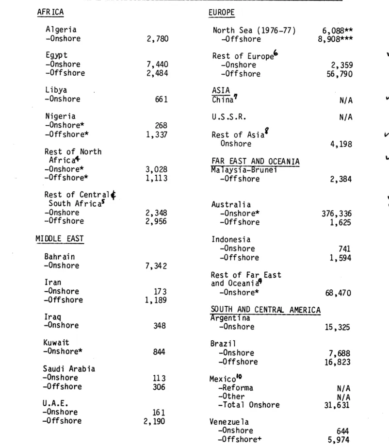
We have estimated investment requirements per additional daily barrel. They are presented in Table 4 and are in concept "average cost at the margin." That is, they are an estimate of what was required, in a recent time period, to install an additional barrel of daily capacity. They do not allow for the feedback effect of additional production from new wells which would cause the capacity of existing wells to decrease.

____I

-Total investment is a product: rig-years multiplied by the average cost per rig-year. The latter has been derived from U.S. data. It is a simplified version of the estimates to appear in another working

paper.6 It includes expenditures on drilling, lease equipment,

secondary oil recovery, and overhead. All drilling time is included, which tends to overstate expenditures because some is exploratory and some result in gas wells. Injection wells are of course included. Onshore and offshore have been estimated separately.

New oil production capacity is the product of new oil well

completions in the area multiplied by the weighted average flow rate per well. Then dividing total investment as determined above by this new capacity estimate yields the results in Table 4.

Offshore production is usually, but not necessarily, more expensive since higher cost per well may be more than offset by higher productivity.

The years included were 1974-76, but the estimates have all been transformed into 1978 dollars by the use of the IPAA cost index. Some of the estimates are unreliable and implausible because there are too few observations. For example, the Kuwait number is improbably high (6 well completions in three years), as is "rest of Europe-offshore" (2

completions) and "Far East and Oceania" (3 completions). "Australia onshore" might serve as a horrible example: 10.5 rig-years, with one oil well completion, and an average flow rate of 15 barrels daily, yields a coefficient over $300,000!

The principal weakness of this kind of estimate is, of course, the averaging-together of very different areas and formations, with

24

corresponding differences in cost. In any given area, if it is large enough to be worth the additional study, we can hope to do better, particularly if oil companies can furnish us more detailed information. For example, we might try to observe which particular fields were

expanded in a given year, and thereby improve our estimate of new

capacity (the denominator). Or we might be able to allow for unusually heavy costs in a pressure maintenance program, thus improving our

numerator. For lack of such data, the Iran onshore is surely too low. The Saudi Arabia onshore is also too low, for lack of allowance for the Ghawar waterflood project. However, the recent highly publicized

estimates by the U.S. Senate Foreign Relations Sub-Committee have

exaggerated the costs of that project by a factor somewhere between five and eight. It appears to be due to simple miscopying, whereby the total outlay, not only on the water injection scheme but also on gas

processing, liquid separation, gas pipelines and oil pipelines, etc. were all assigned to the water injection project.

Capital coefficient estimates can be used to check on the calculation of a*. As an example, take a North Sea field where

investment per peak daily barrel is calculated (from Wood-Mackenzie data) to be $7,300. We will take r as 10 percent.7 The oil price is assumed

7_{During 1975-76, dollar-denominated Eurobonds had a 9 percent yield,} which we consider as the prime business-risk rate on long-term financing. We

add 1 percent, which is the average premium above the LIBOR (London Inter-Bank Offered Rate) on secured financing for the North Sea development projects.

Perhaps a better inflation allowance would start from the fact that the Sterling LIBOR was generally 4 percentage points above the dollar LIBOR in

1975-76 (9.5 and 5.5 percent respectively) before the sterling slide in late 1976. An interesting confirmation of our 10 percent discount rate is in the LASMO-SCOT "package" rate, in late 1976, which can be shown to approximate 14 percent in Sterling (see the LASMO-SCOT Prospectus, February 1976).

Table 4. Investment Of Capacity, Various AFRICA Algeria -Onshore 2,780 Egypt -Onshore -Offshore 7,440 2,484 Libya -Onshore 661

Requirement per Additional Dai Countries, 1974-1976 (in 1978 ly Barrel dollars) EUROPE North Sea (1976-77) -Offshore Rest of Europe" -Onshore -Offshore ASIA Chinaq 6,088** 8,908*** 2,359 56,790 N/A Nigeria -Onshore* -Offshore* Rest of North Afric a4 -Onshore* -Offshore* Rest of Central¢ South Africas -Onshore -Offshore 268 1,337 3,028 1,113 2,348 2,956 MIDDLE EAST Bahrain -Onshore _7,342 Iran -Onshore -Offshore 173 1,189 Iraq -Onshore 348 Kuwait -Onshore* Saudi Arabia -Onshore -Offshore U.A.E. -Onshore -Offshore 844 113 306 161 2,190 U . .S.R. Rest of Asiat Onshore

FAR EAST AND OCEANIA Ma laysia-Brunei -Offshore Australi a -Onshore* -Offshore Indonesia -Onshore -Offshore Rest of Far East and Oceaniaq

-Onshore*

SOUTH AND CENTRAL AMERICA Argenthorna -Onshore Brazil -Onshore -Offshore MexicoI° -Reforma -Other -Total Onshore Venezuela -Onshore -Offshore+ V N/A V 4,198 V 2,384 V v 376,336 1,625 741 1,594 V 68,470 15,325 7,688 16,823 N/A N/A 31,631 644 5,974 I I _ ____ __ _ __ _ _

26 Table 4 (continued) Rest of South Central America -Onshore 1,447 -Offshore _3,173 NORTH AMERICA Canada U.S.A. (lower 48) Alaska Notes to Table 4

*Indicates weighted average omits one or more of years due to too few reported rigyears or well completions these years.

**Excludes costs of transportation to shore. ***Includes costs of transportation to shore. +Lake Maracaibo.

N/A indicates not available.

Numbered footnotes are in Appendix I.

___ _____1_____1___1___II_

-to be 12.50 per barrel, and initial operating cost (at peak production) is $.95 per barrel,8 i.e., 347 per year over the life of the field. Assuming the typical North Sea field's 20-year life, and a 10 percent discount rate (estimated as discussed above), a stream of outlays or receipts of 347 per year is worth approximately (347)(8.65) = 3,000. Investment plus operating cost now equate to a capital sum of $7,300 +

$3,000 = $10,300. Then:

* /365()12.50) (.10)

a* --- - 10 = .110 (17)

In fact, outside of Auk and Argyll, observed North Sea Qp/R ratios (which are an approximation of a*) are about 9 percent. We will see shortly why they should be expected to be a bit lower than optimal.

As another example, we may take the hypothetical field "discovered" by Conoco on the Georges Bank (Oil and Gas Journal, July 19, 1976, p. 60). It contains 200 million barrels, to be drained in 15-20 years (say, 17.5) and requires an investment of 397 million. We assume operating costs will be slightly lower than Montrose and Heather (slightly smaller fields) in the North Sea, i.e., 25 million annually, over a 17.5 year period hence with a present value of 207 million; total investment is

then $604 million. Initial output is 60 thousand barrels per day, hence the total capital coefficient is $10,066 per daily barrel.

Conoco assumes P = 14 per barrel, and hence our estimated a* 12.5 percent. Conoco's estimate is 10.95 percent.

8_{Wood-MacKenzie report, October 1976, Section Two, Table 1, average}

for all proved fields.

28

Another comparison is possible, using a paper prepared at the U.S.

Geological Survey ( ). The authors hypothesize a reservoir with a given V quantity of producible gas, reservoir pressure, price-cost parameters,

and four possible rates of water encroachment. The operator's decision on number of wells determines the initial Qp, the ratio Qp/R, the

production profile over time, and the NPV of the deposit. Since price, operating costs, taxes, and the capital coefficient can be approximated from their data, and the interest rate is given, we can calculate a* =

.135. In fact, the ratio which they calculate would maximize NPV is in the range between .157 and .173. (Although ultimate recovery is

sensitive to the rate of withdrawal, there is no well interference, and initial withdrawal is explicitly stated as strictly proportional to the number of wells drilled.)

Finally, there is a hypothetical Gulf of Alaska field [11, see also Appendix II], where, on the data given, a* would range from 9.2 to 12.6 percent assuming lower costs, or from 6.4 to 10.4 percent assuming higher costs. In both cases, the lowest depletion rate is for a 20 percent

discount rate, the highest depletion rate for a 10 percent discount

rate. The actual depletion rate, i.e., peak-year production to total, is 11.7 percent. However, this is not the result of any optimizing

calculation, but only a modal or "typical" plan.

It should not be supposed that depletion or decline rates above 50 percent are bizarre or impossible. It all depends on the particular reservoir. Miller and Dyes [9] analyzed optimum development in a hypothetical reservoir where the operator was free to, and did, seek maximum net worth. The reservoir contained ten million barrels in place. With a solution gas drive, 1.8 million barrels would be

recovered; under a complete water drive, 4.1 million. In each case, present value changes very little in the neighborhood of the optimum

number of wells, e.g., for solution gas drive it decreases approximately 14 percent for two wells, as compared with four wells. Decline rates were respectively 66 percent and 78 percent.

1.6.2 Variable Capital Coefficients. So far, it would appear that a* gives values not too far out of line with reality. But the three validation examples have been very high-cost areas. In low-cost areas, we must expect depletion rates to be generally below computed a*. This is to be expected for various reasons:

1. Published "reserves" may greatly exceed true proved reserves, i.e., planned cumulative output through existing installations, even when labeled "proved."

2. Risk avoidance because of the "Bradley effect" (discussed above). 3. The operator may be inhibited by a fear of spoiling the market, or by an understanding to keep output down in order to maintain prices. This is obviously the case with the core cartel countries. 4. The most important reason is that marginal investment

requirements per barrel of additional capacity, or operating costs per additional barrel, may go considerably above the average as calculated in Table 4.

At low depletion rates, investment requirements may decline as indivisibilities are spread thinner: access roads, supply dumps, etc. But at a fairly early stage these scale economies tend to become

insignificant. Thereafter, there may be an interval, short or long, over which investment and operating cost requirements are relatively flat for the whole hydrodynamic system is involved: the oil in place (including

30

dissolved gas), any associated gas, and water. The volume and pressure of the hydrocarbon may be a minor or very tiny fraction of the whole. But usually, past some point, the higher the total output, the lower the output per well. Hence, there is a margin where the output gained by drilling a well declines, perhaps sharply. And at some farther point the increase in output per additional well may become extremely nonlinear, even negative. Too high a rate of output may cause gas to come out of

solution, or water to break through to the well bore ahead of the oil, in which case output per well may be considerably decreased or cease

altogether, and ultimate recovery may be much reduced. Thus the cost of an increment from Qn to Qn+1 may be much greater than from Qn-1 to Qn'

In the United States, where reserves are estimated strictly on a very large sample of reservoirs, since 1972 there have been no restrictions on output. Despite incentives to speed recovery, the ratio of production to proved reserves has been very stable in the neighborhood of 11.8

percent. It is expected to remain there, and production out of proved reserves to decline at that rate ((5), p. 214). Smaller areas are as low as 9.0 (California, San Joaquin basin) or as high as 24.6 percent (Texas, District 5)(5), (Table I).

In a mature producing area, the mean depletion rate must exceed the ratio Qp/R. _{(At the extreme, imagine a reservoir which will close down a} year from today. The ratio today is then unity.) In an area where

reserves are actually declining, the bias is more pronounced. During the last years of near-universal stability of reserves in the United States, 1959-61, the mean percentage was respectively 7.82, 7.82, and 7.86 [6, Table II]. A new reservoir would have had a lower Qp/R. In more recent years, new reservoirs may not have had any higher ratios.

11 -- -__I___.1_ -.1______~~ I

The United States also provides us with a good example of a very large recently opened field, Prudhoe Bay in Alaska. In early 1980, its optimal capacity was put at 1.5 million barrels daily, and reserves of

8435 million barrels [11]. Thus the optimal 1980 depletion rate was 6.7 percent. In a developed field, the traditional suitable rate is 6.7 percent (i.e., reserves 15 times output). If, therefore, the U.S.

average is nearly twice as high, this is a bias of observation. We should expect new fields in California (San Jaoquin) to be well below 9 percent; in Texas (District 5) well below 25 percent. This gives us an idea of the limits imposed by reservoir behavior, which raise (aI/aQ), hence constrain a*. Therefore we might reckon that in most fields the ceiling to depletion rates must be in the low teens.

To make I, the investment, an increasing function of Qp/R, James L. Smith has devised the following approach. We specify the reservoir

investment function as:

I = KacR (18)

with K the proportionality constant and (epsilon) the elasticity of

investment with respect to the depletion rate. Since aR = Qp, varying

e in a R will vary the investment as a function of chosen output (i.e., the depletion rate). The constant K merely translates planned initial output into dollar requirements. Thus e = 1 implies constant (linear) costs; > 1 implies increasing costs, etc.

The equivalent of Equation (13) is: P Q

NPV= a P - Ka£R (19)

and the optimal initial depletion rate can be expressed in the following relation:

---32

a* r=

r

EK(a*)-1

Note that equation (14) is just a special case of (20), where e = 1 and

therefore K = I/Qp. The a* in Equation (14) implied that well

productivity had not yet entered the phase of diminishing returns. But Equation (20) now lets us obtain a marginal cost which allows for the increasing costs imposed by well interference or by any other cause of diminishing returns; and to derive an optimal initial producing rate accordingly.

With an estimate of £, we have all the parameters needed to solve for

a*, with the exception of the constant K. By Equation (18) we can state K as a function of I/Qp and a, and we have the historical value of the

capital coefficient, and the depletion rate , which are proxies

capital coefficient, I/QpI and the depletion rate , which are proxies

for the true values. Thus:

K = Qp)a :I (18a)

With K as estimated by (18a), we can solve Equation (20) (we use an iterative algorithm that permits a numerical approximation) for the optimal future depletion rate a*.

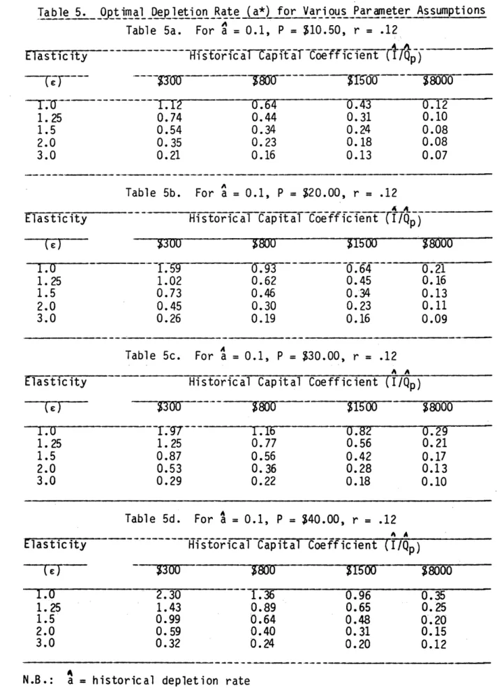
Table 5 shows some of the results, assuming the historical depletion

rate was 0.1, P = 10.50, and r = .12. The reason why we need this

procedure is not far to seek. The range of observed capital coefficients is enormous. The top line of Table 5, which puts the interference effect to zero (i.e., £ = 1), would indicate that with particularly low capital

requirements (300 per initial daily barrel) the oil should be brought out in less than a year. But: (1) it is probably physically impossible

Table 5. Optimal Depletion Rate (a*) for Various Parameter Assumptions Table 5a. For a = 0.1, P = $10.50, r = .12

Elasticity f torfCa-TTpitaT Coeficient (Ip)

$300 g8Uu 1.12 0.74 0.54 0.35 0.21 U .64 0.44 0.34 0.23 0.16

-I---rr--~- -- -- ·- IrPI--- - -I__~~

g1buu ---0.43 0.31 0.24 0.18 0.13 Table 5b. For a= 0.1, P = 20.00, r = .12 Elasticity Historical Capital Coefficient

(/P)

WJUU b15oU 1 . 0 - -- --- -. 64 0.21 1.25 1.02 0.62 0.45 0.16 1.5 0.73 0.46 0.34 0.13 2.0 0.45 0.30 0.23 0.11 3.0 0.26 0.19 0.16 0.09 A Table 5c. For a = 0.1, P = $30.00, r = .12 A

Elasticity Historical Capital Coefficient (I/Qp)

(~) ~~ -300 __500- :800 8000 1.U o - 16 .7. 0.82 0.29 1.25 1.25 0.77 0.56 0.21 1.5 0.87 0.56 0.42 0.17 2.0 0.53 0. 36 0.28 0.13 3.0 0.29 0.22 0.18 0.10 Table 5d. For a = 0.1, P = $40.00, r = .12

Elasticity --- Hi a--C-- i c ient ( I/Qp)

(TV7 c-8ssr- ) -- 8-- -- % 1500 -$0 $8000 1.0 1.25 1.5 2.0 3.0 2.30 1.43 0.99 0.59 0.32 1.36 0.89 0.64 0.40 0.24 0.96 0.65 0.48 0.31 0.20 0.35 0. 25 0.20 0.15 0.12

N.B.: a = historical depletion rate

P = price r = discount rate 1.0 1.25 1.5 2.0 3.0 ~8uu 0.12 0.10 0.08 0.08 0.07 4 I-~80UU b, I' V U, I - - - -F-~~~_

-I--

-- --- --- "~

34

to drill and complete the well and equipment so quickly; (2) The

draw-down could not be sustained; the attempt would damage the reservoir and lose reserves; (3) The attempt to install so much capacity so quickly

A A

would drive the value of K far above the historical value of I/Q; and, (4) So high a rate of initial output would reduce output per well, again raising the value of K above past observed values.

Hence the use of e and the algorithm of Table 5 is to isolate cases where neither (1) nor (2) governs, and to put at least some subjective value on the effect of (3) or (4) or both.

A final qualification: an expectation of higher prices would, ceteris paribus, justify delaying output and thus lower a*. This is a problem in optimal control theory, and we intend to work out the

functional relation in a later paper. 1.7 An Example -- Mexico Reforma

The aggregated method herein described, with national entities as building blocks, treats as one reservoir what may be a collection of hundreds. Small countries may be left that way. But larger ones must, as soon as possible, be divided into rational subgroups. In every case, we divide between onshore and offshore. We can illustrate our method

using the important new Reforma area of Mexico.9 In this region, the new reserves-proved, probable and ultimate--have all been added since 1972, and therefore we treat the area separately from the rest of Mexico. To

9_{The Mexican authorities use a definition of proved reserves which} is very close to the strict API concept: "reserves which are expected to be produced by existing wells through primary and secondary recovery;" from Prospectus, Mexico External Bonds Due 1983 p. 17, (September 1976).- At a later stage, the definition may have been relaxed; but our data relate to the earlier unambiguous period.

apply to the newly developing areas the coefficients derived from areas 50 to 75 years old would have been right only by chance.

In Table 6, we set out the number of development rigs operating in the Reforma area. We assume, provisionally, that the number stays constant at the level reached in March 1979, in order to examine the

consequences. In column 2, we show the number of wells operating, and in column 3, the output (including a small amount of natural gas liquids). Diminishing returns are shown by the bt coefficient, and amount to 8 percent per year by 1985. Were we to use a higher estimate of ultimate

reserves than 55 billion, the decline would be less. The coefficient is set at unity for 1976, on the theory that the area was too little

developed until that time to make it worth calculating, and to start the simulation at 1977.

By comparing the increase in the number of wells with the number of rigs, one sees the number of wells dug per rig year. For 1973-76

inclusive the average (or strictly speaking the coefficient in a

regression) was only .642 wells per rig year, or 18.75 months to drill a well of 14,000 feet. This is an unusually slow rate, and should perhaps be ascribed to the problems of opening a new area.

Had we no other information, we should have overridden this drilling rate on the basis of information from other sources. Fortunately, we had a far better means of correction, from a Pemex document, which gave the complete drilling plan for 1978. It showed an average of 5.53 rig months per well which we rounded up to 6.0 rig months. The same document showed an average allowance of two months for moving a rig from one site to the next, for a total of 8.0 rig months per well, or 1.5 wells per rig-year. We lowered to 1.2 on the theory of one-fifth slippage as the number of

36

Table 6. Calculation of Production in Reforma Fields, Mexico

Assumptions: Proved Reserves are 55 BB end-1978; initial output per well is 5500 bpd.

Development Wells

Year Rigs Operating

19 / 1974 1975 1976 1977 1978 1979 1980 1981 1982 1983 1984 1985 (4) (5) bt Forecast

Coeff icient Output

(tbd) 45 44 44 45.4 58.5 90o 90 90 90 90 90 90 109 142 250 358 466 574 682 790 898 1.0 .813 587 760 1379 1936 2465 2944 3369 3731 4023 a90 rigs in March 1979.

bFirst six months average, OGJ, Dec. 26, 1977. Source: Adelman and Owsley [3].

- -(6) Actual Output (tbd) U 113 288 432 600 865 1117 CrCTIU - ----· -- -'---L--- --- --- ·--- --- j+--- ---- ·-- __ --- ----2/

rigs built up so sharply. This number was applied to column 1, to obtain annual additions to the total shown in column 2. Output is estimated by starting with 5531 barrels daily per well in 1979, then declining to 4480 with the bt coefficient, as explained.

Early in 1978 it _{was announced that a figure of 2.25 million barrels} daily for Mexico (hence about 1.81 for Reforma) would be attained in 1980, not 1982. This makes our simulation too high by 130 tbd, about 7 percent. On the other hand the chief of development for Pemex said, in May 1978, that production could be increased by 500 tbd throughout the

1980s. This confirms that the buildup is too high by 100 tbd and then by 60 tbd in 1979 and 1980, but then decreases too fast; the bt coefficient is dropping too fast.

If this was correct, the rig buildup in Reforma should be over. The current ceiling for Reforma production is 2.16 (or 2.5 for all Mexico). Even with 90 rigs, a target reached in early 1981, it will soon be much surpassed. Hence we can watch the total of drilling rigs operating there (and make an estimate of development rigs) as an indication of investment and production planning. If the rig total is maintained (and especially if it is increased), we can be reasonably sure that the target has been revised upward; contrariwise, if the number of rigs diminishes.

As can be seen, the simulation tracks output fairly well, the worst performance being for 1979, when production was hampered by shutting-in wells with high gas/oil ratios to avoid flaring. This is the kind of deflection the model does not capture.

A different kind of deflection is captured only with a time lag. The offshore wells have proved to be the most productive in the world,

38

averaging about 40,000 barrels daily [14]. They constitute, in effect, a second Reforma, and the model will need to be further divided.

1.8 The Influence of Taxes on the Depletion Rate

Taxation may lower the optimal output rate. Looking again at the North Sea example and assuming output to have been pushed to where e = 1.0, NPV is maximized by depleting at 11 percent per annum. From Equations (13,17) and the data in our previous North Sea example, we can

calculate the internal rate of return r'. That is, if NPV = 0 in

Equation (13), then

P QP

a + r =I (21)

and in this North Sea case 4,562/(.11 + r') = 10,770 and thus r' 0.34. (With the price at 30, r' = 0.91.)

The objective of the government is to capture as much as possible of the difference between a return of 34 percent, and the operator's minimum acceptable return of, say, 10 percent, which is how we define the bare cost of production. But royalty or excise payments may make the operator change his plans, to make everybody worse off. For example, if they simply took a 50 percent royalty, thus cutting P to 6.25, the operator would maximize NPV at a* = .05. Thus the investment and the peak output would be only 5/11 of optimal. It is not worth the operator's while to spend more money to get the oil out faster, though he will get it out eventually.10 _{The total NPV per barrel is less:}

NPV/Q = ((5/11)(365 x 12.50)/.15) - $10,770 = $3,056

10_{Note that one barrel per day, declining at 10 percent, cumulates}

to 9.09 barrels of original reserves. If we produce only (5/11) of a barrel, declining at 5 percent, this too cumulates to 9.09 barrels.

This is only about 45 percent of the optimal NPV. The operator's return is now:

$10,770 + ($6.25(365)5/11) 0

$10, 770 ~L .05 + r'

r' = .10 - .05 = .05

which is of course unacceptably low, and the government must prepare a lower royalty. Where costs are very low, the dampening effect of a

royalty or excise does not matter nearly as much. Given a not infrequent case of poor information and mutual mistrust, one can easily write such a scenario of deadlock as is being played out in several countries today.

An alternative would be to set NPV as the upper limit to taxation, and aim to get some maximum practical fraction of it. The chief barrier is uncertainty. Where there is agreement on the cost and revenue data in our example, the government could bargain for a lump sum payment of

somewhat less than 11,500, payable in installments at the convenience of both parties, but independent of the volume of production, so that the operator would have no incentive to change his plan. Another possibility would be to calculate total NPV as expected, then to provide a sliding scale of government take, in order to give the operator an incentive to

reduce costs or increase output.

We may eventually devise some plan, but for the present we need only note that since governments have not followed it, they must have reduced the rate of production and NPV below what is attainable. Again, we follow a simplified approach: translate the tax into a royalty-equivalent, of the type of Equation (21), and calculate with the

resulting depletion rate. In practice this becomes very complex, because the usual arrangement is for recovery of costs at an early stage. This

40

reduces, often drastically, the present-value equivalent excise, and, therefore, the impact on NPV.

1.9 Conclusion

Oil costs are almost everywhere only a small fraction of prevailing prices. Hence even substantial price changes would have little effect on supply. Moreover, the owners of the resource are governments, with more than the usual number of degrees of freedom to choose investment and pricing policies. Hence a model driven by some assumed price-cost-profit equilibrium will probably not capture the essentials of the supply side of the market. Furthermore, the basic determinants of cost and supply --the investment needed to find, delineate, and exploit reservoirs, and --the time for this operation _- are so imperfectly known that the need to respect data limitations has dominated our model. We have perforce adopted a rough and often ad hoc scheme for predicting the amount of reserves to be developed, calculating real production costs, predicting government policy on capturing the profits on incremental investment, and deciding on the rate of growth of capacity.

2. Data

2.1 Production and Reserves

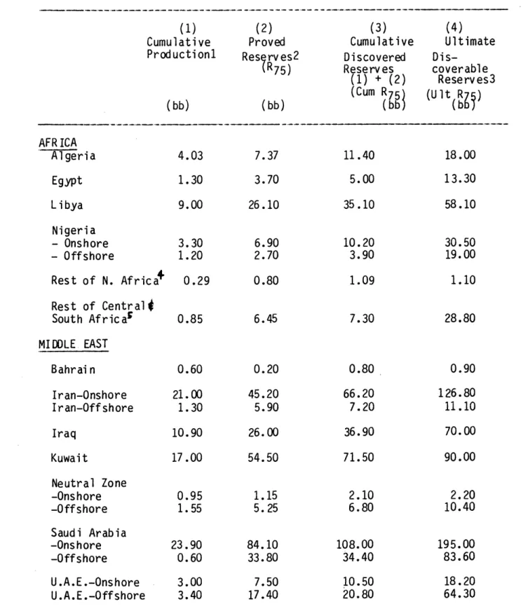
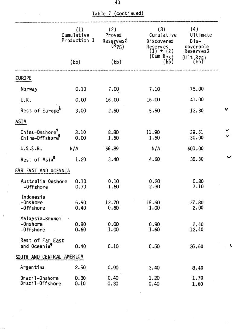
Table 7 presents our data for cumulative production, R75, Cum R75,

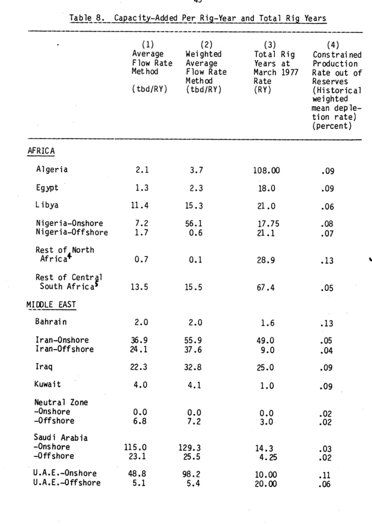
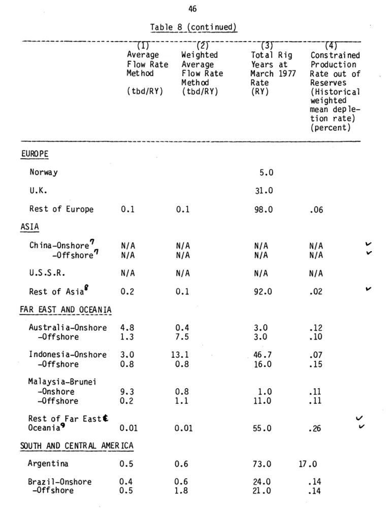
and Ult R75 for use in our model. Table 8 shows the capacity added rates

for both the Average Flow Rate Method (column (1)) and the Weighted Average Flow Rate Method (column (2)). For our model simulation we use the rig-year rates prevailing as of March 1977 (column (3) in Table 8).

Column (4) in Table 8 shows the constrained a used in the model if a* > a. The footnotes to Tables 7 and 8 are an integral part of the data and are contained in Appendix I.

No detailed comments are attempted. Several anomalies are apparent, and serve to make us re-examine data or assumptions, e.g., the 3 percent constraint for Saudi Arabia production, or the decline in drilling there; or the original 1978 capacity, which relates to what the well can

produce, not what the surface facilities can put through.

t

42

Table 7. Production and Reserve Data (as of 12-31-75)

(1) Cumulative Productionl (bb) (2) Proved Reserves2 (R75) (bb) (3) Cumulative Discovered Reserv es (1) + (2) (Cum R7 (bb (4) Ultimate Dis-coverable Reserv es3 (U lt R) (bbJ AFRICA Algeria Egypt Libya Nigeria - Onshore - Offshore Rest of N. Africa+ Rest of Centralt South Africa! MIDDLE EAST Bahrai n Iran-Onshore Iran-Off shore Iraq Kuwait Neutral Zone -Onshore -Offshore Saudi Arabia -Onshore -Offshore U .A.E .- Onshore U.A.E.-Offshore 18.00 13.30 58.10 30.50 19.00 1.10 v 28.80 0.90 126.80 11.10 70.00 90.00 2.20 10.40 195.00 83.60 18.20 64.30 4.03 1.30 9.00 3.30 1.20 0.29 0.85 0.60 21. 00 1.30 10.90 17.00 0.95 1.55 23.90 0.60 3.00 3.40 7.37 3.70 26.10 6.90 2.70 0.80 6.45 0.20 45.20 5.90 26. 00 54.50 1.15 5.25 84.10 33.80 7.50 17.40 11.40 5.00 35.10 10.20 3.90 1.09 7.30 0.80 66.20 7.20 36.90 71.50 2.10 6.80 108.00 34.40 10.50 20.80 '-"I- --- -·111111---)1-·--- T

Table 7 (conti nued) (1) Cumulative Production (bb) (2) Proved Reserves2 (R75) 1 (bb) (3) Cumulative Discovered Rese rv es (1) + (2) (Cum R7 (b91 (4) Ultimate Dis-coverable Reserves3 (Ult R) (bbl Norway U.K. Rest of Europe' ASIA Ch ina-Onshore' Chi na-Off shorer U.S.S.R. Rest of Asia8 0.10 0.00 3.00 3.10 0.00 N/A 1.20 FAR EAST AND OCEANIA

Australia-Onshore 0.1 -Offshore 0.71 Indonesia -Onshore 5.91 -Offshore 0.41 Malaysia-Brunei -Onshore O.9( -Offshore 0.6(

Rest of Far East

and Oceania9 0.4(

SOUTH AND CENTRAL AMERICA

Argentina 2.5( Brazil-Onshore 0.8( Brazil-Offshore 0.1( 0 ) ) ) ) 0 ) ) ) EUROPE 75.00 41.00 13.30 7.00 16.00 2.50 8.80 1.50 66.89 3.40 0.10 1.60 V 39.51 30.00 V V 7.10 16.00 5.50 11.90 1.50 N/A 4.60 0.20 2.30 18.60 1.00 0.90 1.60 0.50 3.40 1.20 0.40 600.00 38.30 0.80 7.10 37.80 2.00 2.40 12.40 12.70 0.60 0.00 1.00 0.10 36.60 V 0.90 0.40 0.30 8.40 1.70 1.60 - --- - ---

-44 Cumulative Production 1 (bb) Table 7 (continued) Proved Reserves2 (R7 5) (bb) (3) Cumulative Discovered Rese rv es (1) + (2) (Cum R75 (bb (4) Ultimate Dis-coverable Rese rv es3 (Ult(R7) (bb

SOUTH AND CENTRAL AMERICA (continued)

Mexico-Reforma ° 0.10 6.00

Mex ico-Otherle 4.70 1.30

Venezuela

-Ons hore 17.40 10.90

-Offshore 14.70 4.60

Rest of South and

Central America" 5.10 4.90 NORTH AMERICA Canada Crude Oil NGL* Tot al USA (lower 48) Crude Oil NGL* Total Alaska Total USA 7.44 0.90 8.30 108.33 15.69 124.02 0.68 124.70 6.65 1.59 8.24 32.70 6.27 38.97 10.00 48.97 *Natural gas footnote 12).

liquids-data are as of 12/31/74 from API and CPA (see Numbered footnotes are in Appendix I.

90.00 6.50 V VY 6.10 6.00 28.30 19.30 10.00 54.60 20.00 25.80 V 14.09 2.49 16 .54 141 .03 21.96 162.99 10.68 17 3.67 65.80 2.73 68.53 218.13 218.13 10.72 228.85

Table 8. Capacity-Added Per Rig-Year and Total Rig Years

(1) (2) (3) (4)

Average Weighted Total Rig Constrained

Flow Rate Average Years at Production

Method Flow Rate March 1977 Rate out of

Method Rate Reserves

(tbd/RY) (tbd/RY) (RY) (Historical

weighted mean deple-tion rate) (percent) AFRICA Algeria Egypt L i bya Nigeria-Onshore Nigeria-Offshore Rest of North Afric as Rest of Central South Africa' MIDDLE EAST Bahrain Iran-Onshore Iran-Off shore Iraq Kuwait Neutral Zone -Onshore -Offshore Saudi Arabia -Onshore -Offshore U.A.E.-Onshore U.A.E.-Offshore 2.1 1.3 11.4 7.2 1.7 0.7 13.5 3.7 2.3 15.3 56.1 0.6 0.1 15.5 2.0 36.9 24.1 22.3 4.0 0.0 6.8 115.0 23.1 48.8 5.1 2.0 55.9 37.6 32.8 4.1 0.0 7.2 129.3 25.5 98.2 5.4 108.00 18.0 21 .0 17.75 21.1 28.9 67.4 1.6 49.0 9.0 25.0 1.0 0.0 3.0 14.3 4.25 10.00 20.00 .09 .09 .06 .08 .07 .13 .05 .13 .05 .04 .09 .09 .02 .02 .03 .02 .11 .06 V