EXPERIMENTAL INVESTIGATION OF SELF-EXCITED
INDUCTION GENERATOR FOR INSULATED WIND TURBINE
Nadir Kabache Samir Moulahoum Hamza Houassine Research Laboratory on Electrical Engineering and Automatics, LREA
University of Médéa, 26000, ALGERIA
Tel: +21325599986 Fax : +21325599986 Emails: nadir.kabache@gmail.com kabache.nadir@univ-medea.dz samir.moulahoum@gmail.com moulahoum.samir@univ-medea.dz hamza_houassine@yahoo.fr houassine.hamza@univ-medea.dz
Abstract – The use of induction machine in autonomous operating mode of wind turbine generators is very appreciated in many applications for economic, logistic and technical issues. However, the induction machine model, which is naturally nonlinear, becomes more complicated with the addition of external capacitive bank for the self-excitation of the machine. The present paper provides a theoretical and experimental investigation of a self-excited induction generator (SEIG) behavior for various connection topologies by considering the machine magnetic saturation. A good agreement between simulation and experimental result is obtained from the benchmark test which includes various balanced and unbalanced loads with and without power convert.
Keywords: Induction generator, self-excitation, magnetic saturation, power inverter, variable load.
1. Introduction
Compared to other electrical machine, the induction machine is rugged, reliable, low cost and maintenance free. For that it is widely used in almost of industrial applications, in particular, to equip wind turbine generator for small powers plants. Two configurations can be expected for the use of the induction machine in wind turbine generator, connected to the main grid or stand-alone operation. While the magnetizing reactive power needed to excite the generator is provided by the grid in the connected case, in the stand-alone operating mode, there is no external reactive power and the generator must be self-excited. Practically this problem can be solved by connecting appropriate capacitors bank with the machine winding. Such operating mode is much appreciated because it allows autonomous generator and therefore, decentralized electrical sources [1]. However, the SEIG dynamical behavior become more complicated since voltage and frequency can be affected considerably by the wind speed, the exciting capacitance and the variation in load demand [2].
Furthermore, while the saturation is neglected in motor
operating mode to achieve best performances, it must be considerate in the SEIG model. Indeed, during the self-excitation, the variation in magnetizing inductance due to saturation is the main factor that stabilizes the growing transient of generated voltage [3-4].
This paper gives a simulation and experimental analysis for the behavior of a self-excited induction generator under some kinds of balanced and unbalanced load. Firstly, the model of the induction generator with magnetic saturation is established including the model of the self-excitation capacities as well as that of the load (linear and nonlinear load). The saturation effect is associated with the magnetizing flux by expressing the leakage flux and their time derivatives, in synchronous frame, as a function of currents. Thereafter; the resulting model is simulated for different operating mode with and without power inverter. Final and to check the validity of the suggested approach, an experimental test is done. The obtained result show a good agreement between simulation and experimental tests for all considered operating mode.
2. Self Excited Induction Generator Modeling 2.1 Induction machine model
The transient behavior of an induction machine is normally represented in the d-q reference. As illustrated in Fig. 1, a resistor RFe coupled to the magnetizing branch is added to incorporate iron losses. This resistor can be used to takes into account core losses in stator iron. Core losses in rotor are not correct represented by RFe and are neglected in this paper [5].
The dynamic model of the induction machine in the synchronous reference frame is described by the following equations: Vs R Is s d s/dt js (1) s Vr R Ir r d r/dt jsl (2) r R IFe Fe d m/dtjsm (3) s L Is s m , m L Im m (4) r L Ir r m , ImIFe (5) Is Ir ( ) ( ) / em m dr qs qFe qr ds dFe r T PL I I I I L (6) The symbols in (1)-(6) are defined as:
,
s r
R R Stator and rotor resistances;
,
s r
L L Stator and rotor leakage inductances;
m
L Mutual inductance;
,
s r
Stator and rotor flux vectors; ,
s r
V V Stator and rotor voltage vectors;
,
s r
I I Stator and rotor currents vectors;
,
m Im
Magnetizing flux and current vectors; ,
s sl
Synchronous and slip angular speeds; P Number of pole’s pair;
em
T Electromagnetic torque;
Fe Index associated to iron loss branch. Consideration of iron loss leads to an increase of the system order and introduces additional mutual coupling between the axis components d and q.
The use of saturation has been investigated in several works and some methods are suggested [3-7]. In this paper, Saturation effect in induction machines is associated with the magnetizing flux, whereas, saturation of leakage flux is neglected. Including saturation in d-q axis model consists of expressing the flux linkages and their time derivatives as function of currents
The principles of magnetizing flux saturation modeling and derivation procedure remain the same as for induction machine without iron loss. The function Lm=F(Im), which models saturation, is applied to the set of equations (1-6). Model of a saturated induction machine can be formed in
various different ways, depending on the selected set of state-space variables [4]. The model selected here is the one with stator and rotor current d–q axis components as state-space variables. It may be given in matrix form as [5]:
V L I R I (7) s I r I Fe I Im RFe Lm Lr Ls Rr Rs s s s j L I + s m m j L I s r r j L I r r j s VFig. 1. Equivalent circuit of an induction machine by
considering saturation and iron losses (7) s s s s m s m s s s s m s m sl m r sl r sl m sl m sl r r sl m s m s m Fe s m s m s m s m Fe R L 0 L 0 L L R L 0 L 0 0 L R L 0 L R L 0 L R L 0 0 L 0 L R L L 0 L 0 L R
The variable terms in (7) are: 2 2 cos sin d dy m M M L 2 2 sin cos q dy m M M L (8) Mdq(MdyLm) cos sin
Mdy and Lm are the dynamic and the static mutual inductance's, respectively. Mdq is the term that explains the "cross effect" between the axis in quadrate. α is the angle between the d axis and the magnetizing current Im.
From a practical point of view the developed model can be easily used. It requires only a preliminary experimental evaluation of the no-load magnetizing characteristic of the machine Lm=F(Im) (Fig.2. and Fig.3.) and the equivalent iron loss resistance RFe. The evaluation can be made by performing standard no-load tests on an
V Vds,Vqs, 0, 0, 0, 0T
I Ids,Iqs,Idr,Iqr,IdFe,IqFeT s d dq d dq d dq dq s q dq q dq q d dq r d dq d dq dq q dq r q dq q d dq d dq d dq dq q dq q dq q L M M M M M M M L M M M M M M M L M M M M L M M M L M M M M M M M M M M M M M M M Fig. 2. Magnetizing inductance versus magnetizing current
Fig. 3. Magnetizing inductance versus phase voltage
induction machine. Therefore in the following analysis the parameters of the induction machine are assumed constant except the magnetizing inductance which varies with saturation.
In generator operating conditions, equations (1-6) cannot be solved because the voltage space Vs is not known; it is possible to obtain solution only with an external network that provides reactive power. In the self excited induction generator, this power is obtained form a capacitance bank.
2.2 Self-exciting capacities model
The model of capacities of self-excitation is established in a way completely independent of the machine model. The stator windings of the induction generator are connected to a star capacitive bank. The equations of self excitation, at no load conditions, are given by:
1 1 , , js jsg jc dV I I j a b c dt c c (9)
Where Isg is the generator current (magnetizing current), Ic is the capacitance current, and a, b, c are phases indices. In the no-load conditions, the generator current is
equal to the capacitance current (Fig. 4).
This system can be transformed in the synchronous reference frame (d,q) by applying Park Transformation:
1 1 ds dsg s qs qs qsg s ds dV I V dt c dV I V dt c (10)
The value of the excitation capacitance must be greater than a minimum limit so that the generator current is sufficient for the operation in the nonlinear portion of the magnetization curve.
2.3 Model of the used Load with the SEIG
To check the performances of the SEIG some linear and nonlinear load were used (Fig. 4). For the linear case the SEIG is loaded by bank of resistance, inductance and capacity. For the nonlinear case, an association of three phase diode bridge rectifier and DC-AC converter is used.
In the case of linear load, the dynamic model of a three-phase balanced load can be expressed as:
1 , , jsL js L jsL L jsL L dI V R I L I dt j a b c dt C
(11)Where IsL is the load current, and RL, LL, CL are the load components. Hence, the self excitation model takes the followings form at load conditions (Fig. 4):
1 ( ) 1 ( ) ds dsg dsL s qs qs qsg qsL s ds dV I I V dt c dV I I V dt c (12) In the case of nonlinear load, with a diode bridge rectifier, the output voltage is expressed as:
0 0.2 0.4 0.6 0.8 1 1.2 1.4 0 0.2 0.4 0.6 0.8 1 1.2 Magnetizing current(A) Magnetizing Inductance(H) Experimental points Interpolation 0 50 100 150 200 250 300 0 0.2 0.4 0.6 0.8 1 1.2 Voltage(V) Magnetizing Inductance(H) Experimental points Interpolation
Fig. 4. The Selected load for the self-excited induction generator
Rectifier DC-AC Converter RLC Load Capacitance Bank SEIG D1 D1' D2 D2' D3 D3' T1 T1' T2 T2' T3 T3' Id Cf C Generator
current Load current
Capacitance current
( ) ( ), , ,
d js js
U Max v Min v j a b c (13) The Dc Link current is governed by the following equation: d d L L U I L s R (14) Where, RL and LL are the load resistance and inductance respectively.
Then, the Load current that fed the rectifier is deduced:
' ' 1,2,3 2,3,1 3,1,2 ' , , 1,2,3 2,3,1 3,1,2 if and ( ou ) are On if et ( ou ) are On 0 if not d asL bsL csL d I D D D I I D D D (15)
The equations (12) remain still valid.
Finally, the SEIG feed an association including an electronic converter, an inverter and RL load. The PWM signals are used to switch on the IGBT’s in the converter. This converter is modeled by three switching functions (F1, F2 and F3) to determinate the state of the IGBTs (on or off) in each arm of the bridge. Considering the commutation basic rules of converters, the switches of a arm must change of complementary form. Fi is the switching functions to determinate the state of IGBTs:
' ' 1 i f i s O n a n d i s O f f 0 i f i s O n a n d i s O f f i i i i i T T F T T (16)
The converter output voltages, applied to the load, are given by: 1 2 3 2 1 3 3 2 1 (2 ) / 3 (2 ) / 3 (2 ) / 3 asL f bsL f csL f V U F F F V U F F F V U F F F (17)
The differential voltage equations of the inverter are as follow: asL asL L L asL bsL bsL L L bsL csL csL L L csL dI V L R I dt dI V L R I dt dI V L R I dt (18)
The dc side current of the inverter and its relationships with the ac side currents is expressed by:
Id F i1 a s L 2F ib s L 3F i (19) c s L
3. Simulation and experimental results
Many examples of simulation test cases have been studied to evaluate the modeling approach. A select few are presented in this section. The experimental bench has been realized with an induction generator mechanically coupled with a dc motor. Linear loads, capacitance bank, numerical scope with PC connection complete the bench (Fig. 5). The experiments investigated in this section are done in no-load and loading conditions with linear loads. The data acquisition started a short time before the built up process or load application.
A 0.37 kW induction machine is used for simulation and experimental investigations (data are given in appendix). The induction generator is operated at 1500 rpm driven by a DC motor as a prime mover. Then a star connected capacitor bank of 8,4μF was switched across the terminals of the stator of the induction machine. The excitation capacitors are selected to provide the generator rated terminal voltage at no load condition.
Induction generator
Current and voltage Measurments PC
Scope
DC Motor mover Converter
Fig. 5. Experimental bench
3.1 No-load operation
The operation of the asynchronous generator, based on a simplified model (not taken into account of saturation), leads to a divergence of the characteristics because the saturation which fixes the operating point in steady operation.
Self-excitation is excited by reciprocal relation of rotor residual magnetism and self-excited capacitor. When the machine is driven by an external mover, the current is induced in the stator winding because of residual flux of the rotor. Connection of suitable capacitors to stator winding causes leading current. This current increases the core flux, and the voltage difference between induction voltage and capacitors can be constant. The continuous increasing of voltage is controlled by magnetic saturation and voltage finally reaches steady state. The voltage depends on speed, capacitance, machine parameters, magnetic characteristics and loads. Such magnetic excitation phenomena are caused by continuous energy circulation between the electric field (capacitors) and the magnetic field (machine). When the operating point is reached, the machine delivers a stator voltage which its rms value is constant.
Fig. 6 shows the experimental voltage and current recorded by numerical scope, signal acquisition is done by differential sensors with 400V/2.5V scale for the voltage and 0.5V/2A for the current. However, in order to verify the proposed model and compared the simulated and experimental curves, the data acquisition is converted to its real value and used to plot the experimental curves with the same scale as the simulated ones.
Fig. 7 shows the simulated and experimental build-up of voltage achieved when 8.4μF of capacitance was switched across the motor stator winding while it was turning at 1500 rpm. Fig. 8 shows the simulated and experimental built up process of the stator current under no-load conditions. As can be observed, the magnitude of the voltage and the current obtained experimentally are in agreement with the simulated ones. As can be observed in Fig. 9, the magnetizing inductance starts from a smaller value then increases to reach its peak value and finally starts to drop. This change in Lm is due to the characteristics of the magnetizing curve seen in Fig. 3, at the start of self- excitation point where the voltage is close to zero, Lm is close to its linear value. Once self-excitation starts the generated voltage will grow and then Lm also increases up and then Lm starts to decrease while the voltage continues to grow until it reaches its steady state value.
Fig. 10 shows the variation of the rms generator voltage against the variations in the speed and excitation capacitors. As can be seen, the rms generator voltage increases as the values of the self-excitation capacitor and speed increase. Increasing self excitation capacitance value results in high voltage. Therefore, the capacitance value must be correctly adjusted.
Fig. 6. Generator voltage and current built up process at no-load recorded experimentally
Fig. 7. Generator voltage built up process at no-load - Simulation (high) - Experimental (low)
Fig. 8. Generator current built up process at no-load - Simulation (high) - Experimental (low)
0 0.5 1 1.5 2 2.5 -300 -200 -100 0 100 200 300 time(s) Voltage (V) 0 0.5 1 1.5 2 -300 -200 -100 0 100 200 300 time(s) Voltage (V) 0 0.5 1 1.5 2 2.5 -1 -0.8 -0.6 -0.4 -0.2 0 0.2 0.4 0.6 0.8 1 time(s) Current (A) 0 0.5 1 1.5 2 -1 -0.8 -0.6 -0.4 -0.2 0 0.2 0.4 0.6 0.8 1 time(s) current (A)
Fig. 9. Magnetizing inductance during built up process at no-load
Fig. 10. Evolution of the rms generator voltage depending on the
speed and excitation capacities (Experimental points with interpolation)
Fig. 11. Sudden disconnection of one of the three excitation
capacitors: voltage maintenance
Fig. 12. Sudden disconnection of one of the three excitation
capacitors: voltage fall down
Fig. 13. Unbalanced capacities effect - Simulation (high) - Experimental (low)
When one of the three capacities is sudden disconnected, the process of self-excitation is maintained if the value of two remaining capacities is sufficient to maintain the stator voltage (Fig. 11). If the unbalanced operation, obtained with the two remaining capacities, is not sufficient to maintain the phenomenon of self-excitation, the accumulated reactive energy slowly disappears and consequently the voltage amplitude slowly decreases to a very low level, hence, the stator voltage falls down and causes the demagnetization of the generator (Fig. 12). Furthermore, unbalanced excitation capacities lead to an unbalanced stator voltage as shown in Fig. 13.
0 0.5 1 1.5 2 2.5 0.5 0.6 0.7 0.8 0.9 1 1.1 1.2 1.3 time(s) Magnetizing inductance(H) 4 5 6 7 8 9 10 0 50 100 150 200 250 300 350
Capacity (Micro Farad) Voltage (Volt) 1500 rpm 1600 rpm 1700 rpm 1800 rpm 12000 1300 1400 1500 1600 1700 1800 1900 2000 50 100 150 200 250 300 350 400 Speed (rpm) Voltage (Volt) C = 6.08 Micro Farad C = 7.06 Micro Farad C = 8.26 Micro Farad C = 9.08 Micro Farad C = 9.76 Micro Farad 0 0.5 1 1.5 2 2.5 -300 -200 -100 0 100 200 300 time(s) Voltage (V) 0 0.5 1 1.5 2 2.5 -300 -200 -100 0 100 200 300 time(s) Voltage (V) 0.68 0.7 0.72 0.74 0.76 0.78 -400 -300 -200 -100 0 100 200 300 400 time(s) Voltage (V) 0.7 0.72 0.74 0.76 0.78 -300 -200 -100 0 100 200 300 time(s) Voltage (V)
3.2 Load operation
Two possible connections of the induction generator to load can be found: either connected on the load directly or by means of an electronic converter. The first one has advantages of costs, maintenance and reliability while the second one, by making speed regulation possible, increases the efficiency of the wind turbines [8,9].
3.2.1 Linear load
The call of reactive energy, poses a problem for the induction generator. Because, even for its own requirements in reactive, it depends on an external source (capacities of excitation). The more important the load is, the more the requirement in reactive energy of the induction generator is important, which results in a decrease of the output generator voltage (Fig. 14 to Fig 17). Without load the SEIG requires only its own reactive power for self-excitation, but loaded SEIG requires a more reactive power for self-excitation and for inductive load. When Rand L is large the characteristic is similar to the no load self excitation case. If R-L is small, larger is the load.
In load tests, immediately after that a transient process started, the voltage and current amplitude rapidly decreased. The generator decelerates; the reason for the decrease in rotational speed is due to the change in load torque, as a result a slightly frequency decrease after the load application is detected.
Fig. 14. Generator voltage response to resistive load
connection at t=0.45s - Simulation (high) - Experimental (low)
Fig. 15. Generator current response to resistive load
connection at t=0.45s - Simulation (high) - Experimental (low)
Fig. 16. Load current response
- Simulation (high) - Experimental (low)
0 0.5 1 1.5 2 2.5 -300 -200 -100 0 100 200 300 time(s) Voltage (V) 0 0.5 1 1.5 2 -300 -200 -100 0 100 200 300 time(s) Voltage (V) 0 0.5 1 1.5 2 2.5 -1 -0.8 -0.6 -0.4 -0.2 0 0.2 0.4 0.6 0.8 1 time(s) Current (A) 0 0.5 1 1.5 2 -1 -0.8 -0.6 -0.4 -0.2 0 0.2 0.4 0.6 0.8 1 time(s) Current (A) 0 0.5 1 1.5 2 2.5 -0.25 -0.2 -0.15 -0.1 -0.05 0 0.05 0.1 0.15 0.2 0.25 time(s) Load Current(A) 0 0.5 1 1.5 2 -0.25 -0.2 -0.15 -0.1 -0.05 0 0.05 0.1 0.15 0.2 0.25 time(s) Current (A)
Fig. 17. Simulation of Generator voltage and current response
to inductive load connection at t=0.45s
As can be seen form Fig. 18, the generator voltage decreases when the value of the load impedance Z decreases, in other hand, it indicates that the generator voltage tends to fall steeply with balanced inductive load as compared with the resistive load (when cos decrease, generator voltage is more affected). With inductive load, excitation capacitors must provide the reactive power to the inductive load in addition to the reactive power to the generator.
To compensate the supplement of reactive called by the generator, one can insert series condensers with the load (Fig. 19 and 20). This technique of compensation is a simple method to improve the generator voltage regulation.
Fig. 21 shows the behavior of SEIG under an unbalanced load. In this case, the generated voltage and its frequency decrease. Moreover, the three phase terminal voltage and stator currents are also unbalanced [10-11]. As a result of this unbalanced currents yield a current that flow by the neutral conductor if existed.
Fig. 18. Evolution of the generator voltage depending on the
value of the impedance Z (left) and the power factor cos (right)
Fig. 19. Generator voltage response to capacitive load connection
- Simulation (high) - Experimental (low)
Fig. 20. Generator current response to capacitive load connection
- Simulation (high) - Experimental (low)
0 0.5 1 1.5 2 2.5 -300 -200 -100 0 100 200 300 time(s) Voltage(V) 0 0.5 1 1.5 2 2.5 -1 -0.8 -0.6 -0.4 -0.2 0 0.2 0.4 0.6 0.8 1 time(s) Current(A) 1 1.5 2 2.5 120 140 160 180 200 220 240 time(s) Rms Voltage(V) Z= 530 Ohms Z= 2630 Ohms Z= 790 Ohms 1 1.5 2 2.5 170 180 190 200 210 220 230 240 250 time(s) Rms Voltage(V) Power factor= 0.85 Power factor= 0.75 Power factor= 0.65 0 0.5 1 1.5 2 2.5 -300 -200 -100 0 100 200 300 time(s) Voltage(V) 0 0.5 1 1.5 2 -300 -200 -100 0 100 200 300 time(s) Voltage (V) 0 0.5 1 1.5 2 2.5 -1 -0.8 -0.6 -0.4 -0.2 0 0.2 0.4 0.6 0.8 1 time(s) Current(A) 0 0.5 1 1.5 2 -1 -0.8 -0.6 -0.4 -0.2 0 0.2 0.4 0.6 0.8 1 time(s) Current (A)
Fig. 21. Voltage for unbalanced load - Simulation (high) - Experimental (low) 3.2.2 Non linear load
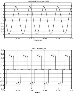
In Figures 22, 23 and 24, the generator and load currents in case of diode rectifier, thyristor rectifier or converter insertion, are respectively presented.
Fig. 22. Generator and Load currents in case of a diode
Fig. 23. Generator and Load currents in case of a thyristor
rectifier+RL load with =30°
Fig. 24. Generator and Load currents in case of a
rectifier+converter+RL load 1.06 1.08 1.1 1.12 1.14 1.16 -300 -200 -100 0 100 200 300 time(s) Voltage(V) 1.08 1.1 1.12 1.14 1.16 -300 -200 -100 0 100 200 300 time(s) Voltage (V) 2 2.02 2.04 2.06 2.08 2.1 -1 -0.8 -0.6 -0.4 -0.2 0 0.2 0.4 0.6 0.8 1 time(s) Generator current(A) 2 2.02 2.04 2.06 2.08 2.1 -0.5 -0.4 -0.3 -0.2 -0.1 0 0.1 0.2 0.3 0.4 0.5 time(s) Load Current(A) 2 2.02 2.04 2.06 2.08 2.1 -0.8 -0.6 -0.4 -0.2 0 0.2 0.4 0.6 0.8 time(s) Generator current(A) 1.9 1.92 1.94 1.96 1.98 2 -0.5 -0.4 -0.3 -0.2 -0.1 0 0.1 0.2 0.3 0.4 0.5 time(s) Load Current(A) 1.9 1.92 1.94 1.96 1.98 2 -1 -0.8 -0.6 -0.4 -0.2 0 0.2 0.4 0.6 0.8 1 time(s) Generator current(A) 1.9 1.92 1.94 1.96 1.98 2 -0.25 -0.2 -0.15 -0.1 -0.05 0 0.05 0.1 0.15 0.2 0.25 time(s) Load Current(A)
After non linear load application, figures show that generator and load currents present a high low-order harmonic content, due to the presence of the converter. Before and after load application, the harmonic content in the currents has been slightly changed. It can be seen from these figures that for both the rectifier and the converter, the generator current wave form is distorted and becomes not sinusoidal [12-13]. The THD is about 6.43 %, 6.42 % and 14.85 % for the three nonlinear loads respectively. However, in the case of inverter, the generator output voltage of the generator is rectified and inverted using the PWM inverter. The modulation index is adjusted such that the voltage and the frequency at the output are maintained. 5. Conclusion
In this paper, modeling of the self-excited induction generator used in wind generation was investigated. The developed model has been validated by experimental results. The analysis of the results presented in the paper clearly evidences that saturation phenomena have a considerable effect on the performances and must be taken into account. The limits relate to the variations of the rms voltage and the frequency at load application and the possible variations of speed were outlined. The behavior of the induction generator depends considerably on the load, in the case of a linear load, the output voltage as well as the current decrease but remain sinusoidal. Whereas, in the case of nonlinear load, a bad quality of the energy is related to the no-sinusoidal form of the voltage wave because of the presence of a static converter. However, the voltage level and the frequency at the output can be maintained.
Appendix: The parameters of the induction machine
Rated machine power 0.37 KW
Rated speed 1380 rpm
Rated voltage 400/230 V
Stator resistance Rs 23 Ω
Rotor resistance Rr 21,21 Ω Iron loss equivalent resisrance RFe 2936Ω Stator Leakage inductance Ls 0,0684 H Rotor Leakage inductance Lr 0,0684 H
Inertia J 0,0024 kg.m2
Friction coefficient F 0,000012kg.m²/s
References
[1] S.S. Murthy, B.P. Singh, C. Nagamani and K.V.V. Atyanarayana, “Studies on the use of conventional Induction motors as self-excited induction generators” IEEE trans. on energy
conversion, Vol. 3, No. 4, 1988, pp.842-848.
[2] G.K. Singh, "Self-excited induction generator research – A survey," Electric Power Systems
Research, Vol. 69, 2004, pp. 107-114.
[3] L. Boldea, S.A. Nasar, "Unified treatment of core losses and saturation in the orthogonal-axis model of electric machines," IEE Proceedings, Pt. B, Vol. 134, No. 6, 1987, pp. 355-363.
[4] E. Levi, "A unified approach to main flux saturation modelling in D-Q axis models of induction machines," IEEE Transactions on Energy Conversion, Vol. 10, No. 3, 1995, pp. 455-461.
[5] S. Moulahoum, O. Touhami, "Sensorless Vector Controlled Induction Machine in Field Weakening Region: Comparing MRAS and ANN-Based Speed Estimators ", Journal of Electrical Engineering &
Technology, JEET, Korean Institute of Electrical Engineering, KIEE, Vol: 2, N°: 2, 2007, pp 241-248.
[6] S. Moulahoum, L. Baghli, A. Rezzoug, O Touhami, "Sensorless Vector Control of a Saturated Induction Machine accounting for iron loss", European journal
of Electrical engineering, EJEE, Lavoisier, Hermès
Sciences, Vol : 11, N° :4/5, 2008, pp 511-543. [7] A. Garg, K. S. Sandhu: Dynamic Simulation, Analysis
and Control of Self-excited Induction Generator Using State Space Approach. Journal of Electrical Engineering JEE, Vol.13, No.2, June 2013.
[8] D. Iannuzzi, E. Pagano,L. Piegari, O. Veneri "Generator operations of asynchronous induction machines connected to ac or dc active/passive electrical networks," Mathematics and Computers in
Simulation, Elsevier, Vol. 63, 2003, pp 449–459.
[9] Dawit S Eyaum Colin Grantham, and Muhammed Fazlur Rahman,”The dynamic characteristics of an isolated self-excited induction generator driven by a wind turbine”, IEEE, Transaction on Industry
applications, Vol. 39.No.4, 2003, pp 936 - 944.
[10] Radosavljević Jordan, Klimenta, Dardan, Jevtić, Miroljub.: Steady-State Analysis of Parallel-Operated Self-Excited Induction Generators Supplying an Unbalanced Load. Journal of Electrical Engineering, Vol. 12, No.4, pp.213–223, September 2012.
[11] Po-Hsu Huang; El Moursi, M..S. ; Weidong Xiao ; Kirtley, J.L., “Fault Ride-Through Configuration and Transient Management Scheme for Self-Excited Induction Generator-Based Wind Turbine”, IEEE Transactions on Sustainable Energy, Volume:5 , N: 1, Jan, 2014, P: 148-159.
[12] Wang, L. ; Lee, D.-J., “Coordination Control of an AC-to-DC Converter and a Switched Excitation Capacitor Bank for an Autonomous Self-Excited Induction Generators in Renewable-Energy Systems”, IEEE Transactions on Industry Applications, Volume N: 99, Jan. 2014.
[13] SarsingGao;Bhuvaneswari, G. ; Murthy, S.S. ; Kalla, U., “Efficient voltage regulation scheme for three-phase self-excited induction generator feeding single-phase load in remote locations”, IET, Renewable Power Generation, Volume:8 , N: 2 , March 2014, P:100 – 108.