Adjoint-based optimization of U-bend channel flow using a multi-fidelity eddy viscosity turbulence model

Adjoint-Based Optimization of U-Bend Channel

Flow Using a Multi-Fidelity Eddy Viscosity

Turbulence

Model

MASSACHUSETTS INSTITUTE

OF TECHNOLOGY

by

JUL

1i 1Z2l1

Michael

Elia Hayek

L

11201E

LIBRARIES

B.S., University of Massachusetts Amherst (2009)

ARCHIVES

Submitted to the Department of Aeronautics and Astronautics

in partial fulfillment of the requirements for the degree of

Master of Science

at the

MASSACHUSETTS INSTITUTE OF TECHNOLOGY

June 2017

Massachusetts Institute of Technology 2017. All rights reserved.

Auho...Signature

red acted

A uth or ... ...

Department of Aeronautics and Astronautics

May 25, 2017

Certified by ...

Signature

redacted

Qiqi

Wang

Associate Professor of Aeronautics and Astronautics

Thesis Supervisor

Accepted by ...

redacted

Youssef M. Marzouk

Associate Professor of Aeronautics and Astronautics

Chair, Graduate Program Committee

Adjoint-Based Optimization of U-Bend Channel Flow Using a

Multi-Fidelity Eddy Viscosity Turbulence Model

by

Michael Elia Hayek

Submitted to the Department of Aeronautics and Astronautics on May 25, 2017, in partial fulfillment of the

requirements for the degree of Master of Science

Abstract

Many fluid flows in engineering are turbulent and require the use of computational fluid dynamics (CFD) for design purposes. Optimization with CFD has largely been limited to low-fidelity simulation methods, such as Reynolds Averaged Navier Stokes (RANS), due to current computational capabilities. However, RANS has been shown to lack sufficient accuracy for certain flows. This thesis presents CFD simulation of a 180 degree U-bend square duct using low-fidelity steady RANS and high-fidelity wall-resolved Large Eddy Simulation (LES) models. The LES solution is shown to match experimental results, whereas the RANS solution is not sufficiently accurate. A process for training a RANS eddy viscosity field using the LES solution is provided. This approach is based on solving an inference problem by comparing the RANS cal-culations to the LES solution and tuning cell-based turbulent viscosity values. This multi-fidelity framework is intended to highlight that high-fidelity solutions can be used to improve even the simplest RANS turbulence models. The adjoint method is used for efficient gradient-based optimization of the turbulent viscosity on a U-bend channel to minimize the velocity solution error. Other objective functions are explored to check the uniqueness of the optimized turbulent viscosity. Sensitivity of the optimized result to the numerical convection scheme is presented to help provide insight for future optimization of turbulence models. The optimized turbulent vis-cosity is also used on a modified U-bend channel to demonstrate the applicability of the method on new geometries.

Thesis Supervisor: Qiqi Wang

Acknowledgments

First and foremost, I would like to thank my advisor Professor Qiqi Wang. No challenge is too grand for Professor Wang. He has always made himself available and provided invaluable ideas and insight. This work would not have been possible without his guidance.

I would like to thank General Electric Aviation for their support. This research was funded by GE through the Advanced Courses in Engineering, under the supervision of Kenneth Gould and Paul Patoulidis. I would also like to thank GE management for allowing me to pursue this degree while employed at GE Aviation. This specifically includes Tyler Hooper, Marcus Ottaviano, Spiro Harbilas, Dan Barber, and Dan Daigle. They have been patient and accommodating during my extended time at MIT.

I would also like to thank Greg Laskowski, who has been my GE research advisor and has generously offered his time to review my work. Our regular meetings have provided valuable understanding and direction to the research.

Additional appreciation goes to current and former ACDL group members, namely Chaitanya Talnikar and Han Chen for enduring countless questions and sharing their knowledge.

I would like to thank my parents, Jay and Nora, and the rest of my family for their constant support throughout my time at MIT and my academic career. Finally, I would like to thank my wife Jenna, who has always been very loving, patient, and understanding. The completion of this thesis would not have been possible without her continual encouragement.

Contents

1 Introduction ₂₁

1.1 _{Motivation . . . . 21}

1.2 _{Background and Approach . . . . 23}

1.2.1 _{Applicable Scenarios . . . .} 23

1.2.2 Turbine Airfoil Internal Cooling . . . . 23

1.2.3 _{Approach . . . . 25}

1.3 _{Previous Research . . . . 26}

1.4 Thesis Objectives and Contributions . . . . 29

1.5 Thesis Structure. . . . . 30

2 Methods ₃₃ 2.1 Optimization Methods . . . . 33

2.1.1 _{Gradient Based Optimization . . . . 33}

2.1.2 _{L-BFGS method . . . . 34}

2.2 _{The Adjoint Method . . . . 35}

2.2.1 _{Introduction . . . . 35}

2.2.2 _{Formulation . . . . 36}

2.2.3 _{Automatic Differentiation . . . . 38}

2.3 Turbulence Modeling . . . . 39

2.3.1 _{Introduction . . . . 39}

2.3.2 _{Reynolds Averaged Navier Stokes (RANS) . . . . 42}

2.3.3 _{Large Eddy Simulation (LES) . . . . 45}

3 Simulation of a 1800 U-bend Square Duct 51

3.1 Introduction . . . . 51

3.2 Large Eddy Simulation ... 51

3.2.1 Fluid Solver . . . . 51

3.2.2 Spatial and Temporal Discretization . . . . 53

3.2.3 Mean Field: Time-Averaging . . . . 57

3.2.4 Parallel Computing . . . . 59

3.3 RANS Simulation . . . . 60

3.3.1 Fluid Solver . . . . 60

3.3.2 Simulation Details . . . . 60

3.4 Pre-simulation for Unsteady Inlet Boundary Condition for LES . . . . 62

3.4.1 General Approach . . . . 62

3.4.2 Turbulence Model and Key Parameters . . . . 63

3.4.3 Domain and Mesh . . . . 64

3.4.4 Database and Inlet Mapping . . . . 64

3.4.5 Square Duct Result Comparisons to Previous Research . . . . 65

3.5 U-bend CFD Results . . . . 67

3.6 Comparison to Experimental Data . . . . 72

3.6.1 _{Mean Velocity Magnitude . . . .} 72

3.6.2 Turbulent Kinetic Energy . . . . 75

3.7 C onclusion . . . . 76

4 Optimization of the Turbulent Viscosity for a 180* U-bend Channel 77 4.1 Introduction . . . . 77

4.2 Fluid Solvers . . . . 78

4.2.1 High Fidelity Solver . . . . 78

4.2.2 Low Fidelity Solver . . . . 80

4.3 Low-Fidelity Training Setup - HIFIR Model . . . . 82

4.3.1 Objective Functions . . . . 83

4.4 Baseline Optimization of the Turbulent Viscosity . . . . 4.4.1 _{Adjoint Accuracy and Optimization Convergence . . . . .} 4.4.2 _{Velocity and Pressure Fields . . . .} 4.4.3 _{Turbulent Viscosity Field . . . .} 4.4.4 _{Reynolds Stress and Turbulent Kinetic Energy Production} 4.4.5 Reattachment Location 4.5 4.6 4.7 4.8 4.9 4.10

4.4.6 _{Pressure Drop Across U-bend . . . .} Sensitivity to Convection Scheme . . . . Sensitivity to Objective Function Norm . . . . Impact of Bounds on Turbulent Viscosity . . . . Use of Pressure Mismatch for Objective Function . . Impact of Limited Experimental Data on Optimizatioi C onclusion . . . .. . . .

.1

5 Performance of HIFIR model on Adjusted Geometry 5.1 _{Introduction . . . .} 5.2 Geometry Adjustment and Simulation Methods . . . . 5.2.1 _{New U-bend Geometry . . . .} 5.2.2 _{Simulation Methods . . . .} 5.3 _{LES Solution Comparison . . . .}

5.4 HIFIR Solution on Adjusted U-bend Geometry . .

5.4.1 Velocity and Pressure Fields . . . . 5.4.2 _{Velocity Profiles . . . .} 5.4.3 Reattachment Location and Pressure Drop . . . 5.4.4 Turbulent Viscosity Field . . . . 5.5 Conclusions . . . . 6 Summary, Conclusions, and Future Research

6.1 _{Summary and Conclusions . . . .} 6.2 _{Future Research . . . .} . 85 . 85 87 90 92 . . . . 9 4 . . . . 96 . . . . 97 . . . . 103 . . . . 105 . . . . 107 . . . . 112 . . . . 119 121 . . . . 121 . . . . 122 . . . . 122 . . . . 122 . . . . 123 . . . . 125 . . . . 126 . . . . 127 . . . . 130 . . . . 131 . . . 132 133 133 134

A Low-Memory Calculation of Sensitivity Gradient

B Periodic Domain Height Sensitivity Study for LES of U-bend

Chan-nel ₁₄₃

C Benchmarking of Python 2D Incompressible Flow C.1 Laminar Channel ...

C.2 Lid-Driven Cavity ... C.3 Laminar U-bend Channel ... D Convection Schemes for RANS

D.1 Zonal Blending ... D.2 Global Blending ... D.3 Exponential Blending ... D.4 Hyperbolic Tangent Blending

E Turbulent Viscosity Extraction E. 1 Derivation ...

E.2 Implementation in Paraview .

Solver . . . . . . . . . . . . . . . . . . . . Solver from LES . . . . . . . . 149 149 151 155 159 160 163 165 167 171 171 173 137

List of Figures

1-1 _{Example turbine blade shown with internal passages. Original figure}

courtesy of Lindstrom [19] . . . . 24

1-2 Section of turbine airfoil and idealized duct model . . . . 25

3-1 Domain geometry used for square duct U-bend LES . . . . 54

3-2 Views of the U-bend mesh . . . . 55

3-3 Top view of LES mesh sponge region . . . . 55

3-4 Instantaneous y+ from final timestep of LES . . . . 56

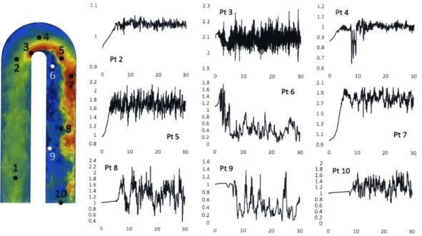
3-5 Instantaneous velocity monitor point data over the first 30 seconds of sim ulation . . . . 57

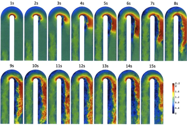
3-6 Instantaneous velocity magnitude at 1 second intervals during start-up, shown at z/dh = 0.5 . . . . 58

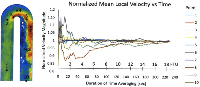
3-7 Normalized local mean velocity as a function of time-averaging duration 59 3-8 Mean velocity field after different durations of time-averaging, shown at z/dh = 0.5. . . . . 59

3-9 Pre-simulation method to create an unsteady inlet boundary condition. 63 3-10 Pre-simulation outlet plane velocity field . . . . 65

3-11 Pre-simulation outlet plane secondary velocity . . . . 66

3-12 Mean velocity magnitude RANS vs LES comparison at z/dh=0.5 . . . 67

3-13 Velocity comparison at two bend sections . . . . 68

3-14 Secondary flow vectors overlaid on mean velocity at two post-bend section s . . . . 70

Turbulent kinetic energy comparison from RANS and LES . . . . Time-averaged velocity magnitude comparison at z/dh=zz0.5 . . . . Bend region mean velocity magnitude comparison at z/dh=0.5 . . Mean velocity magnitude comparison at z/dh=0.03 . . . . PIV vs LES time-averaged velocity magnitude comparison at z/dh: 3-21 Time-averaged TKE* shown at z/dh 0.5

Domain geometry used for U-bend channel LES Mesh used for low-fidelity solver . . . . Convergence of objective value . . . . Comparison of velocity magnitude field . . . . . Comparison of x-velocity field . . . . Comparison of y-velocity field . . . . Comparison of pressure field . . . . Velocity profile at various bend sections . . . . . Comparison of turbulent viscosity ratio field . . 4-1 4-2 4-3 4-4 4-5 4-6 4-7 4-8 4-9 4-10 4-11 4-12 4-13 4-14 4-15 . . . . 78 . . . . 80 . . . . 86 . . . . 87 . . . . 88 . . . . 88 . . . . 89 . . . . 90 . . . . 91 regions . 92 . . . . 93 . . . . 94 . . . . 95 . . . . 96 . . . . 97

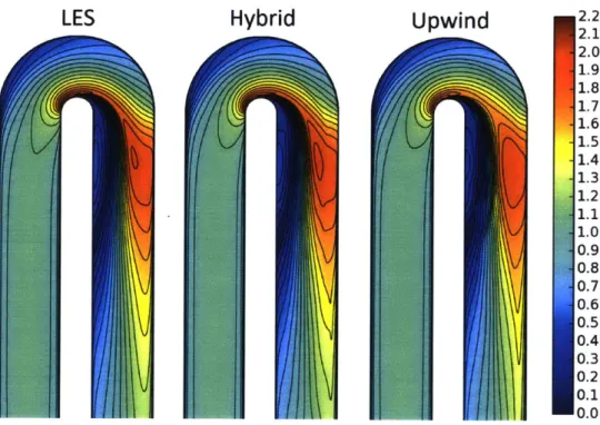
4-16 Comparison of velocity magnitude field for upwind and hybrid schemes 98 4-17 Comparison of pressure field for upwind and hybrid schemes . . . . . 99

4-18 Velocity profile at various bend sections for upwind and hybrid schemes 99 4-19 Velocity profile at bend exit for upwind and hybrid schemes . . . 100

4-20 Comparison of turbulent viscosity ratio field for upwind and hybrid schem es . . . . 101

4-21 Wall shear stress along inner wall in straight exit channel for two con-vection schem es . . . 102 3-16 3-17 3-18 3-19 3-20 71 72 73 74 74 75 0.03

LES turbulent viscosity ratio field and associated negative Comparison of TKE production . . . . Comparison of u'v' Reynolds stress component . . . . Wall shear stress along inner wall in straight exit channel Sections used for pressure drop locations . . . . Convergence of objective value with upwinding . . . .

4-22 Convergence of objective value for Li-based objective function . . . . 104

4-23 Convergence comparison of Li and L2 objective function based on squared L2 solution error . . . 105 4-24 Negative regions of turbulent viscosity shown in blue . . . 106

4-25 Convergence of objective value for pressure mismatch reduction . . . 108

4-26 Comparison of velocity magnitude field for two mismatch reduction m ethods . . . 108 4-27 Comparison of pressure field for two mismatch reduction methods . . 109 4-28 Velocity profile at various bend sections for two mismatch reduction

m ethods . . . 110 4-29 Comparison of turbulent viscosity ratio field for two mismatch

reduc-tion m ethods . . . 110 4-30 Wall shear stress along inner wall in straight exit channel for pressure

reduction m ethod . . . . 4-31 Convergence of objective value for the limited inlet/outlet data case . 113 4-32 Comparison of velocity magnitude field for the limited inlet/outlet data

case ... ... ... 114 4-33 Comparison of pressure field for the limited inlet/outlet data case . . 115 4-34 Velocity profile at various bend sections for the limited inlet/outlet

data case . . . 116 4-35 Velocity profile at a distance of 3H from bend exit . . . 116 4-36 Comparison of turbulent viscosity ratio field for the limited inlet/outlet

data case . . . 117 4-37 Wall shear stress along inner wall in straight exit channel for the limited

inlet/outlet data case . . . 118

5-1 _{Domain geometry used for U-bend channel LES . . . 122} 5-2 _{Comparison of LES velocity magnitude and pressure field for the two}

5-3 Comparison of LES turbulent viscosity ratio and TKE for the two U-bend geom etries . . . . 5-4 Comparison of velocity magnitude field for the adjusted U-bend . . . 5-5 Comparison of pressure field for the adjusted U-bend . . . . 5-6 Velocity profile at various bend sections for the limited inlet/outlet data case. . . . . 5-7 Velocity profile at the bend exit . . . . 5-8 Velocity profile at the domain exit . . . . 5-9 Wall shear stress along inner wall in straight exit channel for adjusted U -b en d . . . . 5-10 Comparison of turbulent viscosity ratio field for the adjusted U-bend

125 126 127 128 129 129 130 131

B-1 Instantaneous velocity showing region of Gortler instability . . . 144

B-2 Domain geometry used for periodic height study . . . 144

B-3 Instantaneous velocity magnitude at three sections . . . 145

B-4 Spanwise velocity magnitude at Section C . . . 146

B-5 Time-averaged velocity comparison between the two periodic height cases ... ... 147

B-6 Time-averaged pressure comparison between the two periodic height cases ... ... 147

C-1 Sketch of straight channel flow . . . . C-2 Python velocity profile vs exact solution for a laminar channel . . . . C-3 Sketch of square lid-driven cavity . . . . C-4 Uniform meshes used for lid-driven cavity grid convergence . . . . C-5 Re 100: velocity profiles along (a) vertical and (b) horizontal lines passing through cavity center . . . . C-6 Re 1000: velocity profiles along (a) vertical and (b) horizontal lines passing through cavity center . . . . C-7 50x50 non-uniform mesh compared to a uniform mesh used for lid driven cavity . . . . 150 151 152 152 153 153 154

C-8 Re = 1000 results for various grid sizes . . . 154 C-9 Re 1000: velocity profiles including non-uniform mesh . . . 155 C-10 Results on a 50 x 50 non-uniform mesh for Re 1 through 1000 . . . . 155 C-11 Laminar U-bend solution: OpenFOAM vs Python . . . 156 C-12 Delta and percent difference plots for laminar U-bend . . . 157 C-13 Streamwise velocity profiles at two bend sections . . . 157 D-1 Example plot of local Peclet number for turbulent U-bend channel . . 161 D-2 Zonal blending: plot of blending factor as a function of Peclet number 162 D-3 Zonal blending: plot of velocity magnitude field for various blending

param eters . . . 162 D-4 Zonal blending: plot of convergence for various blending parameters . 163 D-5 Global blending: plot of velocity magnitude field for various global

blending factor . . . 164 D-6 Global blending: plot of convergence for various global blending factor 164 D-7 Exponential blending: plot of blending factor as a function of Peclet

num ber _{. . . 166} D-8 Exponential blending: plot of velocity magnitude field for various

blend-ing param eters . . . 166 D-9 Exponential blending: plot of convergence for various blending

param-eters ... ... 167 D-10 Hyperbolic tangent blending: plot of blending factor as a function of

Peclet num ber . . . 168 D-11 Hyperbolic tangent blending: plot of velocity magnitude field for

vari-ous blending parameters . . . 169 D-12 Hyperbolic tangent blending: plot of convergence for various blending

List of Tables

3.1 Boundary conditions for LES duct . . . . 53

3.2 Boundary conditions for RANS duct simulation . . . . 61

3.3 Square duct mean flow comparison . . . . 66

4.1 Boundary conditions for LES channel . . . . 79

4.2 Boundary conditions for 2D Python RANS simulation . . . . 81

4.3 _{Comparison of change in objective value . . . . 85}

4.4 Velocity and pressure mismatch from LES . . . . 90

4.5 _{Approximate reattachment location . . . . 96}

4.6 Pressure drop comparison at various inlet and outlet planes . . . . 97

4.7 Approximate reattachment location for pressure reduction method . . 102

4.8 Pressure drop comparison with two HIFIR convection schemes . . . . 102

4.9 Velocity and pressure mismatch from LES for upwind . . . 103

4.10 Approximate reattachment location for pressure reduction method . . 111

4.11 Pressure drop comparison for pressure mismatch reduction . . . 112

4.12 Solution error for the velocity and pressure mismatch reduction methods 112 4.13 Approximate reattachment location for the limited inlet/outlet data case 118 4.14 Pressure drop comparison for limited inlet/outlet data . . . 118

4.15 Solution error for the limited inlet/outlet vs full domain data . . . 119

5.1 Comparison of LES solution for several parameters on the two U-bend geom etries . . . 124

5.2 RANS solution error for the adjusted U-bend geometry . . . 127

5.4 Pressure drop comparison for limited inlet/outlet data . . . 131

A.1 Full vs Low-Memory Adjoint Comparison of 6J . . . 141 B.1 Domain Height Grid . . . 145

Nomenclature

Subscripts b Bulk c Centerline eff Effective 00 Far-field t Turbulent th Threshold w Wall Symbols dh Hydraulic diameter

H Full channel width

I Turbulence intensity

J Objective function

k Turbulent kinetic energy

Pe Peclet number

p Pressure

Re Reynolds number

sij Strain rate tensor

U Velocity

UT Friction velocity

t' ,v' ,w' Fluctuating velocity in x, y, z directions 7,UIUT Mean velocity components in x, y, z directions

Greek 77 / vt p T A Ax At Abbreviations ACDL AD CFD CFL DOF FD FTU HiFi HIFIR LES PDE PIV RANS SGS SST TKE

Aerospace Computational Design Laboratory at MIT Automatic Differentiation

Computational Fluid Dynamics Courant-Friedrichs-Lewy

Degrees of Freedom Finite Difference Flow Through Unit High-fidelity

High-fidelity trained RANS Large Eddy Simulation Partial Differential Equation Particle Image Velocimetry Reynolds Averaged Navier-Stokes Sub-grid Scale

Shear Stress Transport Turbulent Kinetic Energy

Upwind

/

central differencing blend factor Kolmogorov length scale

Molecular viscosity Kinematic viscosity

Kinematic eddy, or turbulent, viscosity Density

Shear stress

Change in quantity; LES filter width Grid size

Chapter 1

Introduction

1.1

Motivation

Most fluid flows in nature and engineering applications involve turbulence. Fluid flows can be accurately described by the Navier-Stokes equations with proper bound-ary conditions. However, there is no general solution to the Navier-Stokes equations and thus most flow solutions must be obtained through numerical simulation. Fully resolving turbulence using the Navier-Stokes equations requires unsteady simulations with extremely fine spatial and temporal discretization. This method is known as direct numerical simulation (DNS) and is computationally very expensive. Many computational methods have been introduced to reduce the computational cost by modeling part or all of the turbulence as additional terms to the Navier-Stokes equa-tions. Large eddy simulations (LES) directly solve for the larger turbulent struc-tures but model the smallest scales of turbulence and therefore do not require spatial discretization as fine as that required for DNS. LES, by nature, is also unsteady and three-dimensional, and still relatively expensive. Methods based on solving the Reynolds averaged Navier-Stokes (RANS) equations fully model the effect of turbu-lence. RANS can be run steady-state to provide a statistically-averaged flow field for a significant reduction in computational cost versus LES and DNS.

The price of reduced computational cost is often reduced accuracy. For simpler flows, such as channel flow and free shear flow that is inhomogeneous in one direction,

even the most basic RANS turbulence models can produce good results. However, it is known that for more complex flows the mean flow fields obtained with RANS turbulence modeling show substantial discrepancies to experimental data, especially in cases with flow separation

[32].

Although these limitations are known, RANS is the most popular Computational Fluid Dynamics (CFD) method in industry. This is due to the relatively inexpensive cost in which simulations may take only several hours. LES has been shown to produce more accurate results compared to RANS on complex three-dimensional flows and can provide solutions that agree well with experimental data without the additional cost of performing DNS [1].

Optimization with CFD is a fast growing area and is being embraced by the design community to improve existing products and aid engineers in design space exploration to find improved solutions to problems involving fluid flows. Optimization with CFD requires many design iterations and using LES or DNS for the flow field solution for each design iteration is prohibitively expensive today due to computational resource and schedule constraints. Recently, due to continued growth in computer capabilities, LES has become more common but is still mostly used for research and single-run applications. Thus, most CFD optimization has been performed with RANS models despite the inaccuracies with complex flows.

The motivation for this work is to improve the accuracy of RANS models for use in optimization of complex flows. The desire is to obtain accuracy similar to time-averaged LES solutions with computational cost closer to that of RANS simulations. This would allow for more accurate flow solutions which would in turn lead to im-proved designs with minimal impact to cost and schedule. The approach is to train a RANS model with a higher fidelity time-averaged solution (LES, DNS, or experimen-tal data). The turbulent, or eddy, viscosity field of the low-fidelity (RANS) simulation is modified in order to match the velocity field of the high fidelity simulation.

1.2

Background and Approach

1.2.1

Applicable Scenarios

The multi-fidelity approach briefly discussed in Section 1.1 is applicable to complex flows where RANS predictions break down. This includes wall-bounded flows or flows with high curvature containing significant secondary flows as well as flows with separation or strong rotation. A higher fidelity simulation, such as LES or DNS, can accurately represent the physical flow field of these complex flows. One such flow scenario where RANS can breakdown is in the internal flow of cooled gas turbine airfoils, further discussed in the following section. The internal cooling circuit of many turbine airfoils have 1800 _{bends which feature large streamline curvature, secondary} flow, and separation and recirculation zones. This specific case is used as the test case for this research.

1.2.2

_{Thrbine Airfoil Internal Cooling}

Gas turbine engines, either land-based or aero-purposed, operate based on the Bray-ton cycle. The cycle involves compression, constant pressure combustion, and expan-sion. The turbine is responsible for expansion of the high-pressure, high-temperature gases. Turbines often contain multiple stages, especially in turbofan, turboprop, and turboshaft configurations. Each turbine stage consists of stationary airfoils called vanes or nozzles and rotating airfoils called blades. Through each stage, energy is extracted and converted to rotational, mechanical energy and the pressure and tem-perature of the gases are reduced. One method to improve overall cycle efficiency is to increase peak cycle temperature. Internal cooling of airfoils in the early turbine stages allows for significant turbine inlet temperature increases and therefore improved ef-ficiency over uncooled turbines, despite the use of high-pressure air taken from the cycle after compression as the source of cooling air. The goal is to maximize blade life while minimizing cooling flow and therefore reducing the penalty to engine per-formance. Air-cooled turbine airfoils can have complex internal flow networks which

work the cooling air to maintain airfoil durability. Many times, the cooling air is routed to the airfoil external flow through cooling holes. This cooling also helps en-velope areas of the blade external surface with a film of cooler air, providing reduced exposure to the extreme gas-path temperatures. Much research and design effort is invested in internal cooling circuit configurations to maximize the effectiveness of the cooling flow and minimize the cooling flow demand from the primary gas-path flow to minimize the impact to engine performance.

Figure 1-1 shows an example of a turbine blade. The blade is also shown transpar-ent exposing the internal cooling circuit. These cooling configurations are known as "serpentine" cooling, due to the winding nature of the cooling cavities. The serpen-tine cooling configurations contain tip and root-turns which are essentially 1800 tight radius bends. These turns, or bends, are a significant contribution to pressure drops within the cooling circuit. In order to ensure the cooling flow exits through cooling holes properly, the pressure internally must be greater than that of the external local pressure. Excessive pressure drop from the turn can restrict the positioning of film cooling holes or minimize the amount of additional heat transfer possible. A miscal-culation of the internal flow pressures could also lead to hot-gas ingestion, which can quickly fail a turbine airfoil and perhaps the engine.

External Shown Transparent

Figure 1-1: Example turbine blade shown with internal passages. Original figure courtesy of Lindstrom [19]

6-A component of this research to demonstrate the accuracy of standard R6-ANS and LES approaches on an idealized smooth-wall square duct with a 1800 U-bend to motivate the need for improved RANS turbulence modeling. The idealized U-bend square duct is used to model the highlighted serpentine turn in Figure 1-1, which is typical of cooled turbine airfoils. The square duct models cavities near the mid-chord region of the airfoil, where the mid-chord-wise length of the cavity is approximately the same as the airfoil thickness as shown in the blade section view of Figure 1-2a, highlighted in blue. Figure 1-2b displays the idealized square duct model domain, which is the same geometry used by Verstraete et al. [39].

(a) Airfoil cross-section (b) Idealized duct model Figure 1-2: Section of turbine airfoil and idealized duct model

The effect of rotation is ignored to reduce complexity of the flow simulations. Including the effect of rotation would not change the process of optimization presented in this thesis. The duct is also smooth-walled. Heat transfer enhancement features, such as turbulators, were not included as these features can be added to increase heat transfer as necessary and again would not change the process presented in this thesis.

1.2.3

Approach

As mentioned in Section 1.1, the approach taken in this research to demonstrate accurate and fast results for complex flow is to train a low-fidelity model with a higher-fidelity solution. The low fidelity model used is a RANS based solver. The high-fidelity solution can be obtained from LES and DNS solutions. For this research, time-averaged wall-resolved LES is used as the high-fidelity solution.

In Chapter 3, the LES vs RANS performance is compared to experimental data on a U-bend square duct to show the accuracy of the two methods. The optimiza-tion is then performed on a U-bend channel, in which the time-averaged results can be collapsed to 2D. The channel is used instead of the square duct to reduce the computational cost and allow for a 2D RANS simulation.

A generic eddy viscosity RANS turbulence model following the Boussinesq ap-proximation is used for the low-fidelity simulations. The Boussinesq apap-proximation relates the turbulence stress to the mean flow, and introduces the concept of eddy viscosity. The eddy viscosity in the low-fidelity solver is inferred through optimiza-tion instead of being computed by addioptimiza-tional transport equaoptimiza-tions performed in other popular turbulence models, such as the k-e or k-w models. This approach is discussed in detail in Section 2.3.4.

In this optimization, the eddy viscosity field is the design variable. The objective is to minimize the velocity field difference between the low and high fidelity simulations. The eddy viscosity is allowed to vary throughout the domain with each cell having a unique value. This creates a large number of design variables with a single objective. For this reason, adjoint-based gradient methods are used for optimization of eddy viscosity. Adjoint-based methods have the ability to handle a very large number of design variables efficiently. This optimization will be known as "training" of the low-fidelity model.

In the future, more sophisticated eddy viscosity field definition - perhaps based on local flow parameters and non-dimensional spatial position relative to key geometry features - could be used in conjunction with shape optimization. This is further discussed in Section 6.2.

1.3

Previous Research

The square duct U-bend geometry in this thesis is modeled after the geometry used by Verstraete et al. [39]. Verstraete et al. optimized the shape of the U-bend region to minimize the pressure drop across the bend using a metamodel-assisted differential

evolution algorithm and the k-6 RANS turbulence model. Experimental measure-ments were performed on the baseline and optimized geometry in part two of their research

[3].

_{It was observed that the simulation did not adequately capture the} tur-bulence generated by the U-bend, but matched the overall experimental pressure drop measurements well. Cheah et al. [2] used laser-Doppler anemometry to investigate the impact of rotation on 1800 U-bend ducts. Schabacker et al. [35] and Son et al. [36] used particle image velocimetry (PIV) to characterize the flow field. The experiments by Son et al. also investigated the impact of smooth vs turbulated ducts. All studies showed that for sharp bends, thus high curvature, separation occurs along the inner wall in the post-bend region.

Saha and Acharya [33,34] explored several geometry modifications to reduce the pressure drop across the bend, such as increasing the inner bend radius by creating a bulb, or the use of turning vanes to reduce the separation. Metzger et al. [24] varied the duct width, the outer wall corner radii, and the duct height at the bend peak. The latter, called the clearance height, was found to have a large impact on the pressure drop. Liou et al. [20] explored the impact of the inner wall thickness and found that a thicker wall reduced the separation zone due to reduced turbulence levels.

Turbulence modeling has been a highly active area of research since the introduc-tion of computers. More recently, the use of higher fidelity results, such as DNS or experimental data, to improve RANS models has gained interest. Some approaches have used the data directly to replace the Reynolds stress term to fully close the RANS equation without the use of additional modeling. Poroseva et al. [30] showed that the use of DNS data directly to represent all unknown terms in the RANS equa-tions for channel flow and boundary layer simulaequa-tions can lead to nonphysical results. The error was attributed to uncertainty in the statistical data collected from DNS, as the erroneous results were reproduced on multiple reliable RANS solvers. In fact, this process was proposed as a tool for uncertainty quantification in DNS data [29]. Poroseva et al. also investigated the impact of time-averaging of the DNS data and has shown there is a systematic error in the DNS independent of time-averaging [31]. This indicates that direct prescription of unknown terms in the RANS equation may

never produce an accurate result. Similar solution errors using DNS results were found by Wang [43], in which the direct usage of the Reynolds stress from DNS for RANS channel flow did not produce the DNS time-averaged velocity profile. However, when a simple eddy viscosity model was used in which the spatial distribution of the eddy viscosity was derived from the DNS Reynolds stress and DNS velocity gradient, the resulting RANS velocity profile was in excellent agreement with the DNS profile. This suggests there is some error in the DNS statistical data and that the RANS solution is very sensitive to these errors.

Another approach to improving RANS models is the use of high fidelity results or data to reduce the modeling error or solution error. Using a simple eddy-viscosity model, Dow [4] used adjoint-based optimization to minimize the solution error to infer the error of the turbulent viscosity field for turbulent channel flow. Tracey et al. [38] used machine-learning to replace parts of the Spalart-Allmaras (SA) tur-bulence model source terms using flat plate simulations as the training data. The machined-learned SA produced fairly good results on low angle of attack airfoils and channel flow when compared to higher fidelity solutions. However, when using a learned model to replace all the source terms, the model struggled with some new channel flow cases. Duraisamy et al. [5] showed the potential of inverse modeling and machine learning techniques by creating functional forms of the RANS closure, rather than tuning model parameters, to improve predictive models. Wang et al. [41] used machine learning techniques to reconstruct the Reynolds stress by utilizing DNS of a periodic hill. The learned model was used on different hill domains and showed very good agreement of the Reynolds stress with higher fidelity solutions and showed improvement over standard RANS models.

1.4

Thesis Objectives and Contributions

The objective of this research is to show that high fidelity simulations can be used to reduce the solution error of RANS models through the use of optimization to estimate the Reynolds stress. As discussed earlier, using the higher fidelity data directly to replace model unknowns can lead to instabilities and erroneous solutions. Using the high fidelity data to reduce modeling error has also been shown to lead to significant solution errors. The method utilized in this research is more stable, as the high fidelity data is used to reduce the solution error by tuning the existing turbulence model.

Primary contributions of this thesis:

" An assessment of the accuracy of RANS and LES methods is provided for complex internal flows. The square duct test case used has many complex flow features in which the LES was shown to provide adequate results. In contrast, common RANS models are not sufficiently accurate. Both the k-c and k-w SST RANS models are shown to miss on the flow field and turbulent kinetic energy for the test case.

* High fidelity simulations can be used to tune even the simplest turbulence mod-els to significantly reduce the solution error. In this work, LES solutions are used to train an eddy viscosity turbulence model by tuning a single RANS tur-bulence model parameter: the turbulent viscosity. The turbulent viscosity is inferred to minimize the mismatch between the RANS and time-averaged LES velocity field instead of direct prescription of the Reynolds stress term.

* The optimized turbulent viscosity can be dependent on the optimization frame-work. The use of the velocity mismatch as the solution error is shown to be the most successful approach. It is recommended to use higher order convective schemes and to use the log of the turbulent viscosity as the control parameter to allow for unbounded optimization.

1.5

Thesis Structure

The remainder of this thesis is presented in the following manner:

Chapter 2:

Chapter 2 focuses on the methods used to perform the research presented in Chapter 3 and 4. Gradient based optimization, using the adjoint method, is presented for the RANS training procedure. Turbulence modeling background, along with the specific RANS training procedure, is also provided.

Chapter 3:

Chapter 3 investigates the numerical results of a 1800 U-bend square duct sim-ulation using LES and RANS modeling methods. The results are also compared to available experimental data of the same geometry. LES is shown to be an accurate computation tool, whereas standard RANS models are not adequate tools to predict the complex dynamics present in this example.

Chapter 4:

A 1800 U-bend channel is used as a new test case to demonstrate a method of improving a RANS turbulence model using LES solutions. The time-averaged LES solution is used to train an eddy viscosity RANS turbulence model. The results of the optimized model are compared to standard k-w SST RANS model and the time-averaged LES solution. Sensitivity of the optimization results to various objective functions is provided. The method of bounding the turbulent viscosity is also explored to help identify areas of the simulation where the eddy viscosity model could be breaking down.

Chapter 5:

The U-bend geometry from Chapter 4 is modified by reducing the middle wall thickness to create a smaller bend radius. The optimized turbulent viscosity from

Chapter 4 is mapped onto the new geometry and rerun to explore the applicability of the HIFIR model to new geometries. The results are compared to LES and k-w SST RANS solution obtained with the new geometry.

Chapter 6:

Chapter 6 provides a summary of the thesis and offers suggestions for future research.

Chapter 2

Methods

2.1

Optimization Methods

2.1.1

Gradient Based Optimization

Optimization is the minimization or maximization of some function relative to some set. The process results in the selection of a set of input, or design, variables that provide an optimal solution. Often the function is non-linear and the optimization procedure is iterative.

Gradient based optimization methods are more efficient than gradient-free meth-ods for smooth, differentiable functions when the gradient information is available. The gradient information aids in the selection of new input variables for the subse-quent iterations. The iterative Newton method is an effective gradient-based method that uses the gradient and Hessian information to drive the objective to a minimum. The Newton method is centered around a quadratic approximation for a function

f

(x) for inputs around xi at iteration i. If

f

is assumed to be twice differentiable, the Taylor expansion can be written as

f (x + 6x) = f (x) + 6xTVf (x) + 6xT (V2f (x))5x (2.1)

where it is desired that f(x + 6x) <

f(x)

for a minimization problem. The gradient Vf at iteration i is denoted as gi and the Hessian V2_{f at iteration i is rewritten as}

H,. The quadratic approximations

Q

at iteration i is rewritten in Equation 2.2.

Qi(jx) = f (xi) + 6xTgi + -3XTHi6x (2.2)

2

It is desirable to minimize the local quadratic approximation, thus the first deriva-tive of

Q

_{is set to zero as shown in Equation 2.3. This can be rearranged to obtain} the value of 6x shown in Equation 2.4.

8Qj(6x) = gi + H6x = 0 _(2.3)

aox

6x = -H,-lg, (2.4)

This provides a good search direction to select the next set of inputs, xj+1 = xi+6x. Since the gradient and Hessian can change at the next iteration, the step size is scaled by a as shown in Equation 2.5. The value of a is set to obtain a f(x,+1) that is sufficiently smaller than f(xi) by using line search methods.

Xi+1 = Xi - a

(Hi-Igi)

(2.5)

For large problems, it is often impractical to obtain the Hessian. In this research, only the gradient is obtained using the adjoint method and is further discussed in Section 2.2. Therefore, a quasi-Newton method, in which approximations of the Hes-sian are calculated, is a good option for performing the optimization. The Broyden-Fletcher-Goldfarb-Shanno (BFGS) algorithm is a popular qausi-Newton optimization method.

2.1.2

L-BFGS method

The BFGS method is named after the four authors who independently developed the algorithm in 1970. As mentioned, the BFGS algorithm only requires gradient information at every iteration. The Hessian approximation starts as the identity matrix and is updated using previous step gradient and position information. An

alternative method is to use only a small number of recent position and gradient information to recreate and update the Hessian to reduce memory requirements and is known as the L-BFGS algorithm (L for limited memory). This method avoids storage of the dense n by n Hessian matrix, where n is the number of degrees of freedom. With these modifications, the L-BFGS algorithm is a very efficient algorithm for large-scale problems. For this research the L-BFGS-B method from the Python Scipy.minimize package is used to perform the optimization.

For the turbulent viscosity training optimization, the number of degrees of freedom (DOF) is the number of cells in the mesh since each cell's turbulent viscosity is tuned to minimize the objective function. A 2D problem could have over 10,000 cells and a 3D problem can have over a million cells, making the L-BFGS method a necessity.

2.2

The Adjoint Method

2.2.1

Introduction

Often, simulations are performed where the solution is used to calculate a desired quantity, such as the pressure drop or the flow-rate in a fluid simulation. A discretized partial differential equation (PDE) is solved of the form F(x, s), where x is the solution vector and s is the design parameter or control variable. An objective function J =

J(x) is then computed based on the solution of the PDE. Many times, the gradient &J/_{8s, the gradient of the objective function with respect to the design or control}

parameters, is also desired for sensitivity studies or for gradient-based optimization. One method of approximating this gradient is to evaluate the objective functions by perturbing each design variable independently and approximating the gradient using finite differences as shown in Equation 2.6.

OJ J((x(si + 5sf) - J(x(si)) _(2.6)

asi

6_-Si

With n design variables, computing the sensitivity gradient using finite differences requires n+1 evaluations of the objective function. Each objective function requires

solving the PDE, which can take considerable amount of time for fluid simulations. The number of degrees of freedom, n, can also be very large depending on the problem. In this research, the number of design variables for the turbulent viscosity training matches the number of cells, which is approximately 40,000 for the 2D case. Each simulation can vary between 10 and 60 minutes depending on initial conditions. Using finite differences, it could take over a year to compute the sensitivity gradient OJ/&s.

The adjoint method provides an efficient way to compute the gradient that is independent of the number of design variables. In fact, the cost is usually compara-ble to the cost of solving the PDE for x once, which would take less than an hour in the above example. The basic process is discussed in the next section and the implementation in the code is discussed in Section 2.2.3.

2.2.2

Formulation

In this research, the physics are governed by PDEs. The governing equation is solved iteratively and has the form shown in Equation 2.7, where s is a set of control variables or parameters, x is the corresponding solution to the PDE using s, and k is the iteration.

Xk+1 = F(xk, s) (2.7)

When the solution has converged, the output is essentially equal to the previous solution, Xk+1 = Xk = x. The governing equation can be rewritten as

x - F(x, s) = 0 . (2.8)

The objective function J is a function of the solution x, as shown below.

J = J(x) (2.9)

In order to obtain the sensitivity of the objective function to the control param-eters, the above non-linear equations must be linearized. It is known a small change

in parameter s causes a small change in the solution x, which in turns causes a small change in the objective J. Using linearization, these small changes are characterized using the chain rule in Equations 2.10 and 2.11 for the governing equation and the objective function, respectively.

OF_Ox -

6x

-9x OF Os = 0 as (2.10) (2.11)

Since the variation of the linearized governing equation is zero, then

#T (6x - OF Ox - OFs s= 0

Ox Os , (2.12)

is also zero for any vector

#.

Equation 2.12 can then be added to the perturbed linearized objective function and rearranged to produce

OJ3 +AT F F Ox Ox (OJ TT OF Ox Ox]] OFs s() (as

which is valid for any

#.

The key is to select a particular q so that the first term on the right hand side of Equation 2.13 is zero. This equation, shown in Equation 2.14, is known as the adjoint equation.

x+ # - #O _{= 0}

ax ( x (2.14)

Solving the adjoint equation for

#

reduces Equation 2.13 to

SJi = -OT O6s

(as

which can be rearranged to obtain the sensitivity gradient shown below.

OJ Os = -T _(asOF) (2.15) (2.16) (2.13) 6J- = ~ 6x

ax

As shown above, once the adjoint equation is solved for

#,

the gradient can be directly computed. This overall process requires one original PDE solve and one additional solve of the adjoint equation. The computational cost of solving the adjoint equation is roughly the same as the cost of the original PDE. The adjoint method is a powerful tool for obtaining sensitivities of large systems as the cost of obtaining the gradient information is not dependent on the number of control parameters.

There are a number of ways to implement the above process in practice. In the con-tinuous adjoint method, the adjoint equation can be written out in concon-tinuous form, then discretized similar to the governing PDE and solved numerically. In the discrete adjoint, the adjoint equation is formulated using the already discretized governing equations. In this research, an automatic differentiation tool is used to compute the discrete adjoint automatically by computing derivatives to functions in the computer code and following a path of dependencies to obtain the sensitivity of one variable to another. This method is explained in the following section.

2.2.3

Automatic Differentiation

Automatic differentiation (AD) is a technique to evaluate the derivative of functions automatically by a computer program using the chain-rule repeatedly. This is possible since all computer programs are sequences of elementary arithmetic operations, such as addition, subtraction, multiplication, and division, and elementary functions, such as log, exp, sin, and cos.

There are two main multiple AD methods: source code transformation and opera-tor overloading. Source code transformation requires minimal changes to the original code as a compiler is used to transform the source code of mathematical operations to a code of automatic differentiation operations. This method can result in faster perfor-mance yet is generally more difficult to implement compared to operator overloading. In addition, source code transformation may not be possible in some programming languages, whereas operator overloading is theoretically possible in any language. In operator overloading, each variable is assigned to a new class or object type in which AD can be performed along with the original source code operations.

A Python utility called numpad written by Wang [42] utilizes operator overloading to perform the automatic differentiation to compute the gradients needed for opti-mization. The numpad tool automatically determines if forward or reverse mode AD should be used based on the dimensionality of the system. The reverse mode is much more efficient when the number of input parameters are greater than the quantity of output variables.

In this research, the reverse mode is used. The source code of interest is the itera-tive flow solver, which may require a significant amount of iterations to converge. The reverse mode requires the storage of the full primal flow solver simulation operations in memory which could prohibit the calculation of the gradient when many iterations of the flow solver are needed. In order to work-around this limitation, only one itera-tion of the primal solver is stored and used to compute the gradient after the soluitera-tion is converged. Knowledge of the adjoint equation is then used to remove dependen-cies to other input variables iteratively, akin to solving the full reverse mode of a fully stored primal solution, to obtain the true gradient of interest. This low-memory process is shown in detail in Appendix A.

2.3

Turbulence Modeling

2.3.1

Introduction

As mentioned in Chapter 1, there is no general solution to the Navier-Stokes equa-tions. Specific solutions to simple flow problems can be obtained analytically. How-ever, theoretical analysis and prediction of turbulence has been the fundamental prob-lem of fluid dynamics. The major difficulty of turbulent flow is the chaotic nature of turbulence phenomena which also has an infinite amount of scales, or degrees of freedom. Turbulent flow is also rotational and three-dimensional.

Turbulent flow can often be characterized by different sized eddies, or local swirling motion whose characteristic dimension is the local turbulence scale. The range of turbulence scales in the flow is bounded by dimensions of the flow field (such as

the channel width in duct or channel flow) and by the diffusive action of molecular viscosity [37]. This leads to a wide and continuous spectrum of scales. Only at the smallest scales can the turbulent velocity fluctuations be smoothed out by molecular interaction, in which turbulent energy is dissipated into heat. The smallest scales are usually many orders of magnitude smaller than the largest scales, and the ratio of small to large scales decreases rapidly as the Reynolds number is increased. It is observed that kinetic energy is transferred from larger to smaller eddies, creating an energy cascade in which the energy is ultimately dissipated into heat.

The small scale motions occur on a smaller time scale than that of the relatively slow dynamics of the larger eddies, and therefore can be assumed to be independent of the mean flow characteristics

[44].

Thus, the rate of energy transferred from larger scale turbulence structures should be equal to the energy dissipated into heat and is key to Kolmogorov's universal equilibrium theory introduced in 1941. As discussed by Tennekes and Lumley [37], the small scale motion is governed by the dissipation rate at which large structures supply energy to the smaller structures, e, and the kinematic viscosity v. By dimensional analysis, the following length and time scales of the smallest turbulence structures can be formed and are known as the Kolmogorov microscales.

(v3 1/4 (2.17)

F (V)1/2 (2.18)

For over a century, a mathematical description of turbulence has been an area of active research. Boussinesq sought to approximate the turbulent stresses by mimick-ing the molecular gradient diffusion process and introduced the concept of eddy, or turbulent, viscosity in 1877. Many of today's most common turbulence models are built on the Boussinesq approximation.

In 1895, Reynolds used a statistical approach to express all quantities of the governing equations in mean and fluctuating components. This is the basis of the

Reynolds-averaged Navier-Stokes (RANS) modeling approach. The time-averaged momentum equations are identical to the instantaneous equations except for the ad-dition of a new term which is the correlation of fluctuating velocities. This term is known as the Reynolds stress tensor or turbulent stress. In order to compute all mean flow properties, a prescription for computing the Reynolds stress is needed. This is known as the closure problem and is discussed in Section 2.3.2. Many models exist to approximate the Reynolds stress.

The RANS equations can be solved steady-state to approximate the statistically-averaged flow field. RANS simulations model all scales of turbulence. Since all unsteady terms are either removed or approximated by use of Reynolds averaging and closure models, RANS approaches are relatively fast to converge and inexpen-sive. Thus, RANS modeling has become the most popular method of approximating turbulent flows in industry. The use of mean properties to approximate the Reynolds stress is not a physical but mathematical relationship; therefore this representation of turbulence is liable to produce inaccurate results.

The RANS turbulence models are used to model all scales of turbulence. However, since majority of the turbulent energy is tied to the larger eddies, a more accurate representation of the flow can be obtained by resolving these larger eddies. By low-pass filtering the Navier-Stokes equations the larger scales of turbulence are directly solved, or resolved. The smallest scales, which are the most expensive to solve due to the required spatial discretization, are modeled similar to RANS. This method is known as large eddy simulation and is further discussed in Section 2.3.3. The concept was first introduced by Smagorinsky in 1963 and further explored by Deardorff. The turbulence models for the small scales are known as sub-grid scale (SGS) models. Similar to RANS turbulence modeling, many SGS models exist and provide various levels of accuracy and cost.

The most accurate and expensive form of turbulence simulation is direct numerical simulation (DNS). As the name of the method suggests, all aspects of the flow are derived by directly solving the full unsteady Navier-Stokes equation for all turbulent length scales larger than the Kolmogorov scale. The simulation mesh must be made

fine enough to capture the small scale structures. This requires extremely fine spatial and temporal discretization resulting in substantial increases in computational cost.

An actual comparison between LES and DNS costs on a backward facing step at a Reynolds number of 5100 showed that the LES required 2.7% of the number of grid points needed for the DNS (1.72e3 vs 9.4e6 cells) [17,25,44]. This corresponded to computer time of only 2% compared to the DNS. Both methods resulted in similar solutions and had good agreement with experimental data.

A more recent evaluation between LES and DNS performed on a periodic hill at a Reynolds number of 10,600 showed similar grid size differences [1]. The fully wall-resolved LES case required 5.58 million cells, only 2.8% of the 200 million cells required by DNS. A wall-modeled LES case - in which the cells at the wall can be made larger in conjunction with wall functions - further reduced the grid size to 1.18 million cells. The DNS and wall-resolved LES compared well to experimental results. The wall-modeled LES did not compare as well as the wall-resolved LES, but was also reasonably accurate.

DNS has many benefits but is primarily used for research purposes due to the computational costs. Precise details of turbulence parameters can be calculated at any point in the flow. This aids in development and validation of LES and RANS turbulence models. In addition, instantaneous results can be generated that may not be measurable by experimentation. When properly set-up, DNS can be used in place of experimentation for low Reynolds number flows and is often regarded as being as accurate as results of well-designed experiments. In general, both LES and DNS are considered high fidelity CFD methods.

2.3.2

Reynolds Averaged Navier Stokes (RANS)

The RANS equations can be derived by substituting instantaneous terms with mean and fluctuating components, as shown in Equation 2.19 for a velocity component, where the overbar denotes the mean quantity and the prime symbol denotes the fluc-tuating quantity. The mean quantity can be obtained using spatial, time, or ensemble averaging, depending on the flow. For this paper, time averaging is appropriate since