Achieving higher capacity factors in nuclear power plants through longer operating cycles

(1)

Achieving Higher Capacity Factors in

Nuclear Power Plants Through

Longer Operating Cycles

By

Gabriel Dalporto

B. S., Nuclear Engineering University of Florida

(1993)

Submitted to the Department of Nuclear Engineering in Partial Fulfillment of the Requirements

for the Degree of

Master of Science in Nuclear Engineering

at the

Massachusetts Institute of Technology

February, 1995

Signature of Author

Department of Nuclear Engineering January 29, 1995 ~'/V // Certified by

Certified

by

/

.-.- I -.1A Y I Neil E. Todreas

Professor of Nuclear Engineering Thesis Supervisor

I

(Miael W. Golay

essor of Nuclear Engineering Thesis Reader

Accepted by_

LProfessor Allan Henry

Chairman, Committee on Graduate Students

L

I ·_

__ -- ~- ,,

(2)

Abstract

Achieving Higher Capacity Factors in Nuclear Power Plants Through Longer Operating Cycles

By Gabriel Dalporto

Submitted to the Department of Nuclear Engineering in Partial Fulfillment of the

Requirements for the Degree of Master of Science in Nuclear Engineering at the Massachusetts Institute of Technology, January 27, 1995.

Research into designing nuclear power plants for higher capacity factors through longer operating cycles was initiated. Over 40 representatives from industry were interviewed to solicit their insights into the capabilities and limitations of current nuclear power plant designs. The results of these interviews serve as a basis from which to proceed in a formal effort to redesign power plants for longer operating cycles and higher capacity factors.

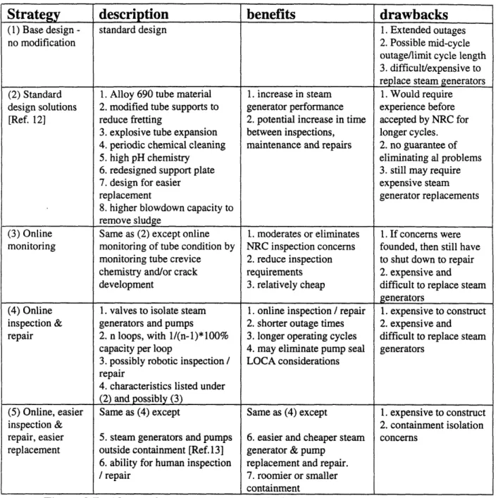
Strategies for redesigning power plant systems were developed. These included designing

plants to allow monitoring, inspection, calibration, maintenance and repair (MICMR) closer

to full power than previously possible (at higher modes of operation); decreasing the time required to perform MICMR, and increasing the times between required MICMR. The

results of the interviews regarding the steam generators were then used in conjunction with

the strategies to illustrate how innovative design solutions can be synthesized from the strategies.

Probabilistic methods for predicting performance of complex systems were reviewed. Monte carlo simulation was chosen as the prefered tool for future research because of its

flexibilities in handling complex, time dependent problems with interdependencies, and

external perturbations. The basis of any redesign of power plant systems should be economics. Therefore, deterministic and statistical cost benefit analysis methods were reviewed.

A simplified simulation model of a pressurized water reactor was constructed, with the feedwater system modelled in greater detail. The model's logic was simplified slightly to

facilitate comparison with an analytical solution to validate the model's structure.

Perturbation calculations were performed on the original model to determine the value of adding redundancy, increasing reliability, and decreasing repair time. It was concluded that

adding redundancy in the feedwater heat exchangers, increased mean time to failure of feedwater components, and decreased mean time to repair of feedwater components

improved capacity factor significantly. This analysis was intended to show how simulation

(3)

3.4.2.5 Unnecessary redundancy 75 3.4.2.6 Complexity 75 3.4.2.7 Dependencies 76 3.4.3 Accessibility 76 3.4.3.1 Inspection 76 3.4.3.2 Maintenance 76 3.4.4 Diversity 76 3.4.5 Architecture 77 3.4.6 Shutdown safety 77 3.4.7 Vulnerabilities to auxiliaries 77 3.5 Economic pressures 77 3.5.1 General comments 77 3.5.1.1 Electricity costs 77 3.5.1.2 Regional effects 77

(9)

3.5.1.3 Breakdown of costs 78 3.5.1.4 Power pools 78 3.5.1.5 Longer cycles 78 3.5.1.6 Plant size 78 3.5.2 Capital costs 78 3.5.2.1 Capital requirements 78 3.5.2.2 Steam generators 78 3.5.3 Capacity factor 79

3.5.3.1 Diminishing returns of longer cycles 79 3.5.3.2 Known costs vs. perceived gains 79

3.5.4 Labor requirements 79

3.6 Operations and maintenance practices 79

3.6.1 Surveillance requirements 80

3.6.1.1 Surveillance interval extensions 80 3.6.1.2 Decreased reliability due to over surveillance 81 3.6.1.3 Staggered vs. sequential testing 81 3.6.1.4 Monitoring vs. physical surveillances 81

3.6.2 Preventive maintenance 82

3.6.2.1 Extending PM periodicities 82

3.6.3 Online testing 82

3.6.3.1 effects of online testing on safety 82

3.6.3.2 effects of longer testing intervals 82

3.6.3.2.1 Setpoint drift

3.6.3.3 Self testing 83

3.6.3.4 Other concerns 83

3.6.4 Predictive techniques 83

3.6.4.1 Maintenance based on predictive techniques 83

3.6.4.2 Monitoring component life 84

3.6.4.3 Specific predictive techniques 84 3.6.4.3.1 Vibration monitoring

3.6.4.3.2 Thermography

3.6.4.3.3 Electrical signatures

3.6.4.3.4 Lube oil testing 3.6.4.3.5 Hydraulic testing 3.6.4.3.6 Leak monitoring 3.6.4.3.7 Batteries

3.6.4.3.8 Performance monitoring

3.6.5 Maintenance policy 85

3.6.6.1 Steaming the plant 85

3.6.6.2 Maintenance philosophies 86 3.6.6.3 24 hour maintenance 86 3.6.5.4 Over maintenance 86 3.6.6 Equipment performance 86 3.6.7 Spare parts 86 3.7 Materials condition 87

(10)

3.7.1 Materials 87

3.7.2 Erosion/corrosion 87

3.7.3 Chemistry of fluids 87

3.8 Cycle length pressures 87

3.8.1 Fuel cycle length 87

3.8.1.1 Plant experience 87

3.8.1.2 Capacity factor arguments 88

3.8.2 Mid-cycle shutdowns 89

3.8.2.1 Required mid-cycle shutdowns 89 3.8.2.2 Economical mid-cycle outages 89 3.8.2.3 Uneconomical mid-cycle outages 90

3.8.3 Refueling outages 90

3.8.3.1 Outage activities 90

3.8.3.2 Reducing outage activities and duration 90

3.8.3.2.1 Critical path activities

3.8.3.2.2 Wet lift system

3.8.3.2.3 Reactor vessel head detensioner 3.8.3.2.4 Spares for quicker maintenance

3.8.3.3 Longer cycles, longer outages 91

3.8.3.4 Staggered outages 91

3.8.4 Forced outages 91

3.9 Advanced technologies 91

3.9.1 Advanced reactor concepts 91

3.9.1.1 Simplification 91 3.9.1.2 Advanced reactors 92 3.9.1.3 Innovative safety 92 3.9.2 Passive systems 92 3.9.2.1 Safety 92 3.9.2.2 Maintenance 92 3.9.2.3 Regulatory risk 92 3.9.3 Digital technology 93 3.9.3.1 Digital circuitry 93

3.9.3.1.1 Capability of digital circuitry

3.9.3.1.2 Effects of radiation on digital systems 3.9.3.1.3 Fiber optic cables

3.9.3.2 Digital controls 93

3.9.3.2.1 Performance of digital control systems 3.9.3.2.2 Regulatory position

3.9.3.2.3 Utility position

3.9.3.2.4 Experience with digital control systems

3.10 Safety 94

3.10. 1 Loss of load events 94

3.10.2 Reactor scrams 95

3.10.3 Interfacing LOCA 95

(11)

3.10.4.1 In favor of using thermal margins 95 3.10.4.2 Opposed to using thermal margins 95

3.10.4.3 Large break LOCA 95

3.10.4.4 Small break LOCA 95

3.10.4.5 Other accidents 95

3.11 Plant size 96

Chapter 4 - Analysis methods 97

4.1 System availability analysis techniques 97

4.1.1. Basic PRA 97

4.1.1.1 The hazard rate (also called the instantaneous

failure rate), X(t) 97

4.1.1.2 The failure rate, f(t) 97

4.1.1.3 The reliability, R(t) 97

4.1.1.4 The cumulative failure probability, F(t) 97

4.1.1.5 Availability, A(t) 98

4.1.1.6 Important failure rate distribution functions 99 4.1.1.6.1 Exponential distribution

4.1.1.3.2 The lognormal distribution

4.1.2 Reliability block diagrams (RBDs) 100

4.1.3 Fault tree / event tree analysis 101

4.1.3.1 Fault trees 101

4.1.3.2 Event trees 101

4.1.3.3 Limitations of fault trees and event trees 101

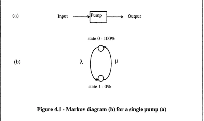
4.1.4 Markov models 101

4.1.4.1 Modelling a simple component 102

4.1.4.1 Limitations of Markov models 103

4.1.5 Direct simulation (monte carlo) 104

4.1.5.1 Setting up the model 104

4.1.5.2 When does simulation become necessary? 106 4.1.5.3 Advantages / disadvantages of Simulation 106

4.1.5.3.1 Advantages 4.1.5.3.2 Disadvantages 4.1.5.3.3 Limitations

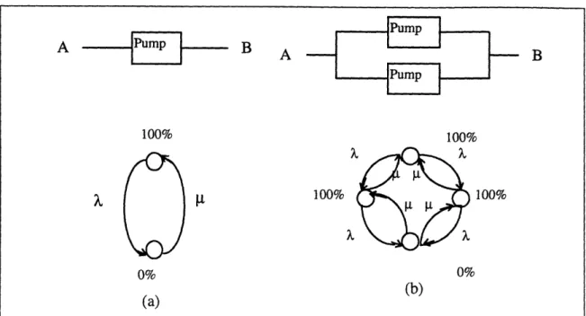
4.1.6 Comparison between Reliabilty block diagrams, Markov

models and simulation for two simple cases 107

4.1.6.1 Example 1 107

4.1.6.1.1 Reliability block diagram analysis

4.1.6.1.2 Markov analysis 4.1.6.1.3 Monte carlo simulation

4.1.6.2 Example 2. 108

4.1.6.2.1 Reliability block diagram analysis

4.1.6.2.2 Markov analysis 4.1.6.2.3 Simulation

(12)

simulation results

4.2 Cost benefit analysis methods 111

4.2.1 Traditional cost benefit analyses 111

4.2.1.1 Example 111

4.2.2 Statistical cost benefit analysis methodology 114

4.2.2.1 A more realistic description of expectations

-probability distributions. 114

4.2.2.2 Probabilistic mathematics 115

4.2.2.2.1 Probabilistic sddition

4.2.2.2.2 Probabilistic multiplication

4.2.2.3 Determining the benefit 115

4.2.2.4 Determining the net benefit 116

4.2.3 Results 117

4.3 Summary 117

Chapter 5 - Analyses 120

5.1 Plant model 120

5.1.1 Block model of a nuclear power plant 120

5.1.1.1 Primary side 120

5.1.1.2 Secondary side 120

5.2 Modeling the feedwater system 123

5.2.1 Failure data 124

5.2.2 Benchmarking the monte carlo plant availability

model against a reliability block diagram analytical solution 127

5.2.2.1 Assumptions 127

5.2.2.2 Success logic 127

5.2.3 Towards a more realistic plant model 128

5.2.4 Perturbations 130

5.2.4.1 Cycle length perturbations 130

5.2.4.2 Effects of redundancy 131

5.2.4.3 Increasing component mean time to shutdown 132

5.2.4.4 MTTR 133 5.3 Summary 134 Chapter 6 - Summary 136 6.1 Interviews 136 6.2 Strategies 136 6.3 PRA methods 136

6.4 Cost benefit methods 137

6.4.1 Deterministic analysis 137 6.4.2 Statistical analysis 137 6.5 Plant model 137 6.5.1 Data 137 6.5.2 Validation 137 6.5.3 Conclusions 138

(13)

6.5.3.1 Cycle length 138

6.5.3.2 Redundancy 138

6.5.3.3 Mean time to failure 138

6.5.3.4 Mean time to repair 138

6.6 Future work 138

6.6.1 Reliability analysis 139

6.6.1.1 Better component reliability and repair data 139

6.6.1.2 Improvements for availability analysis model 139

6.6.1.2.1 High priority items 6.6.1.2.2 Lower priority items

6.6.1.3 Alternate techniques 139

6.6.1.4 Alternate strategy 139

6.6.2 Engineering modifications/ redesign 140 6.6.2.1 Identifying engineering limitations worth further analysis 140

6.6.2.1.1 Identifying poor system performance

6.6.2.1.2 Inspection and surveillance requirements

6.6.2.2 Component specific analyses 140

6.6.2.2.1 Reactor coolant pumps 6.6.2.2.2 Steam generators

6.6.2.3 Predictive monitoring and maintenance 140 6.6.2.4 Online monitoring and testing capabilities 141

6.6.3 Long-lived core design 141

References 142

Appendix A. Simulation program listing in Simscript Language

for base configuration 144

Appendix B. Sample output file from base simulation program 159 Appendix C. Simulation program listing for analytic validation 161 Appenxix D. Mathcad program used in analytic verification of simulation 176

(14)

List of figures

1.1 Maximum theoretical capacity factor 23

1.2 Overall capacity factor as a function of cycle length

and OCF for a 55 day outage length 25

1.3 Research directions 26

2.1 Monitor, inspect, calibrate, mainten and repair at higher

modes of operation - standby safety system as an example 29

2.2 Shorten time to return item to functional state - turbine/generator

as an example 30

2.3 Increase time between shutdowns - turbine/generator as an example 31 2.4 Steam generator inspection, maintenance and repair at higher modes 38

2.5 Shortening steam generator inspection, maintenance and repair 38

2.6 Periodicity of steam generator inspection, maintenance and repair 38 2.7 Alternative steam generator design improvement strategies 41

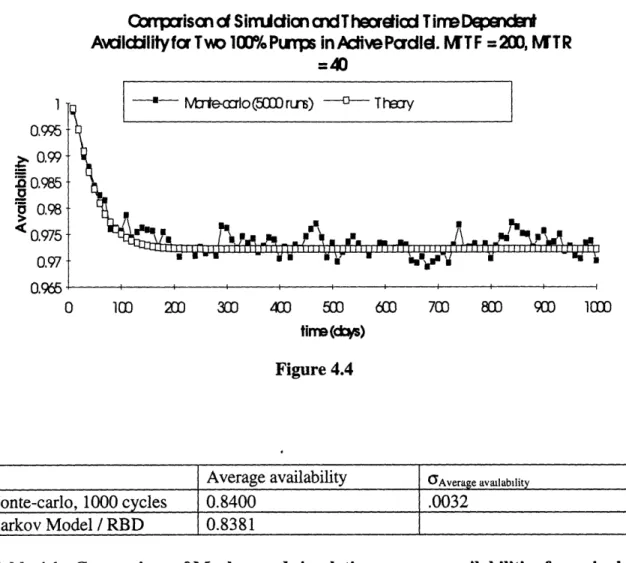
4.1 Markov diagram diagram for a single pump 103 4.2 Markov diagrams for single pump and parallel pump systems 109 4.3 Comparison of simulation and theoretical time dependent availability

for a single pump 109

4.4 Comparison of simulatoin and theoretical time dependent availability

for two 100% pumps in active parallel 110

4.5 Pumping flow diagram 113

4.6 Available pumping systems 113

4.7 Availability distribution for pumping system A 114

4.8 Probabilistic benefit distribution 118

4.9 Probabilistic cost distribution 118

4.10 Cummulative probability distribution for the net benefit of Option 1 119 4.11 Probability density distribution for the net benefit of Option 1 119

5.1 Block diagram model of a PWR 122

5.2 Simplified model of the feedwater system 126

5.3 Comparison of time dependent monte carlo and theoretical

calculations for plant model 128

5.4 Average operational capacity factor vs. operating cycle length 130

5.5 Average capacity factor vs. operating cycle length - 60 day outage 131 5.6 Increase in capacity factor vs. increase in MTTF 133 5.7 Increase in capacity factor vs. increase in MTTR 134

(15)

List of tables

4.1 Comparison of Markov and Simulation average availabilities

for a single pump over a 1000 day period 110

4.2 Comparison of Markov and Simulation average availabilities for

redundant pumps over a 1000 day period. 110

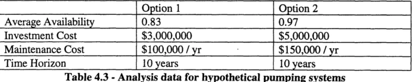
4.3 Analysis data for hypothetical pumping systems 111

4.4 Net benefit matrix 116

5.1 Component reliability data 125

5.2 Success logic for analytical availability analysis 127 5.3 Average availabilities for analytic and simulatoin models over a

1000 day period. 128

5.4 System capacities 129

(16)

Chapter 1- Background. motivation and problem statement

Utilities have long recognized that enhanced economic performance through achievement of improved capacity factor provides an incentive to minimize the duration of refueling

outages. However, because perceived needs for plant shutdown to perform maintenance

and repairs dovetailed with economic optimums for core cycle life, little incentive has existed to run LWRs to cycle lengths longer than 12 to 18 months. Recently however,

some US utilities have extended their operating cycles to 24 months. Nevertheless, this is not a widely accepted strategy nor is it obvious that this length is ambitious enough.

The goal of this project is to examine the strategy of improving capacity factor by

increasing cycle length beyond 24 months. Such an examination entails two facets. First,

the identification of engineering activities necessary to insure reliable operation throughout the duration of the extended operating cycle. Second, the design and economic assessment of cores which can achieve lifetimes consistent with extended cycle length. This project addresses only the first facet. A parallel activity is underway to address the second facet. This project is applicable to both operating and advanced reactor designs. In light of the large amount of activity already expended on core and safety system design of advanced systems, it is likely that the next round of advances in reactor safety and economic performance will be achieved by engineering focus on achieving improved operational reliability. In this regard, examination of gains to be achieved through enhanced

monitoring, inspection, calibration, maintenance and repair (MICMR) activities is strongly

warranted. This project is focused on the development of strategies to improve capacity

factor by achieving reliable, longer operating cycles by enhanced MICMR activities.

This project is also intended to support the work of Hejzlar, Tang, and Mattingly. [Refs. 1,

2 and 3]

The rest of this chapter is intended to provide a background of the current economic

environment in the electric utility industry, and the economic driving factors for nuclear

power in particular.

1.1 Competition

1.1.1 Domestic environment

Historically, US utilities operated as a cost-plus industry. A cost plus environment meant that the investors were assured of a "fair rate of return." All costs incurred by the utility in

operations were covered in the rate base. The investors , however, received an additional return on their capital investments, which was also covered in the rate base. If electrical production costs increased, the utilities appealed to the Public Utility Commission (PUC)

for a rate increase. Under this system, there was little incentive for producing power cheaply, as long as utilities could justify costs to the PUC. [Ref. 4]

(17)

With the passage of the 1992 Energy Policy Act, the United Sates electric utility industry

started down the road to competition. Thus, only recently has widespread competition emerged. Under the new system, utilities are beginning to be required to purchase independent power producers' (IPPs) electricity if it is cheaper than can be produced through the utility. This allows small, non-utility producers to construct cheap, natural gas combined cycle power plants, and undercut the utilities. Fortunately for the utilities, the capacity of the IPPs is still relatively small. Unfortunately, it is growing. Therefore, there is now significant impetus in the United States to make utility produced power cost

competitive.

This is especially true for nuclear power plants. Many of these plants have enormous capital debt, which increases the overall costs associated with nuclear generation.

Compounding that is the historically poor operating performance achieved by these plants

and the high operating and maintenance costs. These components of cost will be discussed

later, but nuclear generating costs are, in general, slightly higher than coal and significantly

higher than natural gas powered electrical generation. The advantage of nuclear power is its

relatively cheap fuel.

1.1.2 International environment

Internationally, nuclear utilities are facing the same pressures. Where available, natural gas fired power plants can produce electricity cheaply and efficiently. Where natural gas is not

plentiful, coal, oil and hydro powered generators are becoming more competitive with nuclear generation. Compounding the economics is the issue of waste disposal. The

United Kingdom has deregulated its utility industry and Japan is proceeding towards

deregulation. Although regulatory structures differ from country to country, in the long

run, cheaper, simpler electric production sources have the potential to overtake the market. Therefore, the problem of nuclear power economics is a global issue, not just a localized

political issue.

1.1.3 Summary

Electric power production is becoming a competitive industry. Worldwide, nuclear utilities

will soon face pressures to become cost competitive. There are several ways to reduce

production costs - each of which will be discussed subsequently. However, if large

generating stations fail to become competitive, they may eventually be forced out of

business.

1.2 The economics of nuclear electricity generation

[Ref. 5] This section is intended to provide an overview of the elements of cost associated with

nuclear power electricity generation. This section will make explicit in a somewhat

simplified fashion the factors that affect nuclear power costs, and will suggest strategies for improving nuclear power economics.

(18)

For any business, net profits are related to revenues and expenses by the following equation:

NP [$] = R- E (1.1)

Where NP [$] = Net Profits R [$] = Revenues E [$] = Expenses

To understand the importance of this simple equation, consider how it affects the overall

costs to consumers. In a competitive industry, the maximum price that utility generated

electricity can be sold at is set by the price (P) of competitor's power expressed in

[$/MWh-e]. If the plant cannot sell power at least as cheaply as its competitor, it cannot sell power. The revenues generated over a given time period are:

R [$] = P * C * Tgen _(1.2)

Where P [$/MWe-h] = Price

C [MWe] = Nominal electric generating capacity Tgen[h] = Generating Time

For a given amount of power produced over a given production time, revenues are fixed. If expenses are greater than revenues, then the plant loses money. This does not mean that it should be shut down, but it certainly means that the expected return to investors is

insufficient. Let us look more deeply into the components of revenues and costs. 1.2.1 Revenues

As mentioned before, revenues are a function of the rate of power production multiplied

by the time this rate of production is maintained multiplied by the mean price received for the power sold. To further decompose it:

R = P * C * (r1 / ) * CF * T (1.3)

where CF = Mean capacity factor

(fl/Tlo) = Thermal efficiency / nominal thermal efficiency

T [h] = Total period of time under consideration

What is seen is that there are a number of ways to increase revenues. The first is to increase the electric power capacity rating of the plant, C. This usually requires

modifications such as revisiting technical specifications, re-doing safety calculations with better analysis tools, and when necessary, modifying plant safety systems to accommodate the power uprating. Therefore, the first assumption made is that this option has been fully

(19)

The second way to increase revenues is to increase the ratio of the average plant thermal efficiency over the period in question to the nominal thermal efficiency over all time

(rl/tl). The reason it fluctuates is that the temperature of the ultimate heat sink varies

from day to day and from season to season. So rq = rl(t), and is out of control of the operator. It is further assumed that the nominal thermal efficiency has been fully maximized.

The third way to increase revenues is to increase average capacity factor. The capacity factor is defined as:

CF = Actual energy produced over a period of time (1.4) Maximum energy that could be produced over that period.

So if a plant ran for 200 effective full power days in the period of 1 year, CF = 200 / 365 = 0.55, or 55%. If the plant were available for 300 EFPDs, the capacity factor would be

82%, and revenues would increase by 50%. Increasing capacity factor will be one of the

main focuses of this thesis.

Finally, for practical purposes, T is merely an accounting tool that sets the period of time over which revenues are to be computed. However, in the long run, T can be used to

represent the design life of the plant. As such, life extension will affect Tma,, - the

maximum operating life of the plant. However, that is beyond the scope of this project.

1.2.2 Expenses

Like revenues, expenses can be further decomposed. Let us look at the various cost components associated with nuclear power, which for present purposes may be

disaggregated as follows:

E [$] = (O&M) + S + F + CP + RC + FF + SR (1.5)

Where O&M [$] = Operations and maintenance costs

S [$] = Salaries

F [$] = Fuel costs

CP [$] = Capital costs

RC [$] = Electrical replacement energy costs

FF [$] = Future expense funds SR [$] = Safety regulation costs

(20)

1.2.2.1 Operations and maintenance costs

Operations and maintenance costs (O&M) are those costs associated with maintaining the

plant material condition and providing operations services.

O&M costs = (M + O) (1.6)

Where M [$] = material condition costs

O [$] = operations services costs

1.2.2.2 Salaries

Salaries (S) are associated with the payment of the workforce necessary to produce and distribute power to the consumer. They are not explicitly included in O&M costs here,

because they are such a dominant cost that they deserve to be considered separately. (In

general, however, discussions of operations and maintenance costs typically include personnel expenses.) The total salary paid is the product of the mean workforce size (which can vary in time due to significant augmentation during refueling outages), the average wage (including overhead and benefits), and the time period in consideration.

S = (CW) * H * T (1.7)

Where (ME) [person] = Mean workforce

H [$/person-h] = Hourly wage

1.2.2.3 Fuel costs

Fuel costs (F) are those costs associated with maintaining the heat source to produce electricity. In standard light water reactors, the fuel costs are a function of unit energy costs (Fc), electrical power capacity (C), thermal efficiency (E), capacity factor (CF) and cycle time (T). In an online refueling scheme, the unit energy costs are constant because enrichment does not need to increase for longer cycles. This is a significant advantage over batch refueling schemes, because in going to longer operating periods in batch schemes,

the enrichment and reactivity control costs can increase significantly.

F = Fc * (C/E) * CF * T (1.8)

(21)

1.2.2.4 Capital costs

Capital costs (CP) are associated with paying back the investors for their initial capital

outlay with a fair rate of return included. It is a function of the plant value (V) and the fraction of the power plant value which is charged as an expense (L) during the time

interval, (T). Here we assume all such costs are levelized over the life of the plant (i.e. charged at an equivalent constant rate).

CP = (V) * L * T (1.9)

Where V [$] L [$/$h]

= Plant value

= Rate of capitalization

1.2.2.5 Replacement power costs

Replacement electrical energy is the cost (RC) of buying more expensive electricity from external sources to replace the power deficit experienced when one of the utility's operating

plants is off-line or at reduced power. It is a function of the average power deficit, the unit

replacement power cost, and the time.

RC = DP) * C * T (1.10)

Where DP [MWe]

Cr [$/MWe]

- average power deficit

= power rating * capacity loss = unit replacement power cost

1.2.2.6 Future expense funds

Future expenses funds (FF) are associated with the costs of plant decommissioning and spent fuel and waste disposal, and time.

FF=(D+W)*T

(1.11)

Where D [$/h]

W [$/h]

= rate of savings for decommissioning = rate of savings for waste disposal

1.2.2.7 Safety regulation costs

Safety regulation is the cost (SR) associated with normal licensing fees and with punitive

actions by the safety regulatory authority. This is a difficult quantity to define or quantify. Nevertheless, it is real and should be included in any discussion of nuclear related costs. It is a function of fines and backfit hardware.

SR =[P, + B] * T (1.12)

Where Pr [$/h] B [$/h]

= Average cost of regulatory fees and fines per unit time = Cost of backfit hardware per unit time

(22)

This concludes the summary of the factors associated with plant expenditures:

Expenses [$] = { (M+S) + C*Fc(CF/ ) + WF*H + V*L + DP*Cr + (1.13)

(D+W) + [Pr+ B]} * T

1.2.3 Net profits, revisited

Combining the results of the previous discussions yields a formula that summarizes the

factors comprising nuclear power economics.

Net Profits [$] = [C * CF * (rl/rlo) * P}- { (M+S) + C*Fc(CF/n) + WF*H + (1.14) V*L + DP*Cr + (D+W) + [Pr + B]}] * T

This research is intended to increase net profits by improving capacity factor. Clearly, capacity factor affects many aspects in the above equation, the most important of which is revenues. The more subtle effects on net profits are increased fuel costs, decreased

replacement power costs, and decreased regulatory costs.

For a continuous refueling scheme, the fuel costs are only a linear function of capacity factor (Revenues Fuel Costs = Constant). In this scheme, going to a longer cycle or a

higher capacity factor does not increase the ratio of revenues to fuel costs. Therefore, the

factors that we will consider in this thesis are (1) increased revenues, (2) decreased

replacement power costs, and to a lesser extent (3) decreased regulatory-associated

availability losses.

For a batch refueling cycle, capacity factor does not greatly affect fuel cycle costs. In reality, current US LWR owners typically plan to run at a high capacity factor between refuelings. If they run very well, they use up all the excess reactivity in the core. If they

do not run well, then they may be forced to "throw out" part of the excess reactivity (i.e. off-load a batch fraction of the core that is not fully utilized). So for a batch cycle, the fuel

costs for a given cycle length are not dramatically affected by an improved capacity factor.

However, increasing the cycle length can significantly increase the unit fuel costs, by increasing uranium ore and enrichment requirements.

1.3 The state of current plants

US PWRs and BWRs had a three year median capacity factor of about 72% for the 1991-1993 period. [Ref.6] In Canada - where refueling outages are not a limitation because of the online refueling capabilities of the CANDU reactors - the three year average capacity factor is around 69%.[Ref. 7] These levels of performance are typical for most operating reactors around the world - with a few notable exceptions that are discussed later. There

are two reasons for this mediocre record. First, when these plants run, they often run

poorly. Maintenance or safety problems force plants to reduce power or shut down frequently. Second, LWRs have to shut down periodically for refueling or major

(23)

surveillances, calibrations, maintenance, and repairs. The duration of these outages vary significantly betwen BWRs and PWRs of various standard designs and between plants of the same standard design operated by different utilities. In the US, they are on the order of

65 days every 18 to 24 months, but range from about 30 days to over 100 days depending on the specific plant.

The two areas of capacity loss suggest three ways to increase capacity. First, decrease major outage durations. Second, increase the period between major outages. Third, improve operational period availability (i.e. reduce forced outages). Figure 1.1 illustrates how shorter outages and less frequent outages affect capacity factors, given perfect

reliability during normal operations (i.e. no forced outages).

Maximum theoretical capacity factor 1 0.98 0.96 0.94 0.92 0.9 0.88 0.86 0.84 0.82 0.8 1 1.5 2 2.5 3 3.5 4 4.5 5

Cycle length [years]

Figure 1.1

Two facts emerge from Figure 1.1. First, if outages can be completed very quickly (say 15

days), there is very little gain from increasing cycle length beyond 12 to 18 months.

Second, if outages cannot be performed very quickly, then significant improvement in

capacity factor can be achieved by extending the cycle length.

1.3.1 Short outage / short cycle strategy

The short outage / short cycle strategy is an approach that Finland has perfected. Finnish outages average 15 days (they actually have alternating 10 and 20 day outages), and they

operate very reliably during the cycle. From the Figure 1.1 we predict that their capacity

factor should approach 96%. In fact, it is around 93%, which is outstanding compared to

world performance. [Ref. 8] There are underlying conditions allowing the Finns to achieve such short outages. First, they have a highly skilled labor force which returns around 90%

of its outage force annually. This assures that outage personnel are familiar with the plant

and require minimal or no training annually. Second, their plants were designed for ease of maintenance. For example, they have extra laydown space, which is at a premium in US

(24)

have outstanding planning. All of these factors allow them to achieve very short, but

highly effective outages. [From interview with Finnish utility representative, coded U27.]

As a counter example to the effectiveness of the short outage, short cycle approach,

consider Japanese outages. Like the Finns, the Japanese are on an annual cycle and run extremely reliably between planned outages. However, the Japanese have very long outages relative to the Finns - around 80 days. This is partially due to regulatory

requirements that force them to do more maintenance than may be necessary on an annual basis. But clearly significant gains in capacity factor could be realized in Japan by

extending cycle length, and keeping the outage duration at 80 days. 1.3.2 Long cycle strategy

For typical major outage times on the order of 55 days or longer, it makes very much

sense to increase the period between major outages to greater than one year, and possibly

up to five years. Note, however, that there is a saturation effect. The gain is very flat past

about three year outage periods. A note of caution about this figure. It is drawn to illustrate how capacity factor changes vs. cycle length for a GIVEN outage duration. In reality, the outage duration may increase (or decrease) as cycle length increases.

Consider the example of Pickering 7 - a CANDU plant owned by Ontario Hydro.

Pickering 7 recently ran for 894 days straight - a new world record.[Ref. 9] This is nearly two and a half years, and is in line with the cycle lengths that should be considered in future designs. The ultimate goal of this line of research is to design a plant capable of

doubling Pickering 7's performance.

1.3.3 Effects of running better during the cycle

Up to this point, the maximum hypothetical capacity factor (MHCF) was considered.

MHCF is the capacity factor the plant would achieve if it ran perfectly during the cycle, and the only down time was due to the planned outage. Let us look at the effect of

improving operating capacity factor (OCF). The operating capacity factor is the capacity

factor achieved by the plant during the cycle. It is defined as the electricity produced during the operating cycle divided by the electricity that could have been produced if the

plant ran at rated capacity 100% of the time during the operating cycle. Figure 2 plots the affect of OCF on overall capacity factor for a 55 day outage, as a function of different

(25)

Overdl cqxcity factor ca afunction of cyde length and OCF for

a55 day outcge length

0.95 0.9 0.9 0.85 0.8 F 0.75 0.7 0.65 n.6 1.5 2 2.5 3 3.5 4 4.5 5 Cydelength (years) Figure 1.2

What Figure 1.2 shows is that it does not matter how long the cycle length is if the plant does not run well during the operational period. A 55 day outage is certainly achievable, even for 2 year cycles. But what is seen in Figure 1.2 is that when the operational availability hovers around 80%, the capacity factor is constrained to 70-75% even for increasing cycle lengths. This confirms the previous hypothesis that improving operational

availability can significantly improve capacity factor and nuclear power economics.

As previously mentioned, reducing outage duration is beyond the scope of this research. Outage management is already being addressed by many experts. However, it is worth

noting that the methods utilized for improving operational availability and increased cycle

length may decrease outage duration. Take the specific example of the Pilgrim nuclear power plant. Pilgrim's critical path item is their ECCS. [Utility representative, coded U19]. Pilgrim has only 2 independent trains, both of which must be maintained during the refueling outage. The ECCS maintenance requirements dictate the length of the outage and the cycle length. By designing for extended cycle length, the capability to surveil, test, and maintain this system online would have to be addressed. As such, this critical path item will be removed from the outage scope, and the outage is free to decrease to the next most limiting challenge. In essence, two difficulties, extended cycle lengths and a critical path outage item, are dealt with by one strategy - online surveillance, testing, and maintenance.

(26)

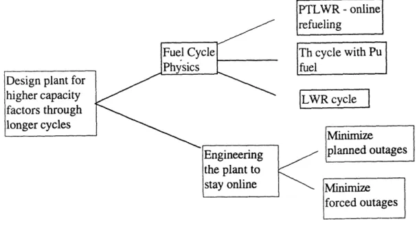
1.4 Research directions

The problems limiting capacity factors have been delineated. The next task is to identify the

areas where research needs to be performed to achieve a higher capacity factor through an

extended operating cycle. As shown in Figure 3, the natural division is between fuel cycle

physics and plant engineering:

IPTLWR - online| eling I :ycle with Pu fR cycle Minimize planned outages IMinimize forced outages

Figure 1.3 - Research directions

This report is concerned with designing the plant to accommodate whichever fuel cycle / reactor combination is chosen. In the subsequent chapters, a strategy is developed to /suggest advantageous system alignments and modifications, and analysis techniques will

be identified and utilized to predict the effects of modifications on plant performance. For now, focus is in the plant engineering direction. It is desired to design power and support systems capable of operating reliably for extended periods of time. Although the specifics

of the fuel cycle and reactor type will affect the design and requirements of certain of plant systems, initial focus will be on those systems common to the different reactor types;

specifically, the power production systems such as feedwater, steam supply, condenser, turbine, reactor coolant pumps, service water, and other continuously operating systems.

(27)

Chapter 2 - Strategy for improving capacity factor

Several areas were identified in Chapter 1 of having potential to increase capacity factor. Those areas were shorter outage duration, longer cycle length, and improved operating

cycle performance. From these broad areas for improvement, several potential strategies emerge which will be discussed in this section.

One of the goals of the plant operator and plant designer is to find ways to minimize unavailability. A general approach to accomplishing this goal is to be able to perform required critical activities (monitoring, inspection, calibration, maintenance, and repair)

* at higher modes of operation (closer to full power)

· quicker

· less frequently.

Modes of operation are generally defined as follows. Mode 1 is defined as power

operation. The plant is typically producing greater than 15% power. Mode 2 is defined as

startup/low power operation. The plant is operating at less than 15% power. Mode 3 is defined as hot standby. The plant is at less than 3% power, but is close to critical. Mode 4 is defined as hot shutdown. The plant is still in hot conditions (between approximately 260 °C and 290 °C for a PWR), but all rods are inserted into the core, and the reactor is subcritical. Mode 5 is defined as cold shutdown. The plant primary temperature is below

approximately 93 °C. Mode 6 is defined as refueling shutdown. The plant primary temperature is below approximately 65 °C, and the primary system is open.

2.1 Moving monitoring, inspection, calibration, maintenance,

and repair to higher modes of operation

The first strategy for improving capacity factor is shortening the amount of time spent out of power production modes. While in lower modes of operation, less or no electrical energy is produced. This reduces revenues and profits, as discussed in Section 1.2. It takes increasing amounts of time to go to and return from progressively lower modes of operation, resulting in additional profit losses.

2.1.1 Power maneuvering

Nuclear power plants can typically change power at a rate of 5% per minute without

exceeding technical specification limits. Therefore, the time loss associated with

maneuvering between power states is small compared to the time required to maintain the

lower power level for monitoring, inspection, calibration, maintenance and/or repair. 2.1.2 Maneuvering between full power and hot shutdown

Although a nuclear power plant can go from full power to hot shutdown in a matter of

(28)

be exceeded, resulting in a safety system actuation. Therefore, it is desirable to approach

shutdown in a controlled manner. As stated, power can be increased or decreased at a rate

of 5% per minute - the plant can go from hot standby to full power in a matter of minutes. In practice, maneuvering plant power is rarely this simple, but as a first approximation, assume that the time required to get between full power and hot shutdown is short.

Therefore, most of the lost electrical generation comes from the time to restore (repair) the plant to its functional state.

2.1.3 Moving from hot shutdown to cold shutdown

The time required to bring the plant from hot shutdown to cold shutdown is not negligible. The maximum primary system heatup and cooldown rates are 100 degrees Fahrenheit per hour. This is set by the thermal stresses put on the reactor vessel. Therefore, it takes a combined minimum of a half a day to cooldown and heat up, ignoring time spent in cold shutdown. In actuality, heatup and cooldown are performed slower than this. Intermediate

states and steps slow the rate at which the reactor approaches power operation. Therefore,

it is assumed that a combined period of at least two days is required to cool the plant down

from power to cold shutdown conditions and then to heat the plant up to return to power

operation.

2.1.4 Moving between cold shutdown and refueling shutdown

In the refueling shutdown condition, the primary system has to be opened. The reactor must be cooled further (typically under 150 °F) and the plant must be put in the refueling shutdown condition. Opening the primary system requires breaking the pressure boundary and requires laborious effort to insure proper controls are observed from a safety and radiological perspective. It is assumed that the additional controls contribute to add a combined week in going into and out of refueling shutdown conditions, starting from cold shutdown.

2.1.5 At power monitoring, inspection, calibration, maintenance, and/or repair

It should be obvious that the value of avoiding lower modes of operation is real and

significant. It was indicated in the industry interviews that if all critical activities could be

performed at power without degrading safety, then capacity factor would be increased substantially. Major outages would be reduced to refueling outages only - a maximum of about 20 days. This may be unrealistic, but the value of online maintenance becomes apparent.

However, industry interviews also expressed some reservations about performing all or

most critical activities at power. Representatives from all backgrounds expressed

reservations over the impacts on safety of performing more activities at full power. For

example, when a system is taken out of service for repair, it is unavailable for safety applications until it is returned to service. If careful consideration is not given, this can increase the overall risk associated with the operation of the plant.

(29)

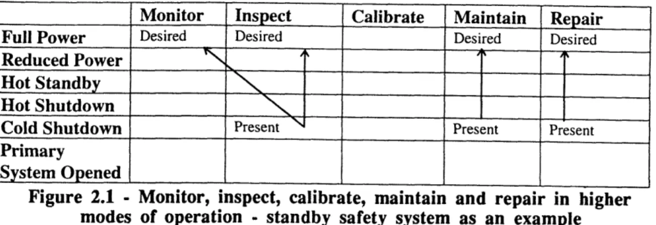
2.1.6 Strategy matrix for monitoring, inspection, calibration, maintenance, and repair at higher modes of operation.

Thus, Figure 2.1 suggests strategies for approaching standby safety system maintenance. The location of the item in the grid shows the typical conditions under which the given operations are currently performed. The arrows signify where it is desirable to perform the given operations. For the specific example of the standby safety system that is inspected at cold shutdown conditions to verify its operability, two strategies are suggested. First, it is desirable to perform the inspections closer to full power. Second, it would also be

advantageous if monitoring could be used to verify the operability in place of inspection, and at higher modes of operation. The matrix also suggests performing maintenance and repair for these systems at higher modes of operation.

Performance of these activities at full power could result in savings in two areas. First, if

safety system inspection, maintenance and repair are critical path outage items, then

performing these activities at power could decrease outage duration. Second, if the standby

safety system limits cycle length, performing these functions at power allow extended

operating cycles without requiring additional costly outages.

Monitor Inspect Calibrate Maintain Repair

Full Power Desired Desired Desired Desired

Reduced Power _____

Hot Standby _

Hot Shutdown

Cold Shutdown Present Present

Primary

System Opened

Figure 2.1 - Monitor, inspect, calibrate, maintain and repair in higher modes of operation - standby safety system as an example

2.2 Shortening repair time (MTTR)

The second strategy involves decreasing the mean time to repair. This applies to

operations, unplanned outages, and major planned outages. The mean time to repair can

also be thought of as the mean time to perform required monitoring, inspections,

calibration, maintenance, and repairs. In short, it is the average amount of time required to

return the entity to the desired state or to verify that the entity is already in the desired state. The time required to repair a component or system directly affects capacity factor. When a

component important to safety fails, the plant is put in a limiting condition for operation. If

that component is not repaired within a specified period of time, the plant will be required

to go to a lower power or a lower mode of operation, resulting in economic losses for the utility. In other cases, a failure may result in an immediate loss of power. In both cases, it is economically advantageous to repair the component or system as fast as possible.

(30)

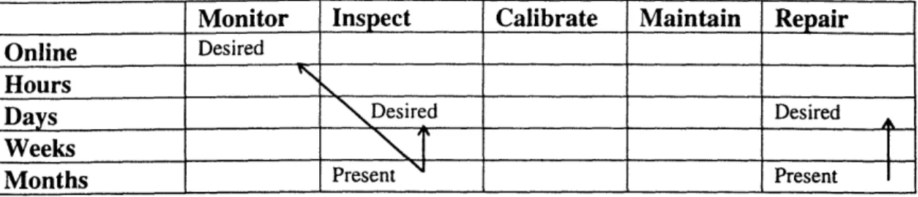
Figure 2.2 illustrates the value of performing required activities quicker. The location of the

item on the grid indicates the approximate duration of time required to return the item to its

functional state. The arrows indicate the direction for improvement.

The example given illustrates that major turbine-generator inspection and repair can take

months. Figure 2.2 suggests that online monitoring may take the place of some

inspections. It shows that investing in better inspection techniques may provide savings. Figure 2.2 also suggests that measures taken to reduce repair times (such as keeping a

spare rotor or spare parts in stock) can be advantageous.

This strategy does not only apply to turbine-generators nor only to monitoring, inspection

and repair. Decreasing the time required to calibrate and maintain components can increase

availability and/or reduce manpower requirements.

Monitor Inspect Calibrate Maintain Repair

Online Desired

Hours

i

Days Desired Desired A

Weeks \ _ _

Months Present Present

Figure 2.2 Shorten time to return item to functional state -turbine/generator as an example

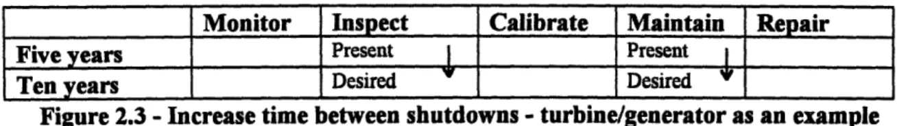
2.3 Extending the periodicity of activities - increasing the mean

time to failure (MTTF)

The final method available to improve plant performance is extending the required

periodicities of monitoring, inspection, calibration, maintenance and/or repair. Mean time to failure is a parameter used to capture all of these activities. Perhaps a better word would be mean time to unavailability or mean time until attention is required. Regardless, if entities can go longer periods before they require attention, then the plant capacity factor will be increased, and cycle lengths can be increased. Therefore, increasing the mean time

to repair of components within plant systems can affect economics.

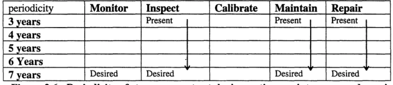
Figure 2.3 suggests increasing the mean time to required attention as a strategy to improve overall reliability. The arrows show the current relation between periodicities of required activities of a given item. The arrow suggest increasing the periodicities. In this example, strategies for increasing the mean time to inspection and maintenance of the low pressure

turbine is examined. Current low pressure turbines require major inspections and

maintenance approximately every five years. The scope of low pressure turbine inspection

and maintenance is enormous, and the time required to perform this is large. Many people

believe that on a five year major outage cycle, if all three low pressure turbines have to be inspected and maintained, turbine maintenance will dictate the length of the outage.

(31)

Therefore, reduction of required low pressure turbine inspections and maintenance is key to longer cycles.

Monitor Inspect Calibrate Maintain Repair

Five years Present I Present

Ten years Desired D' esired _

Figure 2.3 - Increase time between shutdowns - turbine/generator as an example

2.4 Example - Implementation of the strategy to steam generators

The purpose of the following section is to demonstrate by example how the strategies implied by the previous section can be used to help synthesize engineering solutions to real

problems. As discussed in detail in Chapter 3, interviews were conducted with industry representatives to identify issues regarding achieving higher capacity factors through longer operating cycles. One of the sections describing a problematic component identified during the interviews, which fits equally well in Chapter 3, is presented in this section to

illustrate the strategies of Sections 2.1 - 2.3. (Al, A2...; C1, C2...; N1, N2...; P1, P2...; U1, U2...; V1, V2... are codes used to shield the identity of the commentor. Additional codes are used to protect the identity of plants, when disclosure could identify commentor. See Chapter 3 for the key regarding the generic origin of the comment.) Section 2.4

includes the following:

* results of interviews identifying the steam generator as a problem component · discussion of the strategies to be applied to the steam generator

· matrix of proposed design changes based on the strategies.

2.4.1 Interview results regarding steam generators

When asked about the most limiting factors in going to longer cycles or running more reliably, the most popular response - by far - was the steam generators; therefore, steam generator design is an issue worth examining in detail. The most prevalent steam generator

design is the U-tube. For a more detailed description of this device, see [Ref. 10] and [Ref.

11].

The following is a summary of the comments made concerning steam generators during

interviews with representatives from the nuclear industry.

2.4.1.1 Issues/new problems concerning steam generators

2.4.1.1.1 Steam generator tube ruptures

The probability of having a steam generator tube rupture in a PWR is about 0.02 / yr. If the tubes are not inspected or repaired periodically, however, the frequency of tube ruptures may increase. Tube ruptures are currently low contributors to the expected core damage frequency because the plant can usually repressurize, isolate, and shut down

(32)

safely, following a steam generator tube rupture. Nevertheless, tube ruptures are not

insignificant from a safety perspective, and are a serious economic risk. (U20) (U4)

The safety and economic risks from an increased probability of steam generator tube rupture from longer operation and decreased inspections should be analyzed.

2.4.1.1.2 Multiple tube ruptures

There was recently concern that a main steam line break could cause multiple steam

generator tube ruptures due to the degraded states of the tubes and the resultant high pressure drop across them. However, NRC has found that in this event, the pressure drop across the tubes is insufficient to cause multiple ruptures of degraded tubes. (N1)

An analysis by Maine Yankee supports the conclusion that a main steamline break would

not cause multiple tube ruptures. [Ref. 29]

Consequently, multiple degraded tube ruptures due to a main steam line break are not currently limiting, but should be considered for longer cycles.

2.4.1.1.3 Utility perspective

Tube integrity and support plate problems are key to running longer and improving capacity

factor. The advanced reactors have improved materials and chemistry; have reduced hot leg temperature; and have incorporated past experience. The performance of replacement steam

generators should give some indication of how redesigned steam generators may perform in the future. (P4)

Steam generator tube leaks are also a big concern to utilities, and may be the limiting factor

in going to longer cycles. If tubes are not inspected periodically, there may be a tube rupture, and this can have serious impacts on capacity factor and operations. (C2) (Ul 11) (C4) (U4)

2.4.1.1.4 Regulatory perspective

Steam generator tubes are a limiting problem in extending cycle lengths. NRC would be skeptical of running a plant five years without inspections, even if all of the problems were believed fixed. The NRCs position is that the utilities might as well plan on having

problems with the steam generators. (V2) (N2)

If a plant has a problem steam generator or if there are indications of degradation, then there

may be a regulatory requirement to inspect and plug or sleeve tubes on a specific schedule

that is less than the cycle length. If there is a history of leakage, NRC isn't going to permit longer operating cycles without inspections. (V2)

2.4.1.1.5 New problems

There are new tube degradation mechanisms being discovered all the time (every 5 years or so). PWR_#6 and another plant recently had tube ruptures between the support plate, which is a new problem. (C4) (N2)

(33)

2.4.1.1.6 Aging

Steam generator degradation is a function of the age of the generator. There has to be

sleeving and plugging done to maintain the primary system's integrity. (U20) 2.4.1.1.7 Planning for problems

Significant savings could be achieved by planning to replace the steam generators in the design phase. Maintenance capabilities should be considered when designing the steam generator. (N1) (V1)

2.4.1.2 Steam generator redundancy and loop isolation valves 2.4.1.2.1 Redundant loops for online work

Redundancy can be designed into the steam generators. Loop stop valves can be used to

isolate one loop of the reactor coolant system to allow inspections, maintenance and

repairs while the rest of the plant is at power. The design would be for N-1 loop

operation - four 33% capacity loops, five 25% capacity loops, etc. This is advantageous because it is not necessary to shut down the plant and open the primary system when a tube leaks or to do required inspections and maintenance. The Russians have 6 loops, and may have done this. It probably wouldn't make sense to have a design where power would

have to be reduced to do the inspections and maintenance, because the economic incentive

is lost. (Ul 1) (C4) (V2) (C2)

The downside to designing to isolate and drain one loop during operation is that

complexity and maintenance burden are increased. There are now more tubes, pumps, and

valves to fail and maintain. Further, the additional complexity translates into additional

costs. It is expensive to add an extra loop or extra capacity. (P3) (C2) (U11)

2.4.1.2.2 Safety issues associated with online work

The capability to use valves to isolate a reactor coolant system loop is not out of the

question. The Navy has loop stop valves, and the NRC staff has accepted them. They can be made reliable enough to prevent an accidental LOCA. (N2)

However, if it is desired to do online loop maintenance, multiple valves become necessary

to prevent a large LOCA and for safety of personnel. If there are two valves is series, they can be tested for leakage by measuring the pressure between them.

From a maintenance perspective, personnel are in containment with the potential for an

accident, so it may not be safe for the workers, and it also raises containment isolation

questions. (U20)

2.4.1.2.3 Shutdown maintenance

Having isolation valves is also a good way to isolate the steam generators after shutdown.

Isolation valves eliminate the need to construct nozzle dams to keep water out of the steam generators. Nozzle dams tend to leak and they are not designed to withstand much

(34)

pressure. If there is any sort of pressure transient, the dam will leak or fail. With isolation valves the steam generators can be accessed earlier in an outage, with less probability of

leakage. (V2) (U13)

Loop stop valves are desirable for steam generator maintenance because the plant does not have to go to mid-loop as often as in other plants. Mid-loop operation is a very risky condition because there is so little water inventory. (U13)

2.4.1.2.4 Stop valves under tube rupture conditions

PWR_#2 has loop stop valves, but in the event of a tube rupture, the plant has to equalize the pressure between the primary and the secondary before it can be ensured that the valves

will close. PWR_#2's stop valves do not work well under high differential pressures. The

stop valves are not in any of the emergency operating procedures or any accident

sequences. (U20)

2.4.1.3 Materials and specifications

2.4.1.3.1 Material selection

Better alloys need to be chosen for the steam generator tubes. The new steam generators use Inconel 690, which has been shown to be a lot better than the old steam generator

tubes, but NRC will not allow five years of operation without inspecting the tubes. Surrey and Turkey Point should have good data on Inconel 690 performance. Inconel 690 is

probably the best material available, but materials selection is still somewhat of an art-form. It may be advantageous to look at exotic materials for the tubes. Exotic materials may be

much more expensive initially, but these materials would pay off in the long run.(U12)

(U24) (C4) (V2)

2.4.1.3.2 Materials specifications I fabrication

In addition to material types, the specifications for the tubes are important. Excellent

quality control (QC) over the fabrication of materials is absolutely necessary. Good construction techniques are also important. Full length tube expansion and the use of explosive expansion of the tubes in the tubesheet is superior to rolling the tubes and older techniques. The tubes should not be rolled because rolling leaves residual stresses and makes stress corrosion cracking a possibility. An important specification is the acceptable level of residual stresses. (U24) (V1) (U12)

2.4.1.3.3 Secondary side factors

Key elements to steam generator performance include not only good steam generator materials selection, but also secondary materials selection. The secondary system

chemistry dictates the performance of the steam generators. A condenser with no in-leakage of brackish water is important so titanium condenser tubes should be used to avoid tube failures. Feedtrain materials selection is important, and copper and catalysts should be avoided. Finally, things like resin beads must be prevented from getting to the condenser.