Upper bound computation for buffer backlog on AFDX networks with multiple priority virtual links

HAL Id: hal-02348192

https://hal.archives-ouvertes.fr/hal-02348192

Submitted on 5 Nov 2019

HAL is a multi-disciplinary open access

archive for the deposit and dissemination of

sci-entific research documents, whether they are

pub-lished or not. The documents may come from

teaching and research institutions in France or

abroad, or from public or private research centers.

L’archive ouverte pluridisciplinaire HAL, est

destinée au dépôt et à la diffusion de documents

scientifiques de niveau recherche, publiés ou non,

émanant des établissements d’enseignement et de

recherche français ou étrangers, des laboratoires

publics ou privés.

Upper bound computation for buffer backlog on AFDX

networks with multiple priority virtual links

Rodrigo Coelho, Gerhard Fohler, Jean-Luc Scharbarg

To cite this version:

Rodrigo Coelho, Gerhard Fohler, Jean-Luc Scharbarg. Upper bound computation for buffer backlog on

AFDX networks with multiple priority virtual links. Annual ACM Symposium on Applied Computing

(SAC 2017), Apr 2017, Marrakech, Morocco. pp.586-593. �hal-02348192�

Any correspondence concerning this service should be sent

to the repository administrator: [email protected]

This is an author’s version published in:

http://oatao.univ-toulouse.fr/22332

Official URL

DOI : https://doi.org/10.1145/3019612.3019729

Open Archive Toulouse Archive Ouverte

OATAO is an open access repository that collects the work of Toulouse

researchers and makes it freely available over the web where possible

To cite this version:

Coelho, Rodrigo and Fohler, Gerhard and

Scharbarg, Jean-Luc Upper bound computation for buffer backlog on

AFDX networks with multiple priority virtual links. (2017) In: Annual

ACM Symposium on Applied Computing (SAC 2017), 4 April 2017 - 6

April 2017 (Marrakech, Morocco).

Upper Bound Computation for Buffer Backlog on

AFDX Networks with Multiple Priority Virtual Links

Rodrigo Coelho

Gerhard Fohler

Jean-Luc Scharbarg

ABSTRACT

In recent avionics systems, AFDX (Avionics Full Duplex Switched Ethernet) is the network used to replace the previ-ously deployed point-to-point networks. In AFDX networks, nodes are not synchronized and therefore data contention re-peatedly occurs at the switches output ports. AFDX switches implement output buffers on each output port to address the data contention issue. Considering the safety critical appli-cation of AFDX networks, overflow of these buffers must be avoided at all cost to prevent data loss.

In this paper we consider AFDX networks that allow for the classification of traffic into more than two priority levels. We present a novel method to compute an upper bound for the backlog of each priority buffer of each output port on a AFDX network with multiple priority traffic.

Keywords

Networks, buffer backlog, upper bound, AFDX network

1.

INTRODUCTION

Avionics full duplex switched Ethernet (AFDX), standard-ized as ARINC 664-P7 [1], is an Ethernet based network tai-lored to account for avionics constraints. Avionics functions are distributed on a set of end systems (ES) interconnected by an AFDX network. Each ES is connected to exactly one switch port and each switch port is connected to at most one ES. AFDX switches relay all ingress frames according to the store and forward paradigm.

DOI:http://dx.doi.org/10.1145/3019612.3019729

End systems exchange frames through virtual links (VLs). A VL statically defines a unidirectional virtual communication channel between one source ES and one or more destination ESs. A bandwidth allocation gap (BAG), a minimum and a maximum frame length (Sminand Smax) and a priority level define the properties of a VL. The BAG defines the minimum time between the transmission of two consecutive frames of the associated VL: consequently, we can classify a VL as a sporadic flow. The path of each virtual link is fixed and de-fined at design time. The current ARINC 664-P7 standard defines two priority levels for VLs. However, some commer-cial AFDX products allow for the assignment of multiple priority levels to VLs. For instance, the AFDX switch pre-sented in [10], permits the classification of virtual links with 8 priorities, allowing the generation of a non-preemptive rate monotonic frame schedule.

AFDX end systems do not share any notion of global time and consequently are not synchronized. Thus, frames that ingress a switch from separate physical links might compete for the same output port at the same moment in time, lead-ing to data contention. AFDX resolves this data contention issue by means of buffering [1]. Due to the safety criti-cal requirements of avionics systems, buffer overflow and the resulting data loss must be avoided at all cost. There-fore, the network designer must reserve enough memory for each buffer so that they do not overflow at run time. Over-reservation, however, has to be avoided. Due to the non synchronized dispatch of frames, obtaining the largest buffer backlog by simulating all possible combinations of frame ar-rivals is intractable for an industrial AFDX network. We consider, in this work, a AFDX network with multiple priority traffic and present a method to compute an upper bound for the backlog of each buffer on the network. The main contribution of this paper is twofold: first, present-ing the arrival order of the frames that leads to the largest backlog (worst case scenario) for each priority buffer on each output port of each switch; second, present the equations to compute an upper bound for this backlog, providing a method to dimension AFDX buffers for multiple priority traffic.

This paper focuses on the worst case analysis, the respective proofs, and equations for the upper bound computation. We defer to a future work the comparison between the upper bounds achieved with the method presented in this paper against those achieved by other existing methods.

The paper is organized as follows: Section 2 presents the related work; Section 3 presents the assumptions, notations and definitions used in this paper; Section 4 presents an overview of our method; Sections 5 presents the worst case scenario and the upper bound computation for the buffer backlog of AFDX networks with multiple priority traffic; Section 6 discusses the applicability of our method in switches with assumptions different from those used in this paper; and Section 7 presents the conclusions and future work.

2.

RELATED WORK

Several methods have been presented to compute an upper bound for the buffer backlog of AFDX networks under differ-ent assumptions. Next we presdiffer-ent the related work grouped by the number of addressed priorities.

Single priority traffic: [2] presents a method to provide the exact analysis of AFDX networks and the respective computation of exact end-to-end delays. This method how-ever does not scale and consequently can not be used in industrial AFDX networks with hundreds or thousands of virtual links. [3] computes backlog upper bounds using the trajectory approach (TA). The authors show that for the majority of the investigated case, TA leads to bounds tighter than network calculus (NC). [8] shows that the end-to-end delay bounds (and possibly the buffer backlog upper bound) computed by the trajectory approach can be optimistic in some cases and identifies the source of the optimism. This problem was addressed by [9]. Most recently, [7] presented the forward end-to-end delay approach (FA) which computes an upper bound for the end-to-end delay for AFDX networks based on the maximum backlog of single priority traffic. As an intermediate result of the end-to-end delay, FA computes the largest buffer backlog for each output port.

Two priorities traffic: Results on the upper bound for the buffer backlog of AFDX networks with two priority traffic have been presented in [6]. However, some of the conditions assumed for the worst case scenario are not realistic, e.g. frames arriving in decreasing order of size per priority level independent of their virtual links.

Many priorities traffic: [3] uses network calculus to com-pute stochastic upper bounds for multiple priority traffic. The authors consider that the system interconnected with the AFDX network can handle buffer overflow and assume that applications are designed to give accurate results even if they miss some frames. [4] presents the computation for the buffer backlog upper bound of AFDX networks under the unrealistic assumption that all frames have the same size. In comparison to previous work, our paper computes a deter-ministic, i.e. not stochastic, upper bound for the backlog of each priority buffer of each output port on a AFDX network with multiple priority levels traffic. Our solution further relaxes the unrealistic assumption that all frames have the same size.

3.

ASSUMPTIONS, NOTATIONS AND

DEF-INITIONS

This paper assumes an AFDX network N comprised of a set of AFDX nodes, i.e. end-systems and switches as

de-scribed in the AFDX standard [1], a given network topology, a network bandwidth BW constant and equal for all physical links, a set of virtual links and fixed paths for each virtual link. Further, this paper assumes:

• each virtual link is classified with one out of a set of priority levels (one, two or more priority levels) • the network switches apply the fixed priority first-in

first-out (FP/FIFO) algorithm to dispatch the ingress frames to the respective output ports

• switches dispatch ingress frames according to the store and forward paradigm, i.e. a frame can only be trans-mitted after it is completely stored in the output buffer • data transfer occurs bit-wise, i.e. frames are copied to and removed from the output buffers bit by bit, respectively as frames ingress or egress

• the path of each virtual link is known

• each output port of each switch has one buffer for each priority level.

Additionally, this paper assumes that there exist a method that provides the frames in the largest busy period encoun-tered by a frame of each virtual link. The trajectory ap-proach, for instance, is one possible method. Notice that any other method that computes the number of competing frames can be used in our approach.

This paper uses the terminology time of transmission and time of arrival to refer to the time when a frame is com-pletely transmitted and received, respectively. Further, the terms ingress and arrival of frames, and egress and trans-mission of frames are used interchangeably. We use the term competing frames to refer to all frames present in the busy period of the virtual link under analysis and scenario to refer to a specific arrival sequence of competing frames. We consider that each full-duplex connection (link) between two nodes in the network is seen by each node as two unidi-rectional links: one input and one output link.

Table 1 presents the terms, indices and sets used to describe and to compute the upper bound for the buffer backlog in each buffer of each switch on an AFDX network.

We summarize the meaning of three functions presented in Table 1 as follows: s(fa_{) computes the size of a given frame} fa_{; t(s(f}a_{)) computes the time required to transmit this} frame; d(time) is the inverse function of t(size), i.e. com-putes the amount of data transmitted during a given interval of time. One can compute the data transmitted during the transmission time of fa_{as d(t(s(f}a_{))), which is equivalent to} s(fa_{). Notice that, different from s(), d() takes a time value} as an input. In this paper, the positive part of any variable is represented with the notation ()+, e.g. (∆)+= max(0, ∆).

4.

OVERVIEW

Algorithm 1 presents an overview of the steps used in our method to compute an upper bound for the buffer backlog on the output ports of AFDX nodes. In order to compute an upper bound for the backlog of a buffer on the network (for each output port o – Line 1, one buffer per priority p – Line 2), we compute the competing frames (Line 4) of each egress virtual link v (Line 3) with the same priority as

Table 1: Notations

N AFDX network, i.e. switches, end-systems, net-work topology and virtual links (including their routes)

BW Network bandwidth

O Set of output ports in the network

o, p, i, v Indices used to represent a switch output port, priority, input link and a virtual link, respectively CFv,o _{Set of frames that compose the busy period of a}

frame of the virtual link v on the output port o. Po _{Set of priorities of all VLs that egress the output}

port o (same port as virtual link v )

Io _{Set of input links connected to the same switch}

as the output port o

Vo,p _{Set of virtual links of priority p that egress the}

output port o

Vo,p,i _{Set of virtual links of priority p that egress the}

output port o and ingress from the input link i * Index and acronym used to represent the scenario

leading to the largest backlog faced by a virtual link (worst case scenario)

’ Index and acronym used to represent a scenario other than the worst case scenario

ω Time when the first frame starts to arrive in the scenario under analysis

α Time when the first frame starts transmission in the scenario under analysis

β Time when the latest frame of priority other than the frame under analysis completes transmission θp _{Time when the latest frame of the priority under}

analysis or of higher priority arrives s(data) Function that computes the size of data t(size) Function that computes the time required to

transmit some data of length equals to size over a physical link, i.e. t(size) = size/BW

d(time) Function that computes the maximum amount of data transmitted on a physical link during a time length equal to time, i.e. d(time) = time ∗ BW σpALL Sum of the size of all frames with priority p

σp_Interval Sum of the size of frames with priority p trans-mitted during a given interval

R*p_(b−a) Amount of received(R) data of priority p in sce-nario * during the interval ]a, b]. T_(b−a)*p repre-sents the respective amount of transmitted data P-buffer,

P-frame, P-data

Respectively, buffer, frame and data of priority p

Bθ*pp P-buffer backlog at time θ*p in the worst case

scenario

Bo,p,v,max _{Largest P-buffer backlog perceived by a frame of}

the virtual link v

Bo,p,max _{Largest P-buffer backlog, i.e. after considering all}

priority p virtual links

blp_{(t) Function to compute P-buffer backlog at time t}

δR’pτ The difference on the amount of data that ingress

from ω*_{until τ between the scenario ’ and *. δT}’p τ

is the counterpart for egress frames

the buffer under analysis. Then, we compute in Line 5, the largest backlog encountered by a frame of this virtual link. In Line 7, we calculate the upper bound for the backlog of the buffer of priority p by computing the largest backlog among all virtual links of priority p that egress the output port o.

Algorithm 1 Upper bound computation overview 1: for each output port o ∈ O do

2: for each priority p ∈ Po _do 3: for each virtual link v ∈ Vo,p _do

4: CFv,o _{= GetCompetingFrames(N, o, v)} 5: Bo,p,v,max= ComputeBacklog(CFv,o₎ 6: end for 7: Bo,p,max= max ∀v∈Vo,p(B o,p,v,max ) 8: end for 9: end for

In order to improve readability, the next sections omit the output port index o whenever possible.

4.1

Intervals

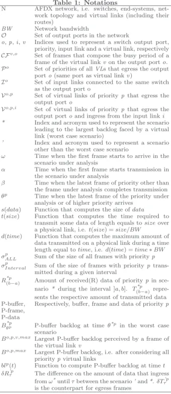
For the analysis of the buffer backlog of any given priority, e.g. P, we investigate the transmission and reception of P-frames during time intervals classified according to Table 2. This table presents the buffer backlog accrual according to the reception and transmission of P-frames as well as to the size of the respective interval. It is noteworthy that any time interval that does not match the properties of Table 2 can be decomposed into smaller intervals until each of them adheres to properties of an interval type presented in Table 2. Table 2: Interval types description and respective buffer backlog accrual

interval type ingress of P-frames egress of P-frames backlog accrual 1 Yes No σP Interval 2 Yes Yes σP Interval−s(Interval) 3 No No 0 4 No Yes < 0

In intervals of type 1, P-frames ingress and no P-frame egresses during the whole interval. Consequently, the back-log accrual is equal to the sum of all data that ingress P-buffer in this interval. In intervals of type 2, P-frames ingress and egress during the complete interval. Consequently, the backlog accrual is equal to the sum of all P-data that ingress P-buffer minus the length of the interval. In intervals of type 3, no P-frame ingresses or egresses the buffer and con-sequently the P-buffer backlog does not change. In intervals of type 4, no P-frame ingresses while P-frames egress during the complete interval. Thus, the backlog decreases during type 4 intervals.

The example in Figure 1 depicts all types of intervals. The upper part of the figure presents the ingress competing frames on the input links IL1 to IL4 and the egress frames on the output link (OL). The central part of Figure 1 presents the backlog on P-buffer and lower part the intervals types. Next, we present the important points in time used for the backlog computation of the P-buffer backlog. Notice that the scenario index (*, ’ ) is omitted since the following ex-planations apply for any scenario.

P-buffer bac klog OL IL 1 IL 2 IL 3 IL 4 ω′ α′ θ′p t frames hp p lp 1 2 3 4 in terv al typ e

Figure 1: Example scenario. Ingress and egress frames at the top, buffer backlog as a function of time in the middle and interval types at the bottom

• ω: start of arrival of the first ingress frame • α: start of transmission of the first egress frame • β: time when the latest frame of priority other than

the one under analysis completes transmission • θp_{: time when the latest frame of the priority under}

analysis or of higher priority arrives

For the sake of simplicity and without loss of generality, we assume in this paper that the start of arrival of the first ingress frame occurs at t = 0, i.e. ω = 0.

Additionally, we define a new variable ∆ to represent the amount of transmitted data between θp _{and β, i.e. ∆ =} d(θp_{− β). Negative values of ∆ are analyzed separately and} reflect scenarios in which the latest frame of priority other than P egress after the ingress of the latest P-frame.

5.

BUFFER BACKLOG UPPER BOUND

FOR MANY PRIORITIES TRAFFIC

We divide this section into three parts: the first part presents the scenario leading to the largest backlog (worst case sce-nario); the second presents the computation of the buffer backlog upper bound encountered by a frame of the virtual link under analysis; and the third presents the backlog upper bound computation for the buffer under analysis.

We assume that each virtual link is classified with one pri-ority (P) out of a set of many priorities, not only two. For the analysis of the backlog of the P-buffer encountered by a virtual link v on a output port o, we classify each virtual link that egresses this output port into: HP, LP or P to re-fer to the virtual links with higher, lower priority or same priority than the virtual link under analysis, respectively.

5.1

Worst Case Scenario

This section starts presenting a formal description of the worst case scenario and the respective proofs. Then, we present the computation of the important points in time used in the computation of the buffer backlog upper bound. This section concludes describing the impact on the upper

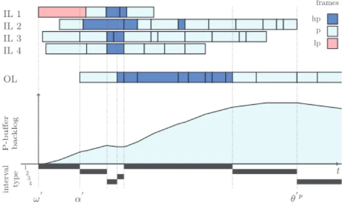
P-buffer bac klog OL IL 1 IL 2 IL 3 IL 4 ω∗ _α∗ _β∗ _θ∗p t frames hp p lp 1 2 3 4 in terv al typ e

Figure 2: Worst-case scenario for P-buffer consider-ing the same competconsider-ing frames of Figure 1

bound computation due to some mutually exclusive condi-tions assumed in the description of the worst case scenario. Figure 2 depicts the worst case scenario (index * ) for the P-buffer backlog with the same competing frames of Figure 1. Theorem 1 describes the properties of the worst case scenario for the P-buffer backlog.

Theorem 1. The scenario leading to the largest backlog encountered by a frame of a virtual link of priority P presents the following properties: i) the smallest sum of lengths of type 2 intervals, ii) no type 4 interval before the arrival of the latest P-frame, iii) no type 2 interval before the latest type 1 interval, and iv) the largest P-buffer backlog occurs at the point in time when the latest P-frame arrives, i.e. θ*p_. Next, we prove the four properties of Theorem 1.

i) Smallest sum of lengths of type 2 intervals Proof. _{The backlog at θ}*p _{is equal to the sum of all} ingress P-data minus the sum of all egress P-data until θ*p_. Considering that no type 4 interval occurs before θ*p_, P-data can only egress during type 2 intervals, therefore the backlog at θ*p_{is equal to:}

B*p θ*p= σ p ALL− X s(Intervaltype2)

Consequently, the shorter the sum of lengths of type 2 in-tervals, the larger the P-buffer backlog at θ*p. Thus, in the worst case scenario, the shortest sum of lengths of type 2 intervals occurs.

ii) No type 4 interval occurs before the arrival of the latest P-frame

Proof. _{During intervals of type 4 the amount of data} in the P-buffer decreases (see Section 4). Consequently, in the worst case scenario no interval of type 4 occurs until the last P-frame arrives.

iii) No type 2 interval occurs before the latest type 1 interval

Proof. Let β’_{represent the transmission time of the last} frame of priority other than P in a scenario different than

the one described in Theorem 1, i.e. the counterpart of β*_. We compare the buffer backlog in two different scenarios: the scenario described by Theorem 1 and another scenario in which P-frames are transmitted before β’_{. We prove that} there exists no scenario in which the buffer backlog is larger than the backlog at θ*p in a scenario described by Theo-rem 1.

Let B’p

τ be the buffer backlog of scenario ’ at a given moment in time τ and Bτ*pbe the buffer backlog of scenario * at the same time τ . We prove that B’p

τ at any point in time is not larger than the buffer backlog at θ*p _{in the worst case} scenario.

The buffer backlog of scenario ’ at any point in time τ is equal to the buffer backlog of scenario * at the same time τ plus the difference (increase or decrease) of the amount of data that ingresses minus the difference on the amount of data that egresses P-buffer from ω* _{until τ . We assume} ω*= 0, and represent B’p τ as: Bτ’p= Bτ*p+ δR’pτ − δTτ’p (1) where δR’pτ = R’pτ − R*pτ (2) δTτ’p= Tτ’p− Tτ*p (3) In the worst case scenario, we represent the backlog at θ*p w.r.t. any point in time τ as:

B*p_θ*p=B*pτ + R_(θ*p*p_−τ)− T_(θ*p*p_−τ) (4) Consequently, from Equation (1) and (4) we represent the difference between B*p_θ*p and Bτ’pas:

B*p θ*p− Bτ’p=R*p_(θ*p−τ)− T *p (θ*p−τ)− δR ’p τ + δTτ’p Considering that, per definition R(a−b)= Ra− Rb, then:

R*p

(θ*p_−τ)= R*pθ*p− R*pτ = σ p

ALL− R*pτ σp_ALL= R’pτ + R’p_(θ’p_−τ)

After some algebraic manipulation we have: B*p θ*p− Bτ’p=R’p_(θ’p−τ)− (T *p (θ*p−τ)− δT ’p τ ) (5) We prove, in the Appendix, that Equation (5) is larger than or equal to zero for any value of time τ .

iv) The largest P-buffer backlog occurs at θ*p Proof. _{According to Theorem 1, in the worst case} sce-nario no type 4 interval occurs before θ*p_{, i.e. the backlog} on the P-buffer does not decrease until θ*p_{. Therefore, the} value of the P-buffer backlog can be represented by an in-creasing function blp_{(t) where t varies from ω}*_{until θ}*p_and consequently: blp_(θ*p_{) ≥ bl}p_{(τ ), ∀ ω}*_{≤ τ ≤ θ}*p

5.1.1

Computation of

According to Theorem 1, in the worst case scenario, no in-terval of type 2 or 4 occurs before β*_{and no P-frame arrives} after θ*p_{. Consequently, in the worst case scenario, intervals}

of type 2 may only occur between β* _{and θ}*p_{. Thus, the} sum of the lengths of type 2 intervals is limited by θ*p− β*. Therefore, the smallest sum of lengths of type 2 intervals requires the largest β* _{and the shortest θ}*p_.

The largest β*implies the largest amount of time, after ω*, in which no P-frame is transmitted. Three effects may delay the transmission of P-frames and define the value β*_{: idle} time, blocking and interference.

The store and forward characteristic of AFDX switches leads to idle time during the arrival of the first competing frame. This idle time, in turn, delays the transmission of all com-peting frames. Blocking and interference occur when the delay on the transmission of a frame is caused by frames of lower and higher priority, respectively.

In the worst case scenario, the largest sum of those effects occur and results in the value for β*_:

β*= max idlev+ max interfv+ max blockv (6) Because of the initial idle time caused by store and forward, the larger the first ingress frame, the larger the initial idle time (and consequently the larger α*_{). [3] has proven that} there exists no scenario in which the sum of idle times on the output link is larger than the length of the largest frame (assuming no idle time on the input links). Therefore, the largest idle time occurs when the first arriving frame is the largest (see Figure 2 from ω* _{until α}*_{), i.e.:}

max idlev= α*= t(s(fmax)) (7) The largest possible interference occurs when all HP-frames delay the transmission of P-frames stored in the P-buffer. Therefore, in the worst case scenario, all HP-frames arrive from their respective input links and are transmitted before the first P-frame starts transmission. Equation 8 computes the maximum interference.

max interfv= t(σALLhp ) (8) To ensure that no P-frame is transmitted before β*_{, we} assume that the largest HP-frame is the first transmitted frame.

Two categories of frames might be blocked: HP-frames (by LP-frames and P-frames) and P-frames (by LP-frames). Nev-ertheless, in the worst case scenario, we account for block-ing caused only by LP-frames. For a P-frame to block a HP-frame, this P-frame must arrive before the transmission of the HP-frame, and consequently, before β*. However, no P-frame is transmitted before β* _{(Theorem 1 properties ii} and iii ) and consequently not before the latest HP-frame. Therefore, we do not consider the blocking caused by P-frames.

A LP-frame can only egress when no P-frame or HP-frame is stored in their respective buffers at the moment when the output port is not transmitting any frame. Blocking oc-curs when a P-frame or a HP-frame is completely stored in its respective buffer while the LP-frame egresses, i.e. if an LP-frame is the first arriving frame and starts transmission just before the complete arrival of the blocked frame. In the worst case scenario, the largest LP-frame is the first arriving frame and the blocked frame arrives a short amount of time

(ǫ) later. The impact of both blocking and interference on the analysis of the P-buffer backlog is the same: they post-pone the transmission of P-frames and consequently lead to an increase on the backlog in the P-buffer. Therefore, we assume that in the worst case scenario, the transmission of the first HP-frame is blocked by the largest P-frame, which in turn delays the start of the transmission of P-frames (see Figure 2). Equation (9) computes the largest blocking time: max blockv= t(s(flp,max)) (9) For the analysis of virtual links with the highest priority among all competing frames, no HP-frames exists and con-sequently max interfv = 0. Similarly, for the analysis of virtual links with the lowest priority among all competing frames, no LP-frames exists and consequently max blockv = 0.

In order to compute the smallest value for θ*p_{, we define θ}*p i as the arrival time of the latest P-frame of each input link i. Consequently, the arrival time of the last P-frame among all input links is:

θ*p= max ∀¯i∈Ioθ

*p ¯i

We use the term “sequence” (seqi) to define the set of com-peting frames that ingress from the same input link i. Equa-tion (10) computes the size of a sequence:

s(seqi) =

X ∀fk_∈CF¯v,o_,∀¯v∈Vo,p,i

∀¯p∈Po

s(fk) (10)

For a scenario with no idle time on the input links, Equa-tion (11) computes the arrival time of the last frame on an input link (θ*pi ) by adding the size of the sequence on this input link (s(seqi)) to time when the first frame of this input link (f1

i) starts transmission (s(gapi)):

θi*p= t(s(gapi) + s(seqi)) (11) According to Equation (11), the only term on the compu-tation of θi*pthat depends on the arrival order of frames is s(gapi). Consequently, the smallest value of s(gapi) leads to the smallest value of θi*p. We recall that, in order to ensure the largest idle time, the largest frame is transmitted first, which per definition arrives at α*. Consequently no other frame arrives before α*. We assume that, if more than one frame arrives at the same time, the tie break rule always favors the largest backlog accrual (see Section 6). The value of s(gapi) is equal to:

s(gapi) = d(α*) − s(fi1) (12) According to Equation (11) and (12), the larger s(fi1) the shorter θ*pi . Consequently, in the worst case scenario, the largest frame of each input link is the first frame to arrive on this input link. At any output port, the maximum inter-ference time for the highest priority virtual links is equal to zero.

5.1.2

Mutually Exclusive Characteristics

Depending on the set of the competing frames, some char-acteristics used to describe the worst case scenario in the

previous section become mutually exclusive, i.e. they do not occur in the same scenario. Next, we list all these char-acteristics (three) and show that they do not result in any optimistic computation of the upper bound for the P-buffer backlog.

i) The earliest arriving frame is the largest among all frames and is a P-frame

In order for the largest idle time to occur, the largest LP-frame must be the first arriving LP-frame. Additionally, for the blocking time to be the largest, the largest frame among all competing frames must be the first arriving frame. For some sets of competing frames, the largest frame is not a LP-frame. If the largest LP-frame and the largest frame among all competing frames do not ingress from the same input link, we assume that these two frames arrive at the same time and the LP-frame is transmitted first (tie break-ing rule favors the worst case scenario). Consequently, both the largest idle and blocking time occur and no optimism or pessimism results from this assumption. If these two frames ingress from the same input link, we assume a hypothet-ical scenario in which the largest frame is the first ingress frame and immediately after its complete arrival, the largest LP-frame starts transmission. Therefore, in this hypotheti-cal scenario, both the largest idle and blocking time occur. This assumption imposes a pessimism no larger than the difference of the size of the largest LP-frame and the largest of all competing frames.

ii) Idle time occurs before the arrival of last arriving frame and no idle time occurs on the input links We assume, for the computation of θ*pi that no idle time occurs on the input links. However, some methods used to compute the competing frames, e.g. trajectory approach, require a frame of the virtual link under analysis to be the latest arriving frame. If the sequence in which the virtual link under analysis ingress is not the one with the maximum θi*p, we assume that some idle time occurs on this input link. This idle time occurs just before the arrival of the lat-est frame of this virtual link to postpone the arrival of this frame to θ*p_{. This assumption does not lead to any} opti-mism or pessiopti-mism.

iii) A frame of the virtual link under analysis is the last and the earliest arriving frame

For the blocking time to be the largest, the largest frame among all competing frames must be the first arriving frame. However, as previously mentioned, some methods used to compute the competing frames, e.g. trajectory approach, require a frame of the virtual link under analysis to be the latest arriving frame. If the set of competing frames is such that there exists only one frame of the virtual link under analysis and this is the largest among all frames, we assume that this frame is the latest to arrive. We assume further that the second largest frame “grows” to the same size of the latest ingress frame and becomes the earliest arriving frame. This assumption adds a pessimism to the computation of the upper bound for the backlog of P-buffer not larger than the difference between the size of the frame of the virtual link under analysis and the size of the second largest frame.

5.2

Buffer Backlog Upper Bound encountered

by the Virtual Link Under Analysis

P-buffer backlog upper bound can be split into two cases. If ∆*p≤ 0, then there exists a scenario in which at a given point in time all competing P-frames are stored in the buffer. Consequently, the backlog upper bound is equal to the sum of the sizes of all competing P-frames. If ∆*p_{>0, then ∆}*p represents the length of the single type 2 interval that occurs from ω* _{until θ}*p_{. Therefore, the backlog upper bound is} equal to sum of the sizes of all competing P-frames minus ∆*p_.

Considering (∆*p₎+ _{= max(0, ∆}*p_{), we compute the upper} bound for the P-buffer backlog encountered by a frame of the virtual link under analysis (line 5 of Algorithm 1) as:

Bo,p,v,max= σALLp − (∆*p)

+ ₍₁₃₎

5.3

Backlog Upper Bound for the Buffer

Un-der Analysis

The computations presented in previous sections refer to the upper bound for the backlog encountered by a frame of a virtual link with the same priority as the buffer under analysis (line 5 of Algorithm 1). After considering the upper bounds encountered by each egress virtual link with priority P, Equation (14) computes the upper bound for the P-buffer backlog on a switch output port (line 7 of Algorithm 1):

Bo,p,max= max ∀v∈Vo,p,i

∀¯i∈Io

(Bo,p,v,max) (14)

6.

DISCUSSION

The analysis presented in this paper assumes a switch im-plementation in which data transfers from and to output buffers occur bit-wise, i.e. frames are copied to the output buffers as they ingress and removed from the buffer as they egress bit by bit. We name this implementation Design 1. Next we consider two other possible implementation designs (Design 2 and 3 ), w.r.t. buffer management, and show how the backlog upper bound in these implementations relates with the results presented in Section 5.

We assume, for Design 2, that ingress frames are first com-pletely stored into an input buffer and then copied “at once” to the respective output buffer. The output buffer memory allocated to a frame is only freed after the complete trans-mission of this frame.

For Design 3, we assume that the amount of data required to store the complete frame is reserved on the output buffer as soon as the first bit of the frame ingresses the switch. Similar to Design 2, we assume that the memory allocated to a frame is only freed after the complete transmission of this frame.

The buffer backlog accrual for switches implemented accord-ing to Design 3 is, in comparison to design 1, larger both during ingress and egress of frames. During the ingress of a frame, the pessimism of Design 3 is not larger than the size of this frame. Considering that frames ingress from multiple input links, the total pessimism due to ingress of frames is less than the sum of the largest competing frame of each input link. Similarly, during the egress of any frame, the pessimism is not larger than the size of this frame. Thus, we can compute an upper bound for the buffer backlog of

switches implemented according to Design 3 by adding the result from Equation (14) to the sum of the size of largest competing frame of each input link plus the size of the largest competing frame among all frames.

For Design 2 switches, the buffer backlog accrual due to the ingress of frames is less than or equal to the one presented in our paper. The optimism w.r.t. our method is not larger than the sum of the largest competing frame of each input link. During the egress of frames, Design 2 switches lead to more pessimistic backlog accrual then the one presented in our paper. This pessimism is not larger than the size of the largest competing frame. Considering that not more than one frame egresses at the same time, we can compute an upper bound for the buffer backlog of Design 2 switches by adding the size of the largest competing frame to the result from Equation (14).

7.

CONCLUSION AND FUTURE WORK

AFDX allows for bandwidth reservation guarantees by means of virtual links. The current ARINC 664-P7 standard per-mits the classification of virtual links in one out of two prior-ity levels: high or low. Recent commercial AFDX solutions, however allow virtual links to be classified with more prior-ity levels. Because AFDX nodes are not synchronized, data contention on switches might occur, and according to the AFDX standard, this data contention issue is resolved by means of buffering.

In this paper we propose a novel method to compute an upper bound for the backlog of each priority buffer of each output port on a AFDX network with multiple priority lev-els traffic. The main contribution of this paper is twofold: first, we present the arrival order of frames that leads to the largest buffer backlog per priority level and prove its correctness; second, we present a simple set of equations to compute an upper bound for the backlog of the buffer of each priority level on each output port providing a method to dimension AFDX buffers for multiple priority traffic. As future work, we will run two types of experiments: first, to compare the backlog upper bound computed with our method against the results from the exact analysis (for a small network) and from network calculus; second, to com-pare the theoretical and practical time and space complexi-ties of our method.

8.

REFERENCES

[1] ARINC specification 664 P7-1. Aircraft Data Network Part-7 Avionics Full-Duplex Switched Ethernet Network, September 2009.

[2] M. Adnan, J. Scharbarg, J. Ermont, and C. Fraboul. An improved timed automata approach for computing exact worst-case delays of AFDX sporadic flows. In Proceedings of 2012 IEEE 17th International Conference on Emerging Technologies & Factory Automation, ETFA 2012, Krakow, Poland, September 17-21, 2012, pages 1–8, 2012.

[3] H. Bauer, J.-L. Scharbarg, and C. Fraboul. Worst-case backlog evaluation of avionics switched ethernet networks with the trajectory approach. In ECRTS, pages 78 –87, July 2012.

[4] R. Coelho, G. Fohler, and J. L. Scharbarg. Dimensioning buffers for AFDX networks with multiple priorities virtual links. In 2015 IEEE/AIAA 34th Digital Avionics Systems Conference (DASC). [5] R. F. Coelho, G. Fohler, and J.-L. Scharbarg.

Worst-case backlog for afdx network with n-priorities. In 13th Workshop on Real-time Networks (RTN’14) in conjuction with 26th ECRTS, July 2014.

[6] N. R. Garikiparthi, R. F. Coelho, and G. Fohler. Calculation of worst case backlog for afdx buffers with two priority levels using trajectory approach. In 12th Workshop on Real-time Networks (RTN’13) in conjuction with 25th ECRTS, July 2013.

[7] G. Kemayo, F. Ridouard, H. Bauer, and P. Richard. A forward end-to-end delays analysis for packet switched networks. In 22Nd International Conference on Real-Time Networks and Systems, RTNS ’14. ACM. [8] G. Kemayo, F. Ridouard, H. Bauer, and P. Richard. Optimistic problems in the trajectory approach in FIFO context. In 18th Conference on Emerging Technologies & Factory Automation, ETFA 2013, 2013.

[9] X. Li, O. Cros, and L. George. The trajectory approach for AFDX FIFO networks revisited and corrected. In 2014 IEEE 20th Intl. Conf. on Embedded and Real-Time Computing Systems and Applications, pages 1–10, 2014.

[10] TTTech. AFDX Switch 3U VPX Rugged.

https://www.tttech.com/products/aerospace/flight- rugged-hardware/switches/afdx-switch-3u-vpx-rugged/.

APPENDIX

This appendix proves that Equation (5) is larger than or equal to zero for any value of τ such that ω’_{≤ τ ≤ θ}’p_. The amount of transmitted P-data from τ until θ*p _{in the} worst case scenario, is represented by T_(θ*p*p_−τ)and computed by Equation (15).

T*p

(θ*p_−τ)=∆*p− Tτ*p (15) In the worst case scenario, no P-data is transmitted before β*. Thus, for τ ≥ β*_{, the amount of data transmitted until} τis equal to (τ −β*); otherwise it is equal to zero. Therefore: Tτ*p=d(τ − β*)+ (16) And, consequently:

T_(θ*p_*p−τ)=∆*p− d(τ − β*)+

Let T_θ’p’p be the total amount of P-data transmitted until θ’p in scenario ’. Considering that the worst case scenario is the scenario in which less P-data is transmitted until the transmission of the latest P-frame, we have:

∆*p=T_θ’p’p− K | K ≥ 0 Thus:

T_(θ*p_*p−τ)=T_θ’p’p− K − d(τ − β*)

+ ₍₁₇₎

After combining with Equations (3), (16) and (17), Equa-tion (5) becomes: B_θ*p*p− B’pτ =R’p_(θ’p−τ)− T ’p θ’p+ K +d(τ − β*)++ Tτ’L− d(τ − β*)+ B*p θ*p− B’pτ =R’p_(θ’p−τ)− T ’p (θ’p−τ)+ K (18) For β_ββ’’’_{≤ τ ≤ θ≤ τ ≤ θ≤ τ ≤ θ}’p’p’p_{, the interval [τ, θ}’p_{] is of type 2. Per} defi-nition, the amount of ingress P-data is larger or equal than the egress P-data in this interval (see Section 4). Thus Equation (18) and consequently Equation (5) are positive for β’_{≤ τ ≤ θ}’p_.

For ω_ωω’’’_{≤ τ < β≤ τ < β≤ τ < β}’’’_{, we analyze the terms R}’p

(θ’p−τ)and T ’p (θ’p−τ): R’p_{(θ’p−τ)}=R’p_(θ’p−β’)+ R ’p (β’−τ) T_(θ’p’p−τ)=T ’p (θ’p−β’)+ T ’p (β’−τ) and: R’p_{(θ’p−τ)}− T_(θ’p’p−τ)=R ’p (θ’p−β’)− T ’p (θ’p−β’) +R’p_(β’−τ)− T ’p (β’−τ) Per definition R’p_(θ’p−β’)− T ’p (θ’p−β’)≥ 0 (interval of type 2). To prove that R’p_(β’−τ)− T ’p

(β’−τ)≥ 0, we analyze the interval [τ, β’_{[. The transmission of all frames with priorities other} than P, obviously including those that arrive in the interval [τ, β’[, ends at β’. We can draw two conclusions from this observation: first, the amount of HP-data and LP-data re-ceived in this interval is less than or equal to the length of the interval; second, this amount is less than the sum of HP-data plus LP-HP-data transmitted in this interval. We express these two conclusions in the next inequations:

R’hp_(β’ −τ)+ R ’lp (β’−τ)<d(β ’_{− τ )} R’hp_(β’−τ)+ R ’lp (β’_−τ)≤T_(β’hp’_−τ)+ T_(β’lp’_−τ) (19) Due to possible arrival of P-frames from multiple virtual links, the amount of P-data arriving between τ and β’ _is larger than the length of this interval minus the sum of HP-data and LP-HP-data that ingress in this interval, i.e.:

R’p_(β’−τ)≥ d(β’− τ ) − (R’hp_(β’−τ)+ R ’lp

(β’−τ)) (20) Since there is no idle time on the output link between τ and β’, the amount of transmitted P-data in this interval is:

T_(θ’p’p−β’₎= d(β’− τ ) − (T_(β’hp’_−τ)+ T_(β’lp’_−τ)) (21) Subtracting (21) from (20) we have:

R’p_(β’_−τ)− T_(β’p’−τ)≥ (T ’hp (β’_−τ)+ T_(β’lp’_−τ)) − (R_(β’hp’_−τ)+ R’lp_(β’−τ)) According to (19): (T_(β’hp’−τ)+ T ’lp (β’_−τ)) − (R’hp_(β’_−τ)+ R’lp_(β’_−τ)) ≥ 0 thus: R’p_(β’−τ)− T_(β’p’−τ)≥ 0 Consequently, Equation (18) and Equation (5) are positive for ω’_{≤ τ < β}’_.