HAL Id: hal-02899338
https://hal.archives-ouvertes.fr/hal-02899338
Submitted on 15 Jul 2020
HAL is a multi-disciplinary open access
archive for the deposit and dissemination of
sci-entific research documents, whether they are
pub-lished or not. The documents may come from
teaching and research institutions in France or
abroad, or from public or private research centers.
L’archive ouverte pluridisciplinaire HAL, est
destinée au dépôt et à la diffusion de documents
scientifiques de niveau recherche, publiés ou non,
émanant des établissements d’enseignement et de
recherche français ou étrangers, des laboratoires
publics ou privés.
abstractXOR: A global constraint dedicated to
differential cryptanalysis
Loïc Rouquette, Christine Solnon
To cite this version:
Loïc Rouquette, Christine Solnon. abstractXOR: A global constraint dedicated to differential
crypt-analysis. 26th International Conference on Principles and Practice of Constraint Programming, Sep
2020, Louvain-la-Neuve, Belgium. pp.566–584. �hal-02899338�
abstractXOR: A global constraint dedicated to
differential cryptanalysis
Lo¨ıc Rouquette1,2and Christine Solnon1 (1) CITI, INRIA, INSA Lyon, F-69621 Villeurbanne (2) LIRIS, UMR5201 CNRS, F-69621 Villeurbanne
Abstract. Constraint Programming models have been recently proposed to solve cryptanalysis problems for symmetric block ciphers such as AES. These models are more efficient than dedicated approaches but their design is difficult: straight-forward models do not scale well and it is necessary to add advanced constraints derived from cryptographic properties. We introduce a global constraint which simplifies the modelling step and improves efficiency. We study its complex-ity, introduce propagators and experimentally evaluate them on two cryptanalysis problems (single-key and related-key) for two block ciphers (AES and Midori).
1
Motivations
Symmetric bloc ciphers use a secret key K to cipher an input text X0 into a cipher
text Xrin such a way that Xrcan be deciphered back into X0with the same key K.
Differential cryptanalysis aims at evaluating if we can guess K by studying difference propagation during ciphering [6]. These differences are obtained by applying a XOR
(bitwise exclusive or, denoted ⊕) between two input texts. In the related-key attack [5], differences are also introduced in keys. For mounting these attacks, we must compute Maximum Differential Characteristics (MDCs), i.e., most probable differences.
A widely used symmetric block cipher is AES [10]. However, AES is rather time consuming, and lighter ciphers must be designed for devices with limited computational resources. Each time a new cipher is designed, we must compute MDCs to evaluate its robustness with respect to differential attacks. In this section, we illustrate MDCs on Midori128 [2], which is a lighweight cipher simpler to explain than AES. However, all models can be extended to AES and to other existing symmetric block ciphers, and we experimentally evaluate our approach on both Midori and AES.
Midori128. The ciphering iterates r rounds and each round is composed of four opera-tions: SubBytes replaces every byte with another byte according to a given lookup table; ShuffleCellsmoves bytes; and MixColumns and AddKey performXORs. For each round i ∈ [0, r − 1], Xi denotes the text state at the beginning of round i, and Si, Yi, and
Zidenote intermediate text states after each operation: Siis the result of applying
Sub-Byteson Xi; Yiis the result of applying ShuffleCells on Si; Ziis the result of applying
MixColumnson Yi; and Xi+1is the result of applying AddKey on Ziand K.
The goal of the MDC problem is to compute differences. We denote δK the differ-ences in the key (i.e., δK is the result of applying a XORbetween two keys), and δXi
MaximiseP
i∈[0,r−1],b∈[0,15]Pi[b] so that ∀i ∈ [0, r−1], ∀b ∈ [0, 15]:
(C1) (δXi[b], δSi[b], Pi[b]) ∈ subBytesTableb
(C2) δYi[f (b)] = δSi[b] where f is a given permutation from [0, 15] to [0, 15]
(C3) δZi[b] ⊕ δYi[(b + 4)%16] ⊕ δYi[(b + 8)%16] ⊕ δYi[(b + 12)%16] = 0
(C4) δZi[b] ⊕ δK[b] ⊕ δXi+1[b] = 0
Fig. 1: MDC problem for Midori128. (A0) n =Pi∈[0,r−1],b∈[0,15]∆Xi[b]
∀i ∈ [0, r − 1], ∀b ∈ [0, 15]: (A1) ∆Xi[b] = ∆Si[b]
(A2) ∆Yi[b] = ∆Si[f (b)] where f is a given permutation from [0, 15] to [0, 15]
(A3) ∆Zi[b] ◦ ∆Yi[(b + 4)%16] ◦ ∆Yi[(b + 8)%16] ◦ ∆Yi[(b + 12)%16] = 0
(A4) ∆Zi[b] ◦ ∆K[b] ◦ ∆Xi+1[b] = 0
Fig. 2: Step1 problem for Midori128
(resp. δSi, δYi, and δZi) the differences in the text at the beginning of round i (resp. after
applying SubBytes, ShuffleCells, and MixColumns). For each A ∈ {K, Xi, Si, Yi, Zi,
Xr: i ∈ [0, r − 1]}, δA is a sequence of 16 bytes (where each byte is a sequence of 8
bits) and, given a byte position b ∈ [0, 15], δA[b] denotes the byte at position b in δA. δA[b] is called a differential variable, and δ denotes the set of all differential variables. The domain of each differential variable δA[b] ∈ δ is D(δA[b]) = [0, 255].
The goal is to find the most probable assignment of differential variables. For all operations but SubBytes, differences are deterministically computed, i.e., we can com-pute δXi+1given δSiand δK. In this case, the probability of observing δXi+1given δSi
and δK is equal to 1. However, this is not the case for SubBytes: when δXi[b] ∈ [1, 255],
there are several possible values for δSi[b]. The only case where we can
deterministi-cally compute δSi[b] given δXi[b] is when δXi[b] = 0: in this case, δSi[b] = 0. The table
subBytesTablebcontains all triples (δin, δout, p) such that p is the log2probability that
δSi[b] = δout when δXi[b] = δin. This table depends on the position b of the byte in
δSi. We introduce a variable Pi[b] which corresponds to this log2probability and whose
domain is D(Pi[b]) = {−6, −5, −4, −3, −2, 0}.
Fig. 1 describes the MDC problem for Midori128. The goal is to maximise the sum of all log2probabilities Pi[b]. Constraints (C1) to (C4) correspond to the 4 operations
applied at each round: (C1) is the table constraint corresponding to SubBytes; (C2)
corresponds to ShuffleCells, which moves bytes from position b in δSito position f (b)
in δYi; (C3) and (C4) correspond to MixColumns and AddKey, respectively, and only
involveXORoperations.
Two step solving process. Most differential variables are equal to 0 in MDCs. Indeed, when δSi[b] = δXi[b] = 0, the log2probability Pi[b] is equal to 0 whereas in all other
cases it is smaller than or equal to −2 for Midori, and −6 for AES. Hence, the MDC problem is usually solved in two steps [16]: in Step1, we search for difference positions, whereas in Step2 we search for the exact values of the differential variables.
More precisely, at Step1, the set of variables is ∆ = {∆j : δj ∈ δ}. Each variable
∆j ∈ ∆ has a binary domain D(∆j) = {0, 1} and indicates if there is a difference or
is defined in Fig. 2 for Midori128. It is very similar to the problem of Fig. 1. The main difference is that log2probability variables (Pi[b]) are removed, and the objective
function and constraint (C1) are replaced with constraint (A0) which ensures that the
number of ∆Xi[b] variables assigned to 1 is equal to a given value n. Constraint (A1)
comes from the fact that δXi[b] = 0 iff δSi[b] = 0. Finally,XOR constraints (C3)
and (C4) are replaced with abstractXORconstraints (A3) and (A4): an abstractXOR
constraint ∆1◦ . . . ◦ ∆l = 0 is satisfied iff, for each ∆j assigned to 1 there exists
an integer value in [1, 255] such that the XORof all these values is equal to 0. This constraint may be encoded byPl
j=1∆j 6= 1. Indeed, when all ∆j are assigned to 0,
the abstractXORis trivially satisfied; when exactly one ∆jis assigned to 1, it is trivially
violated; otherwise, it is satisfied because it is always possible to find k ≥ 2 values in [1, 255] such that the result ofXORing them is equal to 0. We refer to this encoding of an abstractXORconstraint as the sum6=1encoding.
Given a Step1 solution s, we define the Step2 model obtained from the model of Fig. 1 by adding the following constraint for each variable ∆j ∈ ∆: if ∆jis assigned to
0 in s then δj = 0, else δj6= 0. This model is much easier to solve than the original one
as many ∆j variables are assigned to 0 in s. However, some Step1 solutions may lead
to inconsistent Step2 problems. These Step1 solutions are said to be Step2-inconsistent. These inconsistencies mainly come from the fact that XORs are poorly abstracted at Step1: every abstractXORconstraint ensures that there exist integer values whoseXOR
is equal to 0, but this is ensured for each constraint separately so that several abstract
XORs can be satisfied at Step1 while they are Step2-inconsistent when considering them all together. For example, the two abstractXORconstraints ∆1◦ ∆2= 0 and ∆1◦ ∆2◦
∆3 = 0 are satisfied when ∆1, ∆2, and ∆3are assigned to 1, but this assignment is
Step2-inconsistent because (δ1⊕ δ2= 0) ⇒ (δ1= δ2) ⇒ (δ3= 0).
Finally, to compute MDCs, we iteratively search for all Step1 solutions with increas-ing values of n, and for each Step1 solution we solve the associated Step2 problem, until some conditions are reached (see [12] for details).
Existing approaches to compute MDCs. Two main dedicated approaches have been proposed to solve the Step1 problem for AES: a graph traversal approach [11], and a Branch & Bound approach [7]. Both approaches do not scale well and they are not able to solve all AES instances within a reasonable amount of time.
An appealing alternative to dedicated approaches is to use generic solvers such as Integer Linear Programming (ILP), Boolean satisfiability (SAT) or Constraint Program-ming (CP). ILP has been used to compute MDCs for block ciphers such as SIMON, PRESENT or LBlock [26]. However, it is difficult to model the SubBytes operation (modelled by constraint (C1) in Fig. 1) by means of linear inequalities, and ILP does
not scale well to solve Step2.
SAT has also been used to compute MDCs for ciphers such as ARX [21] or Si-mon [17]. CryptoMiniSat [23] introducesXOR-clauses and uses Gaussian elimination to efficiently propagate them. TheseXOR-clauses can be used to modelXORconstraints (C3) and (C4) in Step2. However, they cannot be used to model abstract XOR
con-straints (A3) and (A4) in Step1. Indeed, if 1 ⊕ 1 = 0 at a bitwise level (during Step2),
this is no longer true during Step1 because theXORof two bytes different from 0 may be equal to 0. Similarly to ILP, non linear operations such as SubBytes are not
straight-forward to model by means of clauses. In [18], Lafitte shows how to encode a relation associated with a non linear operation into a set of clauses and, in [24], Sun et al. show how to reduce the number of clauses by using the same approach as in [1]. However, the resulting SAT model does not scale well and cannot solve Step2 for AES, for example. CP has been used to compute MDCs for AES [14,15], Midori [13], and SKINNY [25]. These CP models are very efficient. However, if efficient Step2 models are eas-ily derived from problem definitions (such as Fig. 1 for Midori128), efficient Step1 models are much harder to design. Indeed, a basic model is derived from Fig. 2 by re-placing every abstractXORwith its sum6=1encoding. However, this model has a lot of
Step2-inconsistent solutions. To reduce the number of Step2-inconsistent solutions, it is necessary to add constraints derived from advanced cryptographic properties. Contributions and overview of the paper. Our goal is to ease the design of CP models for computing MDCs, while ensuring an efficient solving process. To this aim, we in-troduce a global constraint which propagatesXORs in a global way in order to reduce the number of Step2-inconsistent solutions.
In Section 2, we introduce notations and preliminary definitions. In Section 3, we in-troduce the abstractXOR constraint which ensures that a set of abstractXORconstraints is Step2-consistent. We show that deciding of abstractXOR feasibility is N P-complete when differential variables are constrained to belong to [0, 255] whereas it is polyno-mial when the domain of differential variables is not upper bounded. Hence, we relax abstractXORby removing this upper bound. In Section 4, we introduce two propaga-tors for abstractXOR: the first one simply ensures feasibility, and the second one ensures Generalised Arc Consistency (GAC). In Section 5, we experimentally evaluate them on two MDC problems (related-key and single-key) for Midori and AES.
2
Notations and preliminary definitions
Given two integer values a and b, [a, b] denotes the set of all integer values ranging from a to b. N+denotes the set of all natural numbers (excluding 0).
∆ denotes a set of variables such that the domain of each variable ∆j ∈ ∆ is
D(∆j) ⊆ {0, 1}. ∆j is assigned iff #D(∆j) = 1, and an assignment is complete if all
variables of ∆ are assigned. ∆0denotes the set of variables assigned to 0 and ∆ \ ∆0
denotes the set of variables that are either assigned to 1 or not yet assigned.
C denotes a set of abstractXORconstraints defined on ∆. C↓∆0denotes the set of
XORconstraints obtained from C by (i) replacing each ∆j ∈ ∆0with 0, (ii) replacing
each ∆j ∈ ∆ \ ∆0 with an integer variable δj whose domain is D(δj) = N+, and
(iii) replacing each abstractXOR◦ with the bitwiseXOR⊕. Examples are displayed in
Fig. 3 (equations of C↓∆0are simplified by replacing δj⊕ 0 with δj).
C↓∆0 is represented by a matrix M which contains one row for each equation and
one column for each variable in ∆ \ ∆0: M [i, j] = 1 if δjoccurs in the ithequation of
C↓∆0; otherwise, M [i, j] = 0. We denote n and m the numbers of rows and columns
of M . For each row i ∈ [1, n], we define nonZeroi = {j ∈ [1, m] : M [i, j] = 1},
pivoti = min nonZeroi, and nonPivoti = nonZeroi \ {pivoti}. M is in reduced
row-echelon (RRE)form iff, for every row i ∈ [1, n], there is exactly one non-zero cell in column pivoti, i.e.,Pn
∆ = {∆1, ∆2, ∆3, ∆4, ∆5, ∆6, ∆7} C = {∆1◦ ∆4◦ ∆6◦ ∆7= 0, ∆2◦ ∆4◦ ∆5◦ ∆7= 0, ∆3◦ ∆5◦ ∆6= 0} Example 1: ∆0= {∆ 7} C↓∆0: M : δ1δ2 δ3δ4 δ5δ6 δ1⊕ δ4⊕ δ6= 0 1 0 0 1 0 1 δ2⊕ δ4⊕ δ5= 0 0 1 0 1 1 0 δ3⊕ δ5⊕ δ6= 0 0 0 1 0 1 1 Example 2: ∆0= {∆ 2, ∆3, ∆7} C↓∆0: M : δ1 δ4δ5δ6 δ1⊕ δ4⊕ δ6= 0 1 1 0 1 δ4⊕ δ5= 0 0 1 1 0 δ5⊕ δ6= 0 0 0 1 1
Fig. 3: Top: A set ∆ of variables and a set C of abstractXORconstraints. Bottom: C↓∆0 and
M when ∆7 is assigned to 0 (Ex. 1, on the left) and when ∆2, ∆3, and ∆7 are assigned to 0
(Ex. 2, on the right). In Ex. 1, M is in RRE form and nonZero1 = {1, 4, 6}, pivot1 = 1, and
nonPivot1= {4, 6}. In Ex. 2, M is not in RRE form because the pivot columns of rows 2 and
3 have two non-zero cells.
3
Definition and complexity of abstractXOR
When computing MDCs in a two-step process, we aim at minimising as much as pos-sible the number of Step1 solutions which are inconsistent. As many Step2-inconsistencies come from the fact thatXORconstraints are poorly abstracted at Step1, we introduce a global constraint to obtain a tighter Step1 model.
Definition 1. Given an integer value u > 0, the constraint abstractXORu,C(∆) is
sat-isfied by a complete assignment iffC↓∆0∪ {δj ≤ u : ∆j∈ ∆ \ ∆0} is consistent.
Let us consider Ex. 1 of Fig. 3. If u = 3, then abstractXORu,C(∆) is satisfied because
there exists a solution of C↓∆0 such that every δjbelongs to [1, 3] (e.g., δ1 = δ5 = 1,
δ2 = δ6 = 2, and δ3 = δ4 = 3). However, if u = 2, then abstractXORu,C(∆) is not
satisfied because C↓∆0has no solution when every δjmust belong to [1, 2].
In Ex. 2, abstractXORu,C(∆) is not satisfied because (δ4⊕ δ5 = 0 ∧ δ5⊕ δ6 =
0) ⇒ (δ4 = δ5 = δ6) ⇒ (δ4⊕ δ6 = 0). Therefore, δ1must be equal to 0, which is
impossible as δ1must belong to [1, u].
abstractXORallows us to easily model Step1 problems. For example, for Midori128, we replace constraints (A3) and (A4) with abstractXOR255,C(∆) where C = {(A3),
(A4)}, and ∆ contains all variables involved in (A3) or (A4). The resulting model has
less Step2-inconsistent solutions than the basic model obtained by replacing (A3) and
(A4) with sum6=1constraints: abstractXOR ensures the consistency of (C3) ∧ (C4) at
Step2, whereas the basic model only ensures the feasibility of eachXORseparately. However, checking the feasibility of abstractXOR is intractable.
Theorem 1. Deciding if a complete assignment satisfies abstractXORu,C(∆) is an
N P-complete problem.
Proof. To decide whether abstractXORu,C(∆) is satisfied by a complete assignment,
we must decide whether C↓∆0 is consistent when all δj variables occurring in C↓∆0
are constrained to belong to [1, u]. This problem trivially belongs to N P as we can decide in polynomial time whether a given assignment of all δjvariables satisfies C↓∆0.
Algorithm 1: RRE form of an n × m matrix M
1 i ← 1 2 while i ≤ n do
/* every row i0∈ [1, i − 1] is in RRE form, i.e.,Pn
i00=1M [i00, pivoti0] = 1 */ 3 if nonZeroi= ∅ then remove row i and decrement n;
4 else
5 for each row i0∈ [1, n] such that i06= i and M [i0, pivoti] = 1 do
6 for each column j0∈ [1, m] do M [i0, j0] ← M [i0, j0] ⊕ M [i, j0] ; 7 i ← i + 1
colouring problem, which aims at deciding if we can assign a colour ci∈ [1, u] to each
vertex i of a graph so that ci 6= cjfor each edge (i, j). Given a graph G, we associate
a variable δi (resp. δij) with every vertex i (resp. edge (i, j)) of G, and we define the
XORconstraints: C = {δi⊕ δj⊕ δij = 0 : (i, j) is an edge of G}. If each variable
must belong to [1, u], then eachXORconstraint associated with an edge (i, j) ensures that δi 6= δj (because δi = δj ⇔ δij = 0). Hence, we can show that every solution of
C corresponds to a valid colouring of G, and vice-versa.
Now, let us show that we can decide if abstractXOR is satisfied in polynomial time when δj variables are not upper bounded. In this case, we have to decide if C↓∆0 is
consistent. We first show how to put the matrix M associated with C↓∆0 in RRE form.
This is done by Algo. 1, which uses a principle similar to Gaussian elimination of linear equations. Algo. 1 does not change the set of solutions because it only removes empty rows (line 3), or replaces a row i0 with the result ofXORing it with another row i (line 6). To show that Algo. 1 puts M in RRE form, we show that the comment after line 2 is an invariant property of the loop lines 2-7. This property is trivially satisfied at the first iteration when i = 1 and, if it is satisfied at some iteration, then it is satisfied at the next iteration: if row i is empty (line 3) then it is removed and i is not incremented so that the property is still satisfied; otherwise (lines 4-7), every row i06= i which contains a non-zero cell on column pivotiisXORed with row i so that column pivotionly contains one
non-zero cell on row i just after lines 5-6. The complexity of this algorithm is O(mn2). We use Property atLeast2 (defined below) to decide if C↓∆0 is consistent.
Definition 2. A matrix M in RRE form satisfies Prop. atLeast2 if each row has at least two non-zero cells,i.e., ∀i ∈ [1, n], #nonZeroi≥ 2.
Theorem 2. C↓∆0is consistent iff its associated matrixM in RRE form satisfies Prop.
atLeast2.
Proof. If M does not satisfy Prop. atLeast2, then it contains a row with exactly one non-zero cell, i.e., there exists an equation of the form δj = 0. In this case C↓∆0 is
inconsistent as D(δj) = N+.
If M satisfies Prop. atLeast2, then we can always build a solution for C↓∆0. The
Algorithm 2: Check Prop. atLeast2 of an n × m matrix M in RRE form
1 for each row i ∈ [1, n] such that nonPivoti= ∅ do
2 if D(∆pivoti) = {1} then return failure;
3 else
4 remove 1 from D(∆pivoti)
5 remove row i and decrement n
6 remove column pivotiand decrement m
7 return success
compute values of variables associated with pivot columns byXORing the correspond-ing non-pivot variables. To ensure that values computed for pivot variables are always different from 0, we have to choose carefully the values of non-pivot variables. More precisely, non-pivot variables are assigned one after the other. When choosing a value for a non-pivot variable δj, for each row i such that j ∈ nonPivoti, if all variables of
nonPivotibut δjare already assigned, then we must choose a value different from the
result of theXORof these assigned variables. As the domains of δj variables are not
upper bounded, we can always build a solution.
A consequence of Theorem 2 is that we can decide in polynomial time if a complete assignment satisfies abstractXOR∞,C(∆). Indeed, this amounts to deciding whether
C↓∆0 is consistent. This can be done by using Algo. 1 to put the matrix M associated
with C↓∆0 in RRE form, and then checking that Prop. atLeast2 is satisfied.
4
Propagation of abstractXOR
As deciding of the satisfaction of abstractXORu,C(∆) is polynomial when u = ∞,
we consider that u = ∞ from now on. In this section, we introduce an algorithm that checks feasibility (Section 4.1), an algorithm that ensures Generalised Arc Consistency (Section 4.2), and we discuss implementation and complexity issues (Section 4.3).
4.1 Checking feasibility of abstractXOR
Before starting the search, we build the matrix M associated with C↓∆0and use Algo. 1
to put it in RRE form. During the search, we maintain M in RRE form: each time a variable ∆j ∈ ∆ is assigned to 0, we remove column j from M and, if j is the pivot
column of a row i, we execute lines 3-6 of Algo. 1.
Once M is in RRE form, we check feasibility by exploiting Theo. 2, as shown in Algo. 2: for each row i with only one non-zero cell, if ∆pivotiis assigned to 1 we trigger
failure, otherwise we assign 0 to ∆pivotiand remove row i and column pivotifrom M .
Theorem 3. Algo. 2 returns success iff abstractXOR∞,C(∆) can be satisfied.
Proof. Algo. 2 returns failure (line 2) when there is a row i with a single non-zero cell and the corresponding variable ∆pivoti is assigned to 1. This row corresponds to
the equation δpivoti = 0 which cannot be satisfied when ∆pivoti = 1. When Algo. 2
returns success (line 7), M satisfies Prop. atLeast2 and, for each column j ∈ [1, m], the variable ∆j can still be assigned to 1. In this case, Theo. 2 ensures that the constraint
can be satisfied by assigning 1 to each non-assigned variable.
Algo. 2 does not only check feasibility, but also filters domains: it removes 1 from the domain of every variable ∆pivoti associated with a row i such that nonPivoti =
∅ (line 4). This does not remove solutions as this row corresponds to the equation δpivoti = 0 which is satisfied iff ∆pivoti= 0.
4.2 Ensuring the Generalized Arc Consistency of abstractXOR
To ensure GAC, we must ensure that for each variable ∆j ∈ ∆ and each value v ∈
D(∆j), the couple (∆j, v) has a support, i.e., there exists a consistent assignment which
assigns v to ∆jand a value v0∈ D(∆j0) to every other variable ∆j0 ∈ ∆ \ {∆j}.
By maintaining M in RRE form and ensuring Prop. atLeast2, we ensure that (∆j, 1)
has a support for each variable ∆j ∈ ∆ such that 1 ∈ D(∆j). Also (∆j, 0) has a
support for every variable ∆j ∈ ∆ assigned to 0. However, when ∆j is not assigned,
(∆j, 0) may not have a support. This occurs when there exist ∆j, ∆j0 ∈ ∆ \ ∆0such
that D(∆j) = {0, 1} ∧ D(∆j0) = {1} ∧ C↓∆0 ⇒ (δj = δj0). In this case, the couple
(∆j, 0) has no support because C↓∆0∧ (δj= 0) ∧ (δj0 = 1) is inconsistent.
Hence, to ensure GAC we need to identify cases where the equality of two variables is a logical consequence of C↓∆0. This is done by the following theorem.
Theorem 4. For each pair of variables {∆j, ∆j0} ⊆ ∆ \ ∆0,C↓∆0 ⇒ (δj = δj0) iff
one of the following cases holds in the matrixM in RRE form associated with C↓∆0:
Case 1: ∃i ∈ [1, n], nonZeroi= {j, j0}
Case 2: ∃i, i0∈ [1, n], (pivoti= j) ∧ (pivoti0 = j0) ∧ (nonPivoti= nonPivoti0)
Proof. Case 1 occurs when M contains a row i with exactly two non-zero cells, and this row corresponds to the equation δj= δj0. Case 2 occurs when M contains 2 rows i and
i0such that nonPivoti= nonPivoti0. These rows imply that δpivot
i = δpivoti0 because
both δpivoti and δpivoti0 are equal to the result ofXORing a same set of variables.
There is no other case where C↓∆0 ⇒ (δj = δj0) because, when M is in RRE
form, every row i has a different pivot column pivoti. Therefore, every equation in C↓∆0 contains a different pivot variable δpivoti. Hence, δj and δj0 are constrained to
be equal either because they occur in a same equation without any other variable, or because they are the pivot variables of two different equations which share the same non-pivot variables.
Let us illustrate these two cases on the example displayed in Fig. 3: – If ∆0= {∆
5, ∆7} then C↓∆0contains the equation δ2⊕ δ4= 0, and if D(∆4) =
{1} and D(∆2) = {0, 1}, then (∆2, 0) has no support.
– If ∆0= {∆
3, ∆5, ∆6}, then δ1δ2δ4δ7
C↓∆0 is equal to: δ1⊕ δ4⊕ δ7= 0 and M is equal to: 1 0 1 1
δ2⊕ δ4⊕ δ7= 0 0 1 1 1
This implies that the pivot variables δ1 and δ2 are both equal to δ4⊕ δ7, and if
Algorithm 3: Propagation of the assignment of 1 to a variable ∆j
1 let Q be an empty queue; enqueue ∆jin Q
2 while Q is not empty do
3 dequeue a variable ∆jfrom Q and remove 0 from D(∆j)
4 if j is the pivot column of a row i then
5 if nonPivoti= {j0} and D(∆j0) = {0, 1} then enqueue ∆j0 in Q ;
6 else
7 for each i0∈ [1, n] such that nonPivoti= nonPivoti0do
8 if D(∆pivoti0) = {0, 1} then enqueue ∆pivoti0 in Q;
9 else
10 for each i ∈ [1, n] such that nonPivoti= {j} do
11 if D(∆pivoti0) = {0, 1} then enqueue ∆pivoti0 in Q;
To maintain GAC during the search, we call Algo. 3 each time a variable must be assigned to 1. This algorithm uses a queue Q of variables that must be assigned to 1. At each iteration of the loop lines 2-11, a variable ∆jis dequeued from Q, and it is assigned
to 1. This assignment is propagated on every variable ∆j0such that C↓∆0 ⇒ (δj = δj0).
We exploit Theorem 4 to identify these variables:
– Case 1 has two sub-cases: if j is the pivot column of a row i, we simply check if nonPivotiis reduced to a singleton (line 5); otherwise, we have to search for every
row i such that nonPivotionly contains j (lines 10-11).
– Case 2 only holds when j is the pivot column of a row i, and we have to search for every row i0such that nonPivoti= nonPivoti0 (lines 7-8).
Also, each time a variable is assigned to 0, we proceed as explained in Section 4.1 to check feasibility. Then, for each line which has been modified when executing lines 3-6 of Algo. 1, we check if cases 1 or 2 of Theo. 4 hold and imply that δj = δj0 with
D(∆j) = {0, 1} and D(∆j0) = {1}: in this case, we call Algo. 3 to propagate the
assignment of 1 to ∆j.
4.3 Implementation and complexities
Sparse Sets. Our propagators mainly involve traversing non-zero cells of rows and columns of M . As M is very sparse, we represent its rows and columns with sparse sets [19]: each sparse set contains the non-zero cells of a row or a column. This allows us to visit every non-zero cell of a column (resp. row) in linear time with respect to the number of non-zero cells instead of O(m) (resp. O(n)), and to decide in constant time if an element belongs to a set. Sparse sets also allow to restore sets in constant time when backtracking, provided that we only remove elements at each choice point. Unfortunately, this is not the case here as new non-zero cells may appear whenXORing lines. Hence, when backtracking, we undo all operations done before the recursive call. Time complexity of the propagators. Let n1 (resp. m1) be the maximum number of
non-zero cells in a row (resp. a column) of M . When using sparse sets, the complexity of putting M in RRE form, as described by Algo. 1, becomes O(nn1m1).
The complexity of the propagation of the assignment of a variable to 0 is O(n1m1).
Indeed, when a variable ∆jis assigned to 0, we have to (i) remove column j, (ii) execute
lines 3-7 of Algo. 1 if j is a pivot column, and (iii) run Algo. 2. The complexity of this depends on whether j is a pivot column or not:
– if j is a pivot column, then (i) is achieved in O(1) as column j only contains one non-zero cell; (ii) is achieved in O(n1m1); and (iii) is achieved in O(n1) provided
that we keep track of the rows that have been modified at step (ii);
– if j is not a pivot column, then (i) is achieved in O(n1) and (iii) is achieved in
O(n1) provided that we keep track of the rows that have been modified at step (i).
The complexity of the propagation of the assignment of a variable to 1 by Algo. 3 is O(mn1m1). Indeed, in the worst case, this implies to assign 1 to every other variable.
Hence, the loop lines 2-11 is performed O(m) times. The loop lines 7-8 is iterated O(n1) times (we traverse non-zero cells of the column of a variable in nonPivotito
identify the rows i0for which we have to check if nonPivoti = nonPivoti0), and we
decide if nonPivoti = nonPivoti0 in O(m1). The loop lines 10-11 is iterated O(n1)
times as we only have to consider the non-zero cells of column j.
Implementation. Our global constraint has been implemented in Java and integrated in Choco 4 [22]. As its propagators are rather expensive, we give a low priority to abstrac-tXORso that, at each node of the search tree, Choco propagates all other constraints before propagating abstractXOR.
5
Experimental evaluation
In this section, we experimentally evaluate the interest of abstractXOR. We first con-sider the related-key MDC problem, where differences can be injected both in the key and the input text, and we report results for Midori in Section 5.1 and for AES in Sec-tion 5.2. In SecSec-tion 5.3, we consider the single-key MDC problem, where differences are injected only in the input text. All experiments have been done on a single core of an Intel Xeon E3-1270v3 (3.50 GHz) with 32 GB RAM.
5.1 Related-key MDC for Midori
Description of the problem. The related-key MDC for Midori is described in Section 1 for the case where the input text X0 is a sequence of 128 bits (denoted Midori128).
Midori is also defined for 64 bit texts (denoted Midori64). In this case, SubBytes and subBytesTableare defined for 4 bit sequences instead of 8 bit sequences. Also, a key schedule is used to compute a new subkey at each round (see [2] for details).
We consider different values for r, ranging from 3 to the number of rounds defined in [2], i.e., 16 (resp. 20) for Midori64 (resp. Midori128). For each value of r, the con-stant n used in constraint (A0) of Fig. 2 is set to the smallest value for which there
exists a solution, as this is the most difficult instance: instances with smaller values of n are often trivially inconsistent, whereas instances with larger values are useless.
We report results on two problems: Enum1aims at enumerating all solutions of the
Step1 problem described in Fig. 2 for Midori128; Opt1+2 aims at finding the MDC
Models for Enum1. We consider two models. The first one, denoted Enum1 Global,
is derived from Fig. 2 in a straightforward way, by replacing (A3) and (A4) with
abstractXOR∞,C(∆) where C = {(A3), (A4)} and ∆ contains all variables
occur-ring in (A3) or (A4). It is implemented in Java with Choco 4 [22], and we consider
two propagators: GlobalFeas only checks feasibility, as described in Section 4.1, and
GlobalGACensures GAC, as described in Section 4.2. In both cases, we use the
min-Dom/wdeg variable ordering heuristic [8].
The second model, denoted Enum1 Advanced, is introduced in [12] (and is more
efficient than the model of [13]). It is obtained from Fig. 2 by replacing (A3) and (A4)
with their sum6=1encodings, and by adding a constraint derived from a property of
Mix-Columnscalled the Maximum Distance Separable (MDS) property. It further adds new variables and constraints to remove Step2-inconsistent solutions by reasoning on equal-ity relations between ∆j variables. This model is much more difficult to design than
Global. For this model, we report results obtained by Picat-SAT [28], which encodes the problem into a SAT formula and then uses the SAT solver Lingeling [4]. We made experiments with other CP solvers (such as Choco, Gecode or Chuffed, for example), and we only report results obtained with Picat-SAT because it scales much better. Models for Opt1+2. The problem described in Fig. 1 cannot be solved within a
rea-sonable amount of time (even for the smallest value of r) without decomposing it into two steps, as described in Section 1. We consider two models for this two step pro-cess. Opt1+2Globalsimply merges Enum1Globalwith the model of Fig. 1, and adds
a constraint which relates δjand ∆j variables, i.e., δj = 0 ⇔ ∆j = 0. Also, we add
a variable ordering heuristic to assign ∆j variables before δj variables. This model is
implemented in Choco 4.
Opt1+2Advanceduses Enum1Advancedto search for Step1 solutions. However, we
do not merge this model with the Step2 model of Fig. 1 and use a single solver to solve the two steps because CP solvers like Choco cannot efficiently solve Enum1Advanced
whereas SAT solvers like Lingeling cannot efficiently solve Step2 [14]. Hence, Opt1+2
Advanceduses Picat-SAT to solve Enum1Advanced, and each time a Step1 solution s
is found, it uses Choco with the model of Fig. 1 to search for the best Step2 solution associated with s. This process is stopped either when there is no more Step1 solution, or when an optimal Step2 solution is found (i.e., a solution such that all Pi[b] variables
are assigned to −2 as this is the largest possible value).
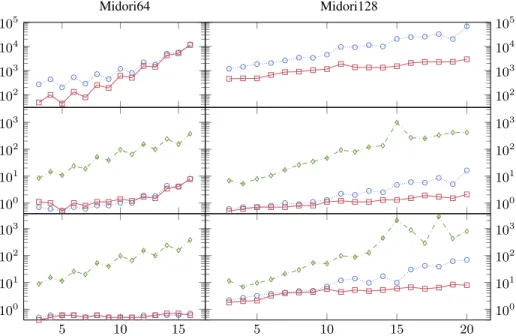
Results. On the top row of Fig. 4, we display the number of choice points needed to enumerate all Step1 solutions. GlobalGACexplores less choice points than GlobalFeas,
though the difference is very small for Midori64 when r ≥ 12.
In the middle row of Fig. 4, we display the CPU time spent to enumerate all Step1 solutions. For Midori64, the two Global variants have very similar times whereas, for Midori128, GlobalGACis faster than GlobalFeas. Advanced is much slower than Global.
In the bottom row of Fig. 4, we display the CPU time needed to solve the full MDC problem. For Midori64, GlobalFeas and GlobalGAChave very similar results, and are
much faster than Advanced. For Midori128, GlobalGACis faster than GlobalFeas, which
Midori64 Midori128 102 103 104 105 102 103 104 105 100 101 102 103 100 101 102 103 5 10 15 100 101 102 103 5 10 15 20 100 101 102 103
Fig. 4: Comparison of GlobalFeas( ), GlobalGAC( ), and Advanced ( ) for Midori.
The x-axis gives the number of rounds r, and the y-axis the number of choice points for Enum1
(up), and the run time for Enum1(Middle) and for Opt1+2(bottom). Times are in seconds.
5.2 Related-key MDC for AES
Description of the problem. Like Midori, AES iterates r rounds, and each round is composed of four operations. However, AES computes a new sub-key at each round according to a key schedule which combinesXORand SubBytes operations. Also, the MixColumns operation is different and it combines XORs with a finite field multipli-cation by constant coefficients. This multiplimultipli-cation is easily modelled at Step2 using table constraints. However, it cannot be modelled at Step1 and constraint (A3) is
re-placed with the following constraints which are derived from the MDS property of MixColumns(see [14] for more details):
∀i ∈ [0, r − 2], ∀k ∈ [0, 3], 3 X j=0 (∆Zi[k + 4j] + ∆Yi[k + 4j]) ∈ {0, 5, 6, 7, 8} ∀i1, i2∈ [0, r − 2], ∀k1, k2∈ [0, 3], 3 X j=0 (xi1i2k1k2j+ yi1i2k1k2j) ∈ {0, 5, 6, 7, 8}
where xi1i2k1k2jand yi1i2k1k2jare binary variables which are constrained as follows:
xi1i2k1k2j = 1 ⇔ δZi1[k1+ 4j] ⊕ δZi2[k2+ 4j] 6= 0
yi1i2k1k2j = 1 ⇔ δYi1[k1+ 4j] ⊕ δYi2[k2+ 4j] 6= 0
There exist three variants of AES, denoted AESl, where l ∈ {128, 192, 256} cor-responds to the number of bits in the key. The key schedule depends on l whereas all
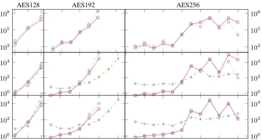
AES128 AES192 AES256 102 105 108 102 105 108 100 102 104 100 102 104 100 102 104 100 102 104
Fig. 5: Comparison of GlobalFeas( ), GlobalGAC( ), and Advanced ( ) for AES. The
x-axis gives the number of rounds r, and the y-axis the number of choice points for Enum1(up),
and the run time for Enum1(Middle) and Opt1+2(bottom). Times are in seconds.
other operations do not depend on l. For each key size l, we consider different values for the number of rounds r, ranging from 3 to an upper bound which depends on MDC probabilities: when increasing r, the probability decreases and it is useless to compute MDCs whenever the log2probability becomes smaller than −128.
Like in Section 5.1, we consider two problems: Enum1 aims at enumerating all
Step1 solutions, and Opt1+2aims at finding the optimal MDC.
Models for Enum1. We consider two CP models. Global is derived in a straightforward
way from the definition of AES and the MDS property by replacing allXORequations with an abstractXOR global constraint. It is implemented with Choco 4, and we con-sider two propagators (ensuring feasibility and GAC, respectively).
Advancedis the model introduced in [14] (which is more efficient than the ones of [15] and [20]). It uses a preprocessing step to infer new XORequations from the key schedule, and it adds new variables and constraints to remove Step2-inconsistent solutions by reasoning on equality relations between ∆jvariables. This model is much
more difficult to design than Global. It is implemented with Picat-SAT.
Models for Opt1+2. Like in Section 5.1, Global solves the two steps with a single
model implemented with Choco 4 whereas Advanced enumerates Step1 solutions with Picat-SAT and searches for optimal MDCs with Choco 4.
Results. On the top row of Fig. 5, we display the number of choice points needed to enumerate all Step1 solutions. In most cases, GlobalFeasexplores slightly more choice
points than GlobalGAC. However, for 5 instances of AES256, GlobalFeasexplores slightly
than ensuring feasibility) but not impossible as filtering has an impact on the variable ordering heuristic.
In the middle row of Fig. 5, we display the time spent to enumerate all Step1 so-lutions. In many cases, GlobalGACis faster than GlobalFeas, but the difference is often
rather small. Advanced is slower than Global when r ≤ 3 (resp. 6 and 8) for AES128 (resp. 192 and 256), but it has better scale-up properties and it becomes faster for larger values of r. In particular, Advanced is able to solve AES192 when r = 9 (resp. r = 10) in 1,326s (resp. 31,611s) whereas Global is not able to complete the run within a time limit of 200,000s.
In the bottom row of Fig. 5, we display the time needed to solve the full MDC problem. The performance of the three approaches are rather similar to the one in the middle row. However, for many instances the fact that the two steps are solved within a single model improves the solution process. This is the case, for example, for AES128 when r = 5. In this case, there are 103 Step1 solutions. If Advanced is more efficient than GlobalGACto enumerate these solutions (1,694s for Advanced instead of 2,656s
for GlobalGAC), Advanced needs much more time to find the optimal MDC (76,103s
instead of 6,096s).
5.3 Experimental results for the single-key problem
In the single-key differential attack, differences are introduced only in the initial text X0, and no difference is introduced in the key, i.e., δK = 0. Like for related-key, we
consider two problems: Enum1(to enumerate all Step1 solutions), and Opt1+2(to find
the optimal MDC). We also consider two block ciphers, i.e., Midori and AES. In all cases, we consider Global and Advanced models, and these models are obtained from related-key models by assigning 0 to all variables associated with the key.
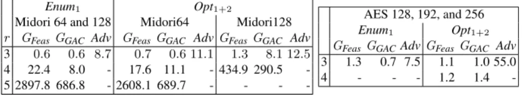
CPU times are reported in Table 1. For AES, the problem is the same whatever the length of the key (128, 192, or 256), as there is no difference in the key. For Midori, Enum1is the same whatever the length of the initial text (64 or 128) as bit sequences
are abstracted by Boolean values. However, Opt1+2 is different for Midori64 and
Mi-dori128. Surprisingly, single-key problems are much harder to solve than related-key ones, though the size of the search space is smaller (as all variables associated with the key are assigned to 0). This comes from the fact that the number of differences (defined by the constant n in Fig. 2) is strongly increased: n is increased from 3 (resp. 4 and 5) to 7 (resp. 16 and 23) when r = 3 (resp. 4 and 5) for Midori, and from 5 (resp. 12) to 9 (resp. 25) when r = 3 (resp. 4) for AES.
Results for Midori. Advancedfinds much more Step1 solutions than Global: it finds 64 (resp. 4,908) solutions when r = 3 (resp. 4), whereas Global finds 16 (resp. 68) solu-tions. Every solution found by Advanced and not by Global is Step2 inconsistent and Advancedspends a lot of time to enumerate these useless solutions. Hence, Advanced is not able to solve Midori within one hour when r > 3. When r = 4, Advanced is able to solve Enum1in 59,036s, but it is not able to solve Opt1+2within a reasonable amount
of time because most Step1 solutions are Step2 inconsistent.
Globalis able to solve up to r = 5 (resp. r = 4) for Midori64 (resp. Midori128). Step2 is much harder for Midori128 than for Midori64 because differential variables
Enum1 Opt1+2
Midori 64 and 128 Midori64 Midori128 r GFeasGGAC Adv GFeasGGAC AdvGFeasGGAC Adv
3 0.6 0.6 8.7 0.7 0.6 11.1 1.3 8.1 12.5 4 22.4 8.0 - 17.6 11.1 - 434.9 290.5 -5 2897.8 686.8 - 2608.1 689.7 - - -
-AES 128, 192, and 256 Enum1 Opt1+2
GFeasGGACAdvGFeasGGAC Adv 3 1.3 0.7 7.5 1.1 1.0 55.0 4 - - - 1.2 1.4
-Table 1: Single-Key results: Time (in seconds) needed by GlobalFeas(GFeas), GlobalGAC(GGAC),
and Advanced (Adv) for Midori (left) and AES (right). We report ‘-’ when time exceeds 3600s.
associated with the text take their values in [0, 255] for Midori128 and in [0, 16] for Midori64. Ensuring GAC often pays off and GlobalGACis faster than GlobalFeas, except
for Opt1+2/Midori128/r = 3.
Results for AES. When r = 3, both Enum1and Opt1+2are quickly solved, and Global
is an order faster than Advanced. When r = 4, there is a huge number of Step1 solutions (we have enumerated 1,715,652 solutions within a 24 hour time limit with GlobalGAC,
and all these solutions are Step2 consistent). Hence, Global fails at enumerating all Step1 solutions within a reasonable amount of time. However, when merging Step1 and Step2 models to solve Opt1+2, we find an optimal solution in less than 2s (the optimality
proof is trivial because all Pi[b] variables are assigned to the largest possible value).
When r = 4, the probability of the optimal MDC is equal to 2−150, which is smaller than 2−128. Hence, this MDC is useless to mount attacks. However, the fact that Global is able to enumerate a huge number of Step1 solutions in a reasonable amount of time opens new perspectives: we can search for a set of MDCs that share the same values in the initial text δX0and in the cipher text δXr, and combine these MDCs to find better
differentials.
6
Conclusion
We have introduced a new global constraint which eases the design of models for com-puting MDCs: these models are straightforwardly derived from problem definitions. This global constraint allows us to compute MDCs much faster than advanced models (which are much more difficult to design and which combine SAT and CP solvers) for single-key and related-key Midori, and for single-key AES. However, for related-key AES, it fails at solving the two largest instances of AES192 within a reasonable amount of time, and SAT has better scale-up properties for enumerating Step1 solutions. As pointed out in [14], clause learning is a key ingredient for solving this problem, and further work will aim at improving scale-up properties of Choco on this problem by adding clause learning to Choco.
We believe our new global constraint opens promising perspectives for cryptographs, and we aim at using it to solve new differential cryptanalysis problems such as those studied in [9] or [27], and new symmetric block ciphers such as Skinny [3].
Acknowledgement: This work has been funded by ANR DeCrypt (ANR-18-CE39-0007). We thank Charles Prud’homme for answering our numerous questions on Choco.
References
1. Abdelkhalek, A., Sasaki, Y., Todo, Y., Tolba, M., Youssef, A.: MILP modeling for (large) s-boxes to optimize probability of differential characteristics. IACR Trans. Symmetric Cryptol. 2017(4), 99–129 (2017)
2. Banik, S., Bogdanov, A., Isobe, T., Shibutani, K., Hiwatari, H., Akishita, T., Regazzoni, F.: Midori: A block cipher for low energy. In: ASIACRYPT. LNCS, vol. 9453, pp. 411–436. Springer (2015)
3. Beierle, C., Jean, J., K¨olbl, S., Leander, G., Moradi, A., Peyrin, T., Sasaki, Y., Sasdrich, P., Sim, S.M.: The SKINNY family of block ciphers and its low-latency variant MANTIS. In: CRYPTO 2016 - 36th Annual International Cryptology Conference,. Lecture Notes in Computer Science, vol. 9815, pp. 123–153. Springer (2016)
4. Biere, A.: Yet another local search solver and lingeling and friends entering the sat competi-tion 2014 pp. 39–40 (01 2014)
5. Biham, E.: New types of cryptoanalytic attacks using related keys (extended abstract). In: EUROCRYPT, LNCS 765. pp. 398–409. Springer (1993)
6. Biham, E., Shamir, A.: Differential cryptoanalysis of feal and n-hash. In: EUROCRYPT. LNCS, vol. 547, pp. 1–16. Springer (1991)
7. Biryukov, A., Nikolic, I.: Automatic search for related-key differential characteristics in byte-oriented block ciphers: Application to AES, camellia, khazad and others. In: Advances in Cryptology, LNCS 6110. pp. 322–344. Springer (2010)
8. Boussemart, F., Hemery, F., Lecoutre, C., Sais, L.: Boosting systematic search by weighting constraints. In: Proceedings of the 16th Eureopean Conference on Artificial Intelligence, ECAI’2004. pp. 146–150. IOS Press (2004)
9. Cid, C., Huang, T., Peyrin, T., Sasaki, Y., Song, L.: Boomerang connectivity table: A new cryptanalysis tool. In: EUROCRYPT. LNCS, vol. 10821, pp. 683–714. Springer (2018) 10. FIPS 197: Advanced Encryption Standard. Federal Information Processing Standards
Publi-cation 197 (2001), u.S. Department of Commerce/N.I.S.T.
11. Fouque, P., Jean, J., Peyrin, T.: Structural evaluation of AES and chosen-key distinguisher of 9-round AES-128. In: Advances in Cryptology - CRYPTO 2013 - Part I. LNCS, vol. 8042, pp. 183–203. Springer (2013)
12. G´erault, D.: Security Analysis of Contactless Communication Protocols. Ph.D. thesis, Uni-versit´e Clermont Auvergne (2018)
13. G´erault, D., Lafourcade, P.: Related-key cryptanalysis of midori. In: Progress in Cryptology - INDOCRYPT 2016. LNCS, vol. 10095, pp. 287–304 (2016)
14. Gerault, D., Lafourcade, P., Minier, M., Solnon, C.: Computing AES related-key differential characteristics with constraint programming. Artif. Intell. 278 (2020)
15. G´erault, D., Minier, M., Solnon, C.: Constraint programming models for chosen key differ-ential cryptanalysis. In: CP. LNCS, vol. 9892, pp. 584–601. Springer (2016)
16. Knudsen, L.: Truncated and higher order differentials. In: Fast Software Encryption. pp. 196–211. Springer (1995)
17. K¨olbl, S., Leander, G., Tiessen, T.: Observations on the SIMON block cipher family. In: CRYPTO - 35th Annual Cryptology Conference. LNCS, vol. 9215, pp. 161–185. Springer (2015)
18. Lafitte, F.: Cryptosat: a tool for sat-based cryptanalysis. IET Information Security 12(6), 463–474 (2018)
19. Le cl´ement de saint Marcq, V., Schaus, P., Solnon, C., Lecoutre, C.: Sparse-Sets for Domain Implementation. In: CP workshop on Techniques foR Implementing Constraint program-ming Systems (TRICS) (2013), https://hal.archives-ouvertes.fr/hal-01339250
20. Minier, M., Solnon, C., Reboul, J.: Solving a Symmetric Key Cryptographic Problem with Constraint Programming. In: Workshop on Constraint Modelling and Reformulation (Mod-Ref). pp. 1–13 (2014)
21. Mouha, N., Preneel, B.: A proof that the ARX cipher salsa20 is secure against differential cryptanalysis. IACR Cryptology ePrint Archive 2013, 328 (2013)
22. Prud’homme, C., Fages, J.G., Lorca, X.: Choco Documentation. TASC, INRIA Rennes, LINA CNRS UMR 6241, COSLING S.A.S. (2016), http://www.choco-solver.org
23. Soos, M., Nohl, K., Castelluccia, C.: Extending SAT solvers to cryptographic problems. In: SAT. LNCS, vol. 5584, pp. 244–257. Springer (2009)
24. Sun, L., Wang, W., Wang, M.: More accurate differential properties of led64 and midori64. IACR Transactions on Symmetric Cryptology 2018(3), 93–123 (2018)
25. Sun, S., G´erault, D., Lafourcade, P., Yang, Q., Todo, Y., Qiao, K., Hu, L.: Analysis of aes, skinny, and others with constraint programming. In: 24th International Conference on Fast Software Encryption (2017)
26. Sun, S., Hu, L., Wang, P., Qiao, K., Ma, X., Song, L.: Automatic security evaluation and (related-key) differential characteristic search: Application to simon, present, lblock, DES(L) and other bit-oriented block ciphers. In: ASIACRYPT. LNCS, vol. 8873, pp. 158–178. Springer (2014)
27. Todo, Y., Isobe, T., Hao, Y., Meier, W.: Cube attacks on non-blackbox polynomials based on division property. In: CRYPTO. LNCS, vol. 10403, pp. 250–279. Springer (2017)
28. Zhou, N.F., Kjellerstrand, H., Fruhman, J.: Constraint Solving and Planning with Picat. Springer (2015)