Convex nonnegative matrix factorization with missing data

(1)

HAL Id: hal-01346492

https://hal-amu.archives-ouvertes.fr/hal-01346492

Submitted on 7 Oct 2016

HAL is a multi-disciplinary open access

archive for the deposit and dissemination of

sci-entific research documents, whether they are

pub-lished or not. The documents may come from

teaching and research institutions in France or

abroad, or from public or private research centers.

L’archive ouverte pluridisciplinaire HAL, est

destinée au dépôt et à la diffusion de documents

scientifiques de niveau recherche, publiés ou non,

émanant des établissements d’enseignement et de

recherche français ou étrangers, des laboratoires

publics ou privés.

Convex nonnegative matrix factorization with missing

data

Ronan Hamon, Valentin Emiya, Cédric Févotte

To cite this version:

Ronan Hamon, Valentin Emiya, Cédric Févotte. Convex nonnegative matrix factorization with missing

data. IEEE International Workshop on Machine Learning for Signal Processing, Sep 2016, Vietri sul

Mare, Salerno, Italy. �hal-01346492�

(2)

2016 IEEE INTERNATIONAL WORKSHOP ON MACHINE LEARNING FOR SIGNAL PROCESSING, SEPT. 13–16, 2016, SALERNO, ITALY

CONVEX NONNEGATIVE MATRIX FACTORIZATION WITH MISSING DATA

Ronan Hamon, Valentin Emiya

˚

Aix Marseille Univ, CNRS, LIF, Marseille, France

C´edric F´evotte

CNRS & IRIT, Toulouse, France

ABSTRACT

Convex nonnegative matrix factorization (CNMF) is a variant of nonnegative matrix factorization (NMF) in which the com-ponents are a convex combination of atoms of a known dic-tionary. In this contribution, we propose to extend CNMF to the case where the data matrix and the dictionary have miss-ing entries. After a formulation of the problem in this context of missing data, we propose a majorization-minimization al-gorithm for the solving of the optimization problem incurred. Experimental results with synthetic data and audio spectro-grams highlight an improvement of the performance of re-construction with respect to standard NMF. The performance gap is particularly significant when the task of reconstruction becomes arduous, e.g. when the ratio of missing data is high, the noise is steep, or the complexity of data is high.

Index Terms— matrix factorization, nonnegativity, low-rankness, matrix completion, spectrogram inpainting

1. INTRODUCTION

Convex NMF (CNMF) [1] is a special case of nonnegative matrix factorization (NMF) [2], in which the matrix of com-ponents is constrained to be a linear combination of atoms of a known dictionary. The term “convex” refers to the con-straint of the linear combination, where the combination co-efficients forming each component are nonnegative and sum to 1. Compared to the fully unsupervised NMF setting, the use of known atoms is a source of supervision that may guide learning based on this additional data: in particular, an inter-esting case of CNMF consists in auto-encoding the data them-selves, by defining the atoms as the data matrix. CNMF has been of interest in a number of contexts, such as clustering, data analysis, face recognition, or music transcription [1, 3]. It is also related to the self-expressive dictionary-based repre-sentation proposed in [4].

An issue that has not yet been addressed is when the data matrix has missing coefficients. Such an extension of CNMF is worth being considered, as it opens the way to data-reconstruction settings with nonnegative low-rank con-straints, which covers several relevant applications. One

˚_{This work was supported by ANR JCJC program MAD (ANR-}

14-CE27-0002).

example concerns the field of image or audio inpainting [5, 6, 7, 8], where CNMF may improve the current reconstruction techniques. In inpainting of audio spectrograms for example, setting up the dictionary to be a comprehensive collection of notes from a specific instrument may guide the factorization toward a realistic and meaningful decomposition, increasing the quality of the reconstruction of the missing data. In this contribution, we also consider the case where the dictionary may have missing coefficients itself.

The paper is organized as follows. Section 2 formulates CNMF in the presence of missing entries in the data ma-trix and in the dictionary. Section 3 describes the proposed majorization-minimization (MM) algorithm. Sections 4 and 5 report experimental results with synthetic data and audio spectrograms.

2. CONVEX NONNEGATIVE MATRIX FACTORIZATION WITH MISSING DATA

2.1. Notations and definitions

For any integer N , the integer set t1, 2, . . . , N u is denoted by rN s. The coefficients of a matrix A P RM ˆN are denoted by either amn or rAs_mn. The element-wise matrix product,

matrix division and matrix power are denoted by A.B, A B

andA.γ_{, respectively where}_{A and B are matrices with same}

dimensions and γ is a scalar. 0 and 1 denote vectors or ma-trices composed of zeros and ones, respectively, with dimen-sions that can be deduced from the context. The element-wise negation of a binary matrixM is denoted by ¯M fi 1 ´ M.

2.2. NMF and Convex NMF

NMF consists in approximating a data matrixV P RF ˆN` as

the productWH of two nonnegative matrices W P RF ˆK`

andH P RKˆN

` . Often, K ă min pF, N q, such that WH

is a low-rank approximation ofV. Every sample vn, the

n-th column ofV, is thus decomposed as a linear combination of K elementary components or patternsw1, . . . ,wK P RF_`,

the columns ofW. The coefficients of the linear combination are given by the n-th columnhnofH.

In [9] and [10], algorithms have been proposed for the un-supervised estimation ofW and H from V, by minimization

(3)

of the cost function DβpV|WHq “

ř

f ndβpvf n|rWHsf nq,

where dβpx|yq is the β-divergence defined as:

dβpx|yq fi $ ’ ’ ’ ’ & ’ ’ ’ ’ % 1 βpβ´1q`x β ` pβ ´ 1q yβ´ βxyβ´1˘ for β P Rz t0, 1u x logx_y ´ x ` y for β “ 1 x y ´ log x y´ 1 for β “ 0 (1)

When ill-defined, we set by convention dβp0|0q “ 0.

CNMF is a variant of NMF in which W “ SL. S “ rs1, . . . ,sPs P RF ˆP` is a nonnegative matrix of atoms and

L “ rl1, . . . ,lKs P RP ˆK` is the so-called labeling matrix.

Each dictionary elementwk is thus equal toSlk, with

usu-ally P ąą K, and the data is in the end decomposed as V “ SLH. The scale indeterminacy between L and H may be lifted by imposing }lk}1 “ 1, in which case wk is

pre-cisely a convex combination of the elements of the subspace S. CNMF can be related to the so-called archetypal analysis [11], but without considering any nonnegativity constraint.

The use of known examples in S can then be seen as a source of supervision that guides learning. A special case of CNMF is obtained by setting S “ V, thus auto-encoding the data asVLH. This particular case is studied in depth in [1]. In this paper, we consider the general case forS, with or without missing data.

2.3. Convex NMF with missing data

We assume that some coefficients inV and S may be missing. Let_{V Ă rF s ˆ rNs be a set of pairs of indices that locates} the observed coefficients inV: pf, nq PV iff vf n is known.

Similarly, let_{S Ă rF s ˆ rP s be a set of pairs of indices that} locates the observed coefficients inS. The use of setsV and S may be reformulated equivalently by defining masking ma-tricesMV P t0, 1uF ˆN andMS P t0, 1uF ˆP fromV and S

as rMVsf nfi # 1 if pf, nq P_V 0 otherwise @pf, nq P rF s ˆ rN s (2) rMSsf pfi # 1 if pf, pq P_S 0 otherwise @pf, pq P rF s ˆ rP s (3)

A major goal in this paper is to estimate L, H and the missing entries inS, given the partially observed data matrix V. Denoting by So_{the set of observed/known dictionary}

ma-trix coefficients, our aim is to minimize the objective function

C pS, L, Hq fi DβpMV.V|MV.SLHq (4) subject to S P RF ˆP` , L P R P ˆK ` , H P R KˆN ` , and

MS.S “ MS.So. The particular case where the

dic-tionary equals the data matrix itself is obtained by setting pMS,Soq fi pMV,Vq.

Algorithm 1 CNMF with missing data Require: V, So_,_M

V,MS , β

InitializeS, L, H with random nonnegative values loop UpdateS: S Ð MS.So` (5) M_S.S. ¨ ˝ ´ M_V. pSLHq.pβ´2q.V ¯ pLHqT ´ M_V. pSLHq.pβ´1q ¯ pLHqT ˛ ‚ .γpβq UpdateL: L Ð L. ¨ ˝ ST´_M V. pSLHq.pβ´2q.V ¯ HT ST´_M V. pSLHq.pβ´1q ¯ HT ˛ ‚ .γpβq (6) UpdateH: H Ð H. ¨ ˝ pSLqT ´ MV. pSLHq.pβ´2q.V ¯ pSLqT ´ MV. pSLHq.pβ´1q ¯ ˛ ‚ .γpβq (7) RescaleL and H: @k P rKs , hkÐ }lk}1ˆ hk (8) lkÐ lk }lk}1 (9) end loop return S, L, H 3. PROPOSED ALGORITHM

3.1. General description of the algorithm

Algorithm 1 extends the algorithm proposed in [9] for com-plete CNMF with the β-divergence to the case of missing en-tries inV or S. The algorithm is a block-coordinate descent procedure in which each block is one the three matrix factors. The updates of each block/factor is obtained via majorization-minimization (MM), a classic procedure that consists in itera-tively minimizing a tight upper bound (called auxiliary func-tion) of the objective function. In the present setting, the MM procedure leads to multiplicative updates, characteristic of many NMF algorithms, that automatically preserve non-negativity given positive initialization.

3.2. Detailed updates

We consider the optimization of C pS, L, Hq with respect to each of its three arguments individually, using MM. Current updates are denoted with a tilde, i.e., rS, rL and rH. We start by recalling the definition of an auxiliary function:

Definition 1 (Auxiliary function). The mapping G ´

(4)

RIˆJ` ˆ R IˆJ

` ÞÑ R`is an auxiliary function to C pAq iff

#

@A P RIˆJ` , C pAq “ G pA|Aq

@A, rA P RIˆJ` , C pAq ď G

´

A| rA¯. (10)

The iterative minimization of G pA|Aq with respect to A, with replacement of rA at every iteration, monotonically de-creases the objective C pAq until convergence. As explained in detail in [9], the β-divergence may be decomposed into the sum of a convex term qdβp.|.q, a concave term udβp.|.q and a

constant term cst. The first two terms can be majorized using routine Jensen and tangent inequalities, respectively, leading to tractable updates. The auxiliary functions used to derive Algorithm 1 are given by the three following propositions1 and the monotonicity of the algorithm follows by construc-tion.

Proposition 1 (Auxiliary function forS).

Let rS P RF ˆP` be such that @pf, nq P rF s ˆ rN s, ˜vf n ą 0,

and @pf, pq P rF s ˆ rP s, ˜sf p ą 0, where rV fi rSLH. Then

is an auxiliary function toC pS, L, Hq with respect to S and its minimum is given by equation(5). The auxiliary function decouples with respect to the individual coefficients ofS and as such, the constraintMS.S “ MS.Sois directly imposed

by only updating the coefficients ofS with indices in ¯S. Proposition 2 (Auxiliary function forL).

Let rL P RP ˆK` be such that @pf, nq P rF s ˆ rN s, ˜vf n ą 0

and @pp, kq P rP s ˆ rKs, ˜lpk ą 0, where rV fi SrLH. Then

1_{The proof of these propositions are available in the extended version at}

https://hal-amu.archives-ouvertes.fr/hal-01346492.

is an auxiliary function to C pS, L, Hq with respect to L and its minimum subject to MS.S “ MS.So for MS P

t0, 1uF ˆP andSo

P RF ˆP` is given by equation(6).

Proposition 3 (Auxiliary function forH). Let us defineW fi SL and let rH P RKˆN

` be such that

@pf, nq P rF s ˆ rN s,rvf n ą 0 and @pk, nq P rKs ˆ rN s, rhkną 0, where rV fi W rH. Then the function

is an auxiliary function toC pS, L, Hq with respect to H and its minimum is given by equation(7).

4. EXPERIMENT ON SYNTHETIC DATA

4.1. Experimental setting

The objective of this experiment is to analyze the performance of CNMF for reconstructing missing data, by comparing it with the regular NMF. We consider a data matrixV˚_{of rank}

K˚ _{synthesized under the CNMF model} _V˚ _{“ S}˚_L˚_H˚_,

where the matrix of atomsS˚ _{and the ground truth factors}

L˚_and_H˚_{are generated as the absolute values of Gaussian}

noise. It is worth noting that V˚ _{is also consistent with a}

NMF model by definingW˚_{“ S}˚_L˚_{. A perturbed data}

ma-trixV is obtained by considering a multiplicative noise, ob-tained using a Gamma distribution with mean 1 and variance

1

α. Hence the parameter α controls the importance of the

per-turbation. The maskMVof known elements inV is derived

by considering missing coefficients randomly and uniformly distributed over the matrix, such that the ratio of missing val-ues is equal to σV. Generation of data is repeated 3 times, as

well as the generation of the masks. Results are averaged over these repetitions.

From a matrixV with missing entries, NMF and CNMF with missing values are applied using K components. Only the case where β “ 2 has been considered in this experiment. In both algorithms, the convergence is reached when the rel-ative difference of the cost function between two iterations is below 10´5_{. 3 repetitions are performed using different}

random initialization, and the best instance (i.e., the instance which minimizes the cost function) is retained. The recon-structed data matrix is obtained as rV “ SLH.

The reconstruction error is obtained by computing the β-divergence between the noiseless data matrixV˚_{, and the}

(5)

along the missing coefficients only, as etest“ 1 ř ijr ¯MVsij dβp ¯MV.V˚, ¯MVVqr (11)

where ¯MVis the mask of unknown elements inV. In the case

of CNMF, we consider two choices forS: the data matrix V with missing values, and the ground truth matrix of atomsS˚_,

considered here without missing values.

The following parameters are fixed: F “ 100, N “ 250, P “ 50, K˚_{“ 10, β “ 2. We particularly investigate the}

in-fluence of four factors: the number of estimated components K P r2, 14s; the ratio of missing data σV P r0.1, 0.9s in V,

i.e., of zeros inMV; the choice of the matrixS P tS˚,Vu for

the CNMF; the noise level α P r10, 5000s in V (α is inversely proportional to the variance of the noise).

4.2. Results

We first focus on the influence of the number of estimated components k for the case where the true dictionary is fully known. Figure 1 displays the test error with respect to the number of estimated components K, for two levels of noise. Performance of reconstruction obtained by NMF and CNMF withS “ S˚_{are plotted, for different values of ratio of}

miss-ing values in_V. 2 4 6 8 10 12 14 Number of components 10−2 10−1 100 Test error α = 100 2 4 6 8 10 12 14 Number of components 10−3 10−2 10−1 100 Test error α = 3000 σV= 0.2- NMF σV= 0.2- CNMF σV= 0.6- NMF σV= 0.6- CNMF σV= 0.8- NMF σV= 0.8- CNMF

Fig. 1. Test error vs. number of components. Two levels of noise are displayed: high noise level (α “ 100, left) and low noise level (α “ 3000, right).

These results show that the noise level has a high influence on the best number of estimated components. As expected, a high noise requires a strong regularization, obtained here by selecting a low value of K. On the contrary, when the noise is low, the best choice of K is closer to the true value K˚ _{“ 10. Similarly, when the number of missing data is}

low (σV “ 0.2), one should set K to K˚ “ 10, either for

CNMF or for NMF. When it gets higher, the optimal K gets lower in order to limit the effect of overfitting. In this case, the best number of components drops down to K “ 2, either

for CNMF or NMF, the former still performing better than the latter. These first results outline the difference between NMF and CNMF, emphasized in the next figures.

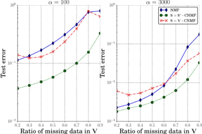
This comparison is augmented by considering the case whereS “ V, with respect to the ratio σV of missing values

inV. Figure 2 displays the performance of NMF and CNMF as a function of σV, for two noise levels. CNMF with the true

atoms (S “ S˚_{) gives the best results on the full range}

miss-ing data ratio. When there are very few missmiss-ing data and a low noise, NMF performs almost as well as CNMF. However, the NMF error increases much faster than the CNMF error as the number of missing data grows, or as the noise in data be-comes important. This higher sensitivity of NMF to missing data may be explained by overfitting since the number of free parameters in NMF is higher than in CNMF. In the case of CNMF withS “ V, the model cannot fit the data as well as CNMF withS “ S˚_{or as NMF. Consequently, the resulting}

modeling error is observed when there is few missing data, and when comparingS “ V and S “ S˚_{on all values.}

How-ever, it performs better than NMF at high values of σVsince

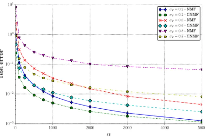
the constraintS “ V can be seen as a regularization. We finally investigate the robustness of methods by look-ing at the influence of the multiplicative noise, controlled by the parameter α, on the performance. Figure 3 shows the test error for the NMF and the CNMF withS “ S˚_{with respect}

to α and for some values of σV. As expected, the test

er-ror decreases according to the variance of the noise, inversely proportional to α. If a low value of α disrupts abruptly the performance of reconstruction (α ă 103_{), the test error is}

slightly decreasing for α ą 103_{. When the variance of the}

noise is close to zero (α “ 5000), the performance of NMF and CNMF are almost the same. The performance of recon-struction differs when the variance of the noise increases, as well as the ratio of missing values inV.

0.2 0.3 0.4 0.5 0.6 0.7 0.8 0.9

Ratio of missing data in V

10−2 10−1 100 Test error α = 100 0.2 0.3 0.4 0.5 0.6 0.7 0.8 0.9

10−3 10−2 10−1 100 Test error α = 3000 NMF S = S∗_{- CNMF} S = V- CNMF

Fig. 2. Test error vs. ratio of missing data inV, with K “ K˚_{. Two levels of noise are displayed: high noise level (α “}

(6)

0 1000 2000 3000 4000 5000 α 10−3 10−2 10−1 100 101 Test error σV= 0.2- NMF σV= 0.2- CNMF σV= 0.6- NMF σV= 0.6- CNMF σV= 0.8- NMF σV= 0.8- CNMF

Fig. 3. Test error vs. noise level α. Each curve describes the performance of reconstruction of missing data inV, with K “ K˚_{, according to the method and the ratio of missing}

data σV.

5. APPLICATION TO SPECTROGRAM INPAINTING

In order to illustrate the performance of the proposed algo-rithm on real data, we consider spectrograms of piano music signals, which are known to be well modeled by NMF meth-ods [12]. Indeed, NMF may provide a note-level decomposi-tion of a full music piece, each NMF component being the es-timated spectrum and activation of a single note. This approx-imation has proved successful and is also limited in terms of modelling error and of lack of supervision to guide the NMF algorithm. In such condition, we have designed an experi-ment with missing data to compare regular NMF against two CNMF variants: in the first one, we setS “ V; in the second one,S contains examples of all possible isolated note spectra from another piano.

5.1. Experimental setting

We consider 17 piano pieces from the MAPS dataset [13]. For each recording, the magnitude spectrogram is computed using a 46-ms sine window with 50%-overlap and 4096 frequency bins, the sampling frequency being 44.1kHz. MatrixV is created from the resulting spectrogram by selecting the F “ 500 lower-frequency part and the first five seconds, i.e., the N “ 214 first time frames. Missing data in V are artificially created by removing coefficients uniformly at random.

Three systems are compared, based on the test error de-fined as the β-divergence computed on the estimation of miss-ing data. In all of them, the number of component K is set to the true number of notes available from the dataset annotation and we set β “ 1. The first system is the regular NMF, ran-domly initialized. The second system is the proposed CNMF with pMS,Soq fi pMV,Vq. The third system is the proposed

CNMF withS “ D set as a specific matrix D of P “ 61 atoms. Each atom is a single-note spectrum extracted from

the recording of another piano instrument from the MAPS dataset, from C3 to C82.

5.2. Results

Figure 4 displays the test error with respect to the ratio of missing data in V, averaged over the 17 piano pieces. It clearly shows that the CNMF with the specific dictionaryS “ D is much more robust to missing data than the other two sys-tems. When less than 40% of data are missing, NMF performs slightly better; however, the NMF test error dramatically in-creases when more data are missing, by a factor 5.103when more than 80% data are missing. This must be due to overfit-ting since NMF has a large number of free parameters to be estimated from very few observations when data are missing. The performance of the CNMF system withS “ V probably suffers from modelling error when very few data are missing – since the columns ofV may not be able to combine into K components in a convex way. In the range 50 ´ 70%, its performance is similar to that of NMF. Beyond this range, it seems to be less prone to overfitting than NMF, probably due to less free parameters or to a regularization effect provided byS “ V.

0.2 0.3 0.4 0.5 0.6 0.7 0.8 0.9 1.0

10−3 10−2 10−1 100 101 102 Test error NMF ConvexNMF - S=D ConvexNMF - S=V

Fig. 4. Test error vs. missing data ratio in audio spectrograms.

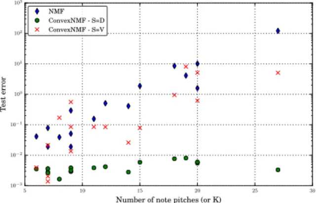
We now investigate the influence of the “complexity” of the audio signal on the test error when the ratio of missing data is set to the high value 80%. Figure 5 displays, for each music recording, the test error with respect to the number of different pitches for all notes in the piano piece, which also equals the number of component K used by each system. CNMF with S “ D performs better than NMF whatever the number of notes and the error increases by a small fac-tor along the represented range. NMF performs about five times worse for “easy” pieces, i.e., pieces composed of notes with about 6 different pitches and it performs about 104_times

worse when the number of pitches is larger than 25. CNMF

2_{The code of the experiments is available on the webpage of the MAD} project http://mad.lif.univ-mrs.fr/.

(7)

withS “ V performs slightly better than NMF. Since the number of components K increases equals the number of note pitches, those results confirm that NMF may highly suf-fer from overtraining while CNMF may not, being robust to missing data even for large values of K.

5 10 15 20 25 30

Number of note pitches (or K)

10−3 10−2 10−1 100 101 102 103 Test error NMF ConvexNMF - S=D ConvexNMF - S=V

Fig. 5. Test error vs. number of different note pitches for 80% missing data (each dot represents one piece of music).

6. CONCLUSION

In this paper, we have proposed an extension of convex non-negative matrix factorization in the case where missing data, as it has been previously presented for regular NMF. The pro-posed method can deal with missing values both in the data matrixV and in the dictionary S, which is particularly use-ful in the case S “ V where the data is autoencoded. In this framework, an algorithm has been provided and analyzed using a Majorization-Minimization (MM) scheme to guaran-tee the convergence to a local minimum. A large set of ex-periments on synthetic data showed promising results for this variant of NMF for the task of reconstruction of missing data, and validated the value of this approach. In many situations, CNMF outperforms NMF, especially when the ratio of miss-ing values is high and when the matrix dataV is noisy. This trend has been confirmed on real audio spectrograms of piano music. In particular, we have shown how the use of a generic set of isolated piano notes as atoms could dramatically en-hance the robustness to missing data.

This preliminary study indicates that it is worthy of fur-ther investigation, beyond the proposed settings where miss-ing values are uniformly distributed over the matrix. Further-more, the influence of missing values in the dictionary has not been completely assessed, as only the case whereS “ V has been taken into account. On the application side, this ap-proach could give new insight in many problems dealing with estimation of missing data.

7. REFERENCES

[1] C. Ding, Tao Li, and M.I. Jordan, “Convex and semi-nonnegative matrix factorizations,” IEEE Trans. Pattern Anal. Mach. Intell., vol. 32, no. 1, pp. 45–55, Jan. 2010. [2] D.D. Lee and H.S. Seung, “Learning the parts of objects by non-negative matrix factorization,” Nature, vol. 401, no. 6755, pp. 788–791, 1999.

[3] E. Vincent, N. Bertin, and R. Badeau, “Adaptive har-monic spectral decomposition for multiple pitch estima-tion,” IEEE Trans. Audio, Speech, Language Process., vol. 18, no. 3, pp. 528–537, Mar. 2010.

[4] E. Elhamifar and R. Vidal, “Sparse subspace clustering: Algorithm, theory, and applications,” IEEE Trans. Pat-tern Anal. Mach. Intell., vol. 35, no. 11, pp. 2765–2781, 2013.

[5] M. Bertalmio, G. Sapiro, V. Caselles, and C. Ballester, “Image inpainting,” in Proc of SIGGRAPH. ACM, 2000, pp. 417–424.

[6] P. Smaragdis, B. Raj, and M. Shashanka, “Missing data imputation for spectral audio signals,” in Proc. of MLSP, Grenoble, France, Sept. 2009.

[7] J. Le Roux, H. Kameoka, N. Ono, A. De Cheveigne, and S. Sagayama, “Computational auditory induction as a missing-data model-fitting problem with bregman divergence,” Speech Communication, vol. 53, no. 5, pp. 658–676, 2011.

[8] D.L. Sun and R. Mazumder, “Non-negative matrix com-pletion for bandwidth extension: A convex optimization approach,” in Proc. of MLSP, Sept. 2013, pp. 1–6. [9] C. F´evotte and J. Idier, “Algorithms for nonnegative

ma-trix factorization with the β-divergence,” Neural Com-put., vol. 23, no. 9, pp. 2421–2456, 2011.

[10] M. Nakano, H. Kameoka, J. Le Roux, Y. Kitano, N. Ono, and S. Sagayama, “Convergence-guaranteed multiplicative algorithms for nonnegative matrix factor-ization with β-divergence,” Proc. of MLSP, vol. 10, pp. 1, 2010.

[11] A. Cutler and L. Breiman, “Archetypal analysis,” Tech-nometrics, vol. 36, no. 4, pp. 338–347, 1994.

[12] C. F´evotte, N. Bertin, and J-L Durrieu, “Nonnegative matrix factorization with the Itakura-Saito divergence: With application to music analysis,” Neural Comput., vol. 21, no. 3, pp. 793–830, 2009.

[13] V. Emiya, R. Badeau, and B. David, “Multipitch esti-mation of piano sounds using a new probabilistic spec-tral smoothness principle,” IEEE Trans. Audio, Speech, Language Process., vol. 18, no. 6, pp. 1643–1654, 2010.

(8)

A. PROOFS

We detail the proofs of Propositions 1 and 2. The proof of Proposition 3 is straithforward using the same methodology. We first recall preliminary elementss from [9]. The β-divergence dβpx|yq can be decomposed as a sum of a convex term, a

concave term and a constant term with respect to its second variable y as

dβpx|yq “ qdβpx|yq ` udβpx|yq ` dβpxq (12)

This decomposition is not unique. We will use decomposition given in [9, Table 1], for which we have the following derivatives w.r.t. variable y: q d1 βpx|yq fi $ ’ & ’ % ´xyβ´2 if β ă 1 yβ´2_{py ´ xq} _{if 1 ď β ď 2} yβ´1 _{if β ą 2} (13) u d1 βpx|yq fi $ ’ & ’ % yβ´1 _{if β ă 1} 0 if 1 ď β ď 2 ´xyβ´2 if β ą 2 (14)

A.1. Update ofS (Proof of Proposition 1)

We prove Proposition 1 by first constructing the auxiliary function (Proposition 4 below) and then focussing on its minimum (Proposition 5 below). Due to separability, the update ofS P RF ˆP` relies on the update of each of its columns. Hence, we only

derive the update for a vectors P RP `.

Definition 2 (Objective function CSpsq). For v P RN`,L P R P ˆK ` ,H P R KˆN ` ,m P t0, 1u N ,mo P t0, 1uP,s P RP `, let us define CSpsq fi ÿ n mn ” q Cnpsq ` uCnpsq ı ` C (15) 0where q Cnpsq fi qdβ`vn|“sTLH ‰ n˘ ,Cunpsq fi udβ`vn|“s T_LH‰ n ˘ and C fi dβpm.vq ` λdβpmo.soq (16)

Proposition 4 (Auxiliary function GSps|rsq for CSpsq). Letrs P R

P

` be such that @n,rvn ą 0 and @p,rsp ą 0, wherev fir “sT_LH‰T

. Then the functionGSps|rsq defined by

is an auxiliary function forCSpsq.

Proof. We trivially have GSps|sq “ CSpsq. We use the separability in n and in p in order to upper bound each convex term

q

Cnpsq and each concave term uCnpsq.

Convex term qCnpsq. Let us prove that qGnps|rsq ě qCnpsq. LetP be the set of indices such that rLHspn‰ 0 and define, for

p P_P, r λpnfi rLHs_pnrsp r vn “ rLHspnr sp ř p1_PPrLHsp1nrsp1 . (19)

(9)

We haveř_pPPrλpn“ 1 and q Gnps|rsq “ ÿ pPP r λpndqβ ˜ vn| rLHs_pnsp r λpn ¸ ě qdβ ˜ vn| ÿ pPP r λpn rLHs_pnsp r λpn ¸ “ qdβ ˜ vn| P ÿ p“1 rLHs_pnsp ¸ “ qCnpsq (20)

Concave term uCnpsq. We have uGnps|rsq ě uCnpsq since uCnpsq is concave and s ÞÑ uGnps|rsq is a tangent plane to uCnpsq inrs:

u Gnps|rsq “ udβpvn|rvnq ` ÿ p u d1 β ˜ vn| ÿ p1 rLHs_p1nrsp1 ¸ rLHs_pnpsp´rspq “ uCnprsq `∇ uCnprsq , s ´rs (21)

Proposition 5 (Minimum of GSps|rsq). The minimum of s ÞÑ GSps|rsq subject to the constraint m

o_{.s “ m}o_.so_{is reached at} sMM_with @p, sMMp fi $ ’ & ’ % r sp ˆř nmnvr β´2 n vnrLHspn ř nmnrv β´1 n rLHspn ˙γpβq ifmo_p“ 0 so p ifmop“ 1. (22)

Proof. Since variable spis fixed for p such that mop “ 1, we only consider variables sp for p such that mop “ 0. The related

penalty term in GSps|rsq vanishes when m

o

p“ 0. Using (13) and (14), the minimum is obtained by cancelling the gradient

∇spGSps|rsq “ ÿ n mnLHpn „ q d1 β ˆ vn|rvn sp r sp ˙ ` ud1 βpvn|rvnq  (23)

and by considering that the Hessian matrix is diagonal with nonnegative entries since qdβpx|yq is convex:

∇2 spGSps|rsq “ ÿ n mnrvn LHpn r sp q d2 β ˆ vn|rvn sp r sp ˙ ě 0. (24)

A.2. Update ofL (Proof of Proposition 2)

We proove Proposition 2 by first constructing the auxiliary function (Proposition 6 below) and then focussing on its minimum (Proposition 7 below). As opposed to the update ofS, no separability is considered here.

Definition 3 (Objective function CLplq). For v P RF`,S P R F ˆP ` ,H P R KˆN ` ,M P t0, 1u F ˆN_, L P RP ˆK` , let us define CLpLq fi ÿ f n mf n ” q Cf npLq ` uCf npLq ı ` C (25) where q Cf npLq fi qdβ ´ vf n| rSLHsf n ¯ , uCf npLq fi udβ ´ vf n| rSLHsf n ¯ and C fi dβpM.Vq . (26)

Proposition 6 (Auxiliary function GL

´

L|rL¯for CLpLq). Let rL P RP ˆK` be such that @f, n, rVf n ą 0 and @p, k, rLpk ą 0,

where rV fi SrLH. Then the function GL

´ L|rL¯defined by GL ´ L|rL¯fiÿ f n mf n ” q Gf n ´ L|rL¯` uGf n ´ L|rL¯ı` C (27)

(10)

is an auxiliary function forCLpLq.

Proof. We trivially have GLpL|Lq “ CLpLq. In order to prove that GL

´

L|rL¯ě CLpLq, we use the separability in f and n

and we upper bound the convex terms qCf npLq and the concave terms uCf npLq.

Convex term qCf npLq. Let us prove that qGf n

´

L|rL¯ě qCf npLq. LetP be the set of indices such that sf p‰ 0,K be the set of

indices such that hkn‰ 0 and define, for pp, kq PP ˆ K,

r λf pknfi sf prlpkhkn r vf n “_ř sf prlpkhkn pp1_,k1_qPPˆKsf p1rlp1k1hk1n . (30) We haveř_pp,kqPPˆKλrf pkn“ 1 and q Gf n ´ L|rL¯“ ÿ pp,kqPPˆK r λf pkndq_β ˜ vf n| sf plpkhkn r λf pkn ¸ (31) ě qdβ ¨ ˝vf n| ÿ pp,kqPPˆK r λf pkn sf plpkhkn r λf pkn ˛ ‚“ qdβ ˜ vf n| P ÿ p“1 K ÿ k“1 sf plpkhkn ¸ “ qCf npLq (32)

Concave term uCf npLq. We have uGf n

´

L|rL¯ě uCf npLq since uCf npLq is concave and L ÞÑ uGf n

´ L|rL¯is a tangent plane to u Cf npLq in rL: u Gf n ´ L|rL¯“ udβpvf n|rvf nq ` ÿ pk u d1β ˜ vf n| ÿ p1_k1 sf p1rlp1_k1h_k1_n ¸ sf phkn ´ lpk´ rlpk ¯ (33) “ uCf n ´ r L¯` D ∇ uCf n ´ r L¯,L ´ rLE (34) Proposition 7 (Minimum of GL ´ L|rL¯). The minimum ofL ÞÑ GL ´ L|rL¯is reached atLMM_with @p, k, lp,kMMfi $ ’ & ’ % lp,k ˆř f nsf pmf nvr β´2 f n vf nhkn ř f nsf pmf nvr β´1 f n hkn ˙γpβq ifM ‰ 0 lp,kotherwise. (35)

Proof. Using (13) and (14), the minimum is obtained by cancelling the gradient

∇lpkGL ´ L|rL¯“ÿ f n mf nsf phkn « q d1 β ˜ vf n|vrf n lpk rlpk ¸ ` ud1 βpvf n|rvf nq ff (36)

and by considering that the Hessian matrix is diagonal with nonnegative entries since qdβpx|yq is convex:

∇2 lpkGL ´ L|rL¯“ÿ f n mf nrvf n sf phkn r lpk q d2 β ˜ vf n|rvf n lpk r hpk ¸ ě 0. (37)