Composition structures for system representation

(1)

Composition Structures for System Representation

by

Guolong Su

B.Eng. Electronic Eng., Tsinghua University, China (2011)

S.M. EECS, Massachusetts Institute of Technology (2013)

Submitted to the Department of Electrical Engineering and Computer

Science

in partial fulﬁllment of the requirements for the degree of

Doctor of Philosophy in Electrical Engineering and Computer Science

at the

MASSACHUSETTS INSTITUTE OF TECHNOLOGY

June 2017

c

⃝ Massachusetts Institute of Technology 2017. All rights reserved.

Author . . . .

Department of Electrical Engineering and Computer Science

May 19, 2017

Certiﬁed by . . . .

Alan V. Oppenheim

Ford Professor of Engineering

Thesis Supervisor

Accepted by . . . .

Leslie A. Kolodziejski

Professor of Electrical Engineering and Computer Science

Chair, Department Committee on Graduate Theses

(2)

(3)

Composition Structures for System Representation

by

Guolong Su

Submitted to the Department of Electrical Engineering and Computer Science on May 19, 2017, in partial fulﬁllment of the

requirements for the degree of

Doctor of Philosophy in Electrical Engineering and Computer Science

Abstract

This thesis discusses parameter estimation algorithms for a number of structures for system representation that can be interpreted as different types of composition. We refer to the term composition as the systematic replacement of elements in an object by other object modules, where the objects can be functions that have a single or multiple input variables as well as operators that work on a set of signals of interest. In general, composition structures can be regarded as an important class of constrained parametric representations, which are widely used in signal processing. Different types of composition are considered in this thesis, including multivariate function composition, operator composition that naturally corresponds to cascade systems, and modular composition that we refer to as the replacement of each delay element in a system block diagram with an identical copy of another system module. There are a number of potential advantages of the use of composition structures in signal processing, such as reduction of the total number of independent parameters that achieves representational and computational efficiency, modular structures that benefit hardware implementation, and the ability to form more sophisticated models that can represent significantly larger classes of systems or functions.

The first part of this thesis considers operator composition, which is an alternative interpretation of the class of cascade systems that has been widely studied in signal processing. As an important class of linear time-invariant (LTI) systems, we develop new algorithms to approximate a two-dimensional (2D) finite impulse response (FIR) filter as a cascade of a pair of 2D FIR filters with lower orders, which can gain computational efficiency. For nonlinear systems with a cascade structure, we generalize a two-step parameter estimation algorithm for the Hammerstein model, and propose a generalized all-pole modeling technique with the cascade of multiple nonlinear memoryless functions and LTI subsystems.

The second part of this thesis discusses modular composition, which replaces each delay element in a FIR filter with another subsystem. As an example, we propose the modular Volterra system where the subsystem has the form of the Volterra series. Given statistical information between input and output signals, an algorithm is proposed to estimate the coefficients of the FIR filter and the kernels of the Volterra

(4)

subsystem, under the assumption that the coeﬃcients of the nonlinear kernels have suﬃciently small magnitude.

The third part of this thesis focuses on composition of multivariate functions. In particular, we consider two-level Boolean functions in the conjunctive or disjunctive normal forms, which can be considered as the composition of one-level multivariate Boolean functions that take the logical conjunction (or disjunction) over a subset of binary input variables. We propose new optimization-based approaches for learning a two-level Boolean function from a training dataset for classiﬁcation purposes, with the joint criteria of accuracy and simplicity of the learned function.

Thesis Supervisor: Alan V. Oppenheim Title: Ford Professor of Engineering

(5)

Acknowledgments

I would like to sincerely express my gratitude to my supervisor Prof. Alan V. Oppenheim for his wonderful guidance, sharp insights, unconventional creativity, and strong mastery of the big picture. It has been my great privilege to work with Al, who truly cares about the comprehensive development and the best interests of his students. Among Al’s various contributions to the development of this thesis, I would like to especially thank Al for his intentionally cultivating my independence and overall maturity, while carefully and subtly providing a safety net. I benefited significantly from Al’s research style of free association, which tries to connect seemingly unrelated topics but can finally lead to unexpected inspiration. Moreover, I appreciate Al encouraging me to step back from the technical aspects and distill a deeper conceptual understanding for the work that I have done. Having attended Al’s lectures for the course Discrete-time Signal Processing in multiple semesters as a student and as a teaching assistant, I am impressed and motivated by Al’s enthusiasm and devotion to teaching, for which (and for other things) he always aims for excellence and takes the best efforts to further improve, even on the materials that he is so familiar with. Al, thank you for teaching me the way to be a good teacher. In addition, I am very grateful for Al’s various warm and voluntary help on non-academic issues.

I am fully grateful to the other members of my thesis committee, Prof. George C. Verghese and Dr. Sefa Demirtas, for their involvement in the development of my research project and their great suggestions in both the committee and individual meetings, which had significant contributions especially in clarifying the concepts and shaping this thesis. Aside from this thesis, I would like to thank Al and George for offering me the opportunity to work on the exercises of their new book Signals, Systems and Inference, which became a good motivation for me to gain deeper knowledge about related topics such as Wiener filtering. Sefa, I am so fortunate to have the great and enjoyable collaboration with you on polynomial decomposition algorithms when I was working towards my master’s degree, from which some ideas in

(6)

this thesis were inspired years later in an unexpected way; beyond our collaboration, you are a kind and supportive mentor, a frank and fun oﬃce mate, and a very responsible thesis reader, and I want to sincerely thank you for all of these.

I would like to have my sincere appreciation to Prof. Gregory W. Wornell and Prof. Stefanie S. Jegelka, who kindly granted me with another teaching assistantship opportunity for their course Inference and Information in Spring 2015, which turned out an excellent and precious experience for me. In addition to Greg’s passion and erudition, I really appreciate his amazing ability in distilling the essence from a complicated concept and illustrating it in a natural and enjoyable way that is easy to grasp. Greg and Stefanie, thank you for showing and training me on how to teach eﬀectively and for deepening my own understanding of the course materials that I feel attractive.

It is my great privilege to be a member of the “academic family”, Digital Signal Processing Group (DSPG). I have had abundant interactions with DSPG members that were fun and contributive to this thesis, especially with the following regular attendees at the brainstorming group meeting, both past and present (in alphabetical order): Thomas A. Baran, Petros T. Boufounos, Sefa Demirtas, Dan E. Dudgeon, Xue Feng, Yuantao Gu, Tarek A. Lahlou, Hsin-Yu (Jane) Lai, Pablo Mart´ınez Nuevo, Martin McCormick, Catherine Medlock, Milutin Pajovic, Charlie E. Rohrs, James Ward, Sally P. Wolfe, and Qing Zhuo. The supportive, creative, and harmonic atmosphere in DSPG makes my journey enjoyable and enriching. Beyond this thesis, I benefited considerably from discussions with DSPG members, each of whom has different expertise and is always willing to share. In particular (again in alphabetical order), thanks to Tom for various brainstorming conversations; thanks to Petros for pointing me to existing works on low rank matrix approximation; thanks to Dan for discussions on 2D filter implementation; thanks to Yuantao for your wonderful guidance, friendly mentoring, and sincere discussions during my undergraduate study and your visit to MIT; thanks to Tarek for our so many fun conversations and your initializing the collaboration on the lattice filter problem; thanks to Pablo for being a great office mate and providing opportunities for deep mathematical discussions;

(7)

thanks to Milutin for various discussions on statistics. Moreover, I would like to thank Austin D. Collins and Jennifer Tang for bringing fun topics from a different field to the group meetings. I am also grateful to DSPG alumni Andrew I. Russell, Charles K. Sestok, and Wade P. Torres for occasional but helpful discussions on this thesis and their kind help in other aspects. In addition, I want to thank Dr. Fernando A. Mujica, who visited DSPG for a number of times, for pointing me to the indirect learning architecture used in the predistortion linearization technique and for his other valuable help. Special thanks to Laura M. von Bosau, Yugandi S. Ranaweera, and Lesley Rice for their responsible efforts and support to make DSPG function smoothly.

During the Ph.D. program, I was fortunate to have four unforgettable summer internships. I would like to thank all my managers and mentors for oﬀering me these valuable opportunities to explore enjoyable projects and for their great guidance (in chronological order): Dr. Davis Y. Pan at Bose Corporation, Dr. Arthur J. Redfern at Texas Instruments, Dr. Simant Dube at A9.com, and Dr. Dennis Wei (a DSPG alumnus), Dr. Kush R. Varshney, and Dr. Dmitry M. Malioutov at IBM Research. Davis, thank you for taking me to the great trip to Maine. Arthur, thank you for various enjoyable activities such as golf and karting. Simant, thank you for exposing me to the fun ﬁeld of computer vision. Dennis, Kush, and Dmitry, thank you for introducing me to the attractive topic of Boolean function learning, which later was further developed into a chapter of this thesis, and thank you all for your active involvement and wonderful suggestions even after my internship.

I would like to thank my friends who I fortunately got to know or became familiar with during my stay at Boston: Zhan Su, Ningren (Peter) Han, Jinshuo Zhang, Zhengdong Zhang, Fei Fang, Xun Cai, Qing Liu, Xuhong (Lisa) Zhang, Jie Ding, John Z. Sun, Da Wang, Ying Liu, Li Yu, Qing He, Quan Li, Tianheng Wang, Wenhan Dai, Zhenyu Liu, Jianan Zhang, Omer Tanovic, Anuran Makur, Lucas Nissenbaum, Megan M. Fuller, Ganesh Ajjanagadde, Ronald J. Wilcox, Hangbo Zhao, Xiang Ji, Yuxuan (Cosmi) Lin, Xi Ling, Tian Ming, Haozhe Wang, Xu Zhang, Yi Song, Wenjing Fang, Yanfei Xu, Jianjian Wang, Qiong Ma, Suyang Xu, Linda Ye, Yan Chen, Mingda

(8)

Li, Chun Wang Ivan Chan, Xiaowei Cai, Lulu Li, Haoxuan (Jeﬀ) Zheng, Yingxiang Yang, Ruobin Gong, and Yan Miao. Thank all these friends for interesting activities and discussions that make my daily life colorful and enjoyable. In addition, I want to acknowledge these close friends that I had become familiar with far prior to graduate study: Yunhui Tan, Jiannan Lu, Yangqin Fang, Qing Qu, Lanchun Lyu, and Yiwen Wang; since all of us have pursued or are pursuing Ph.D., we had plenty of fun conversations sharing happiness and providing support. A number of my friends, both in and outside Boston, have kindly oﬀered me important help and valuable suggestions regarding to various stages in and after my Ph.D. journey, for which I am really grateful.

I regard myself very lucky to have met my signiﬁcant other Shengxi Huang, who is sincerely kindhearted, unconventionally humorous, always resourceful, and consistently patient. Shengxi, thank you for all your companionship, love, support, and kindness to me for these past years and for future.

Last but not least, I am deeply indebted to my dear parents. I am grateful for their unboundedly deep love, absolutely supportive understanding, and inexhaustibly amiable encouragement, no matter whether I am a child or a grown-up, no matter whether our geographical distance is near or far. No words can describe my love and gratitude for my parents.

(9)

List of Figures

1-1 Modular Filter with Transfer Function as (F ◦ G)(z−1) [1, 2] . . . 20

1-2 Embedding G{·} into F (z−1) in Direct Form . . . 23

1-3 Thesis Framework . . . 29

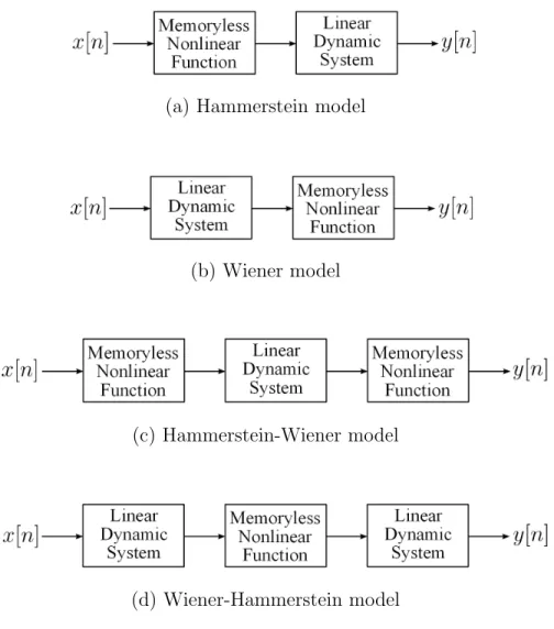
2-1 Fundamental Block-oriented Nonlinear Models . . . 45

3-1 Success Rates v.s. Increase of Degrees . . . 70

3-2 Success Rates v.s. deg_x(Finput), with deg (Ginput) = (4, 6) . . . . 71

3-3 Sensitivities of Bivariate Polynomial Factorization . . . 76

4-1 Hammerstein Model . . . 80

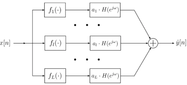
4-2 Parallel Hammerstein Model . . . 83

4-3 Equivalent Block Diagram for Figure 4-1 . . . 84

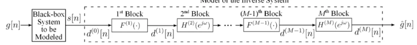
4-4 Block-oriented Cascade Model for the Inverse System . . . 89

4-5 Special Black-box System . . . 92

5-1 Modular Volterra System . . . 102

5-2 Modular Volterra System with Linear and Nonlinear Branches . . . . 104

5-3 Simpliﬁed Modular System with Linear Kernel . . . 107

5-4 Approximation of Cascade Volterra System . . . 108

5-5 Approximation of Modular Volterra System . . . 110

6-1 Pareto Fronts of Accuracy v.s. Number of Features Used . . . 144

(14)

(15)

List of Tables

4.1 Success Percentage of Parameter Estimation for Cascade Inverse . . . 98

5.1 Success Rates of Parameter Estimation for Modular Volterra System 113 6.1 Average Test Error Rates . . . 139

6.2 Average Numbers of Features . . . 140

6.3 Numbers of Features with Diﬀerent Binarization . . . 141

(16)

(17)

Chapter 1 Introduction

Parametric representations are widely used in signal processing for modeling both systems and signals. Examples of parametric representations include linear time-invariant ﬁlters with rational transfer functions that are parameterized by the coeﬃcients of the numerators and the denominators, bandlimited periodic signals that can be characterized by the fundamental frequency as well as the magnitude and phase of each harmonic, and stochastic signal models with parametric proba-bility distributions. Parameter estimation algorithms are usually needed for these representations to obtain the parameters from empirical observations or statistical information.

For certain classes of parametric models, the number of independent parameters is smaller than that of a natural parametrization of the model, which can enable an alternative and more compact parametrization. As an example, a class of two-dimensional (2D) finite impulse response (FIR) filters is the separable filters [3], the transfer functions of which satisfy H(z1, z2) = H1(z1)·H2(z2). If H1(z1) and H2(z2) are

of orders N1 and N2, respectively, then the total number of independent parameters1

is N1+ N2 + 1. If we consider the impulse response as a natural parametrization of H(z1, z2), then it has (N1+ 1)· (N2 + 1) parameters, and thus the parametrization

with H1(z1) and H2(z2) is more compact. As an example of signal representation,

1_{In fact, H}

1(z1) has N1+ 1 parameters and H2(z2) has N2+ 1 parameters. Since respectively

scaling H1(z1) and H2(z2) with c and 1/c leads to the same product, the number of independent

(18)

sparse signals have most elements as zero and can be eﬃciently characterized by the locations and values of the non-zero elements [4,5]. Moreover, low rank matrices are a widely used model in applications such as recommendation systems [6,7], background modeling for video processing [8, 9], and biosciences [10]; a low rank matrix can be parameterized by the non-zero singular values and the associated singular vectors from the singular value decomposition (SVD), which typically have fewer parameters than the total number of elements in the matrix.

As we can see from these examples, the reduction of independent parameters typically results from additional constraints on the parametric models, such as sepa-rability of 2D filters, sparsity of signals, and the low rank property of matrices. These additional constraints introduce dependence among the parameters in the natural representation, and therefore the number of degrees of freedom is reduced. From a geometric perspective, the feasible region of a constrained parametric model can be regarded as a manifold in a higher dimensional space associated with the natural parametrization. In signal processing, the reduction of independent parameters could lead to system implementation with higher efficiency, more compact signal representation, and efficient extraction of key information from high-dimensional data. As a class of constrained parametric models, composition structures typically have the form of systematic replacement of elements in an object with another object module. By using proper composition structures for system and signal representation, we can achieve the potential advantages of parameter reduction, modularity for hardware implementation, and the ability to form more sophisticated models that can represent significantly larger classes of systems or functions, which we will illustrate in later sections of this chapter.

There are diﬀerent types of composition with diﬀerent choices of objects and replacement approaches. As an example, function composition replaces the input variable of a function with the output of another function. It has been well-studied in theoretical and computational mathematics, spanning a wide range of topics such as polynomial composition [11–14], rational function composition [15, 16], and iterated functions that are generated by composing a function with itself multiple times [17,18].

(19)

Other types of composition considered in this thesis include operator composition and modular composition, where the latter refers to the replacement of each delay element in a system block diagram with another subsystem.

The remainder of this chapter is organized as follows. Section 1.1 reviews the diﬀerent types of composition structures and presents a few examples of the signal processing techniques that can be interpreted as a type of composition. After discussing the potential advantages of utilizing composition structures for system representation in Section 1.2, the focus and contributions of this thesis are summarized in Section 1.3. Finally, the outline of this thesis is proposed in Section 1.4.

1.1 Types of Composition Structures

1.1.1 Univariate Function Composition

Function composition generally refers to the application of a function to the result of another function. In particular, for univariate functions g(·) : A → B and f(·) : B → C, the composition (f◦ g)(·) is a function from the set A to the set C, which satisﬁes (f ◦ g)(x) , f(g(x)) for all x ∈ A. To ensure proper deﬁnition, the domain of the outer function f (·) should include the image of the inner function g(·).

Function composition can be interpreted from the following two equivalent perspectives:

• For any x ∈ A, we obtain v = g(x) and then obtain y = f(v). In other words, we replace the input variable of f (·) with the output of g(·).

• The function f(·) corresponds to an operator Flc that maps the function g(·) to

a new function (f◦ g)(·); similarly, the function g(·) corresponds to an operator Grc that maps f (·) to (f ◦ g)(·). The latter operator Grc is linear and named as

the composition operator or the Koopman operator [19], which has been studied in ﬁelds such as nonlinear dynamic systems and ﬂow analysis [20, 21].

The ﬁrst interpretation will be used in Sections 1.1.2 and 1.1.3, while we will focus on the second interpretation in Section 1.1.4.

(20)

Univariate function composition may serve as a convenient description for a number of signal processing methods and system structures. Frequency-warping [22, 23] replaces the frequency variable in the spectrum with a warping function and thus achieves non-uniform spectrum computation with the standard Fast Fourier Transform algorithm. Moreover, time-warping [24, 25] applies a warping function to the time variable and can be used for efficient non-uniform sampling. As an example of system representations with a composition structure, as shown in Figure 1-1, if we replace each delay element2 _{in a FIR filter F (z}−1_{) with another filter G(z}−1_{), then we}

obtain a modular filter with the transfer function as the composition of the transfer functions of the two filters F (z−1) and G(z−1). The design of such modular filters has been studied in [1, 2]. More detailed review on frequency-warping, time-warping, and modular filter design will be presented in Section 2.1 of this thesis.

(a): FIR ﬁlter F (z−1)

(b): Modular ﬁlter (F ◦ G)(z−1)

Figure 1-1: Modular ﬁlter with transfer function as (F ◦ G)(z−1) [1, 2]

1.1.2 Operator Composition

Operator composition has the same core idea as univariate function composition, with the only diﬀerence that functions are substituted by operators. In particular, for operators G{·} : A → B and F {·} : B → C, the composition of the two operators

2_{Here each delay element z}₋₁ _{(rather than z itself) is considered as the variable of the transfer}

(21)

is deﬁned as (F ◦ G) {·} , F {G {·}}.

In signal processing, a system can be considered as an operator that works on a set of signals of interest. Therefore, the cascade of two systems that respectively correspond to the operators G{·} and F {·} can be naturally represented by the operator (F ◦ G) {·}. The systems in the cascade can almost be arbitrary, as long as the system F{·} can take the output from the system G {·} as an input signal.

Cascade systems have been widely used and studied in signal processing. For linear systems, the cascade implementation of one-dimensional (1D) infinite impulse response (IIR) filters can improve the stability with respect to possible quantization errors in the filter coefficients [26]. For nonlinear systems, the block-oriented models are a useful and wide class of models that typically represents a nonlinear system by the interaction of linear time-invariant (LTI) blocks and nonlinear memoryless blocks [27], and the cascade nonlinear models are an important subclass of these block-oriented models. More detailed review on the block-oriented nonlinear models will be presented in Section 2.2.3 of this thesis.

1.1.3 Multivariate Function Composition

The composition of multivariate functions is a natural generalization of the univariate function composition. For multivariate functions f (v1,· · · , vR) and gr(x1,· · · , xd)

(1≤ r ≤ R), the function f(g1(x1,· · · , xd),· · · , gR(x1,· · · , xd)) is referred to as the

generalized composite of f with g1,· · · , gR [28]. Since there could be multiple inner

functions gr, this multivariate function composition gains additional ﬂexibility over

its univariate counterpart.

There are a number of important functions in signal processing that have the form of multivariate composition. As an example, two-level Boolean functions in the disjunctive normal form (DNF, “OR-of-ANDs”) or the conjunctive normal form (CNF, “AND-of-ORs”) serve as a useful classiﬁcation model and have wide applications in signal processing [29–31] and machine learning [32–34]. A Boolean function in DNF or CNF is a multivariate function with both the inputs and the

(22)

output as binary variables, which has the following form of composition:

ˆ

y = F (G1(x1,· · · , xd),· · · , GR(x1,· · · , xd)), (1.1)

where (x1,· · · , xd) and ˆy denote the input and output variables, respectively. For

DNF, the functions F (v1,· · · , vR) and Gr(x1,· · · , xd) (1≤ r ≤ R) in (1.1) are deﬁned

as F (v1,· · · , vR) = R ∨ r=1 vr, Gr(x1,· · · , xd) = ∧ j∈Xr xj, (1.2)

where each Xr (1≤ r ≤ R) is a subset of the index set {1, 2, · · · , d}, and the symbols

“∨” and “∧” denote the logical “OR” (i.e. disjunction) and “AND” (i.e. conjunction), respectively. For CNF, we swap the logical “OR” and “AND”, and the functions F and Gr (1≤ r ≤ R) are deﬁned similarly as follows.

F (v1,· · · , vR) = R ∧ r=1 vr, Gr(x1,· · · , xd) = ∨ j∈Xr xj. (1.3)

For simplicity, we refer to the individual functions F (v1,· · · , vR) and Gr(x1,· · · , xd)

as one-level Boolean functions, and thus the two-level functions are composition of the one-level functions.

The two-level Boolean functions in DNF and CNF have a number of beneﬁts. Since any Boolean function can be represented in DNF and CNF3 _{[34], these two forms have}

high model richness and are widely used in applications such as binary classiﬁcation [34] and digital circuit synthesis [35]. When the two-level Boolean functions are used in real-world classiﬁcation problems where each input and output variable corresponds to a meaningful feature, the variables selected in each subset Xr in (1.2) and (1.3) can

naturally serve as the reason for the predicted output; therefore, a two-level Boolean function model that is learned from a training dataset can be easily understood by the user, which may gain preference over black-box models, especially in ﬁelds such as medicine and law where it is important to understand the model [33, 36–38].

(23)

1.1.4 Modular Composition

The composition forms in previous sections focus on the replacement of the input information of a function or an operator by the output from another function or operator. In contrast, this section considers a generalization of composition by replacing elements in a system block diagram with identical copies of another system module, which we refer to as modular composition. In another perspective, the latter system module is embedded into the former system. For tractability, we focus on the example of replacing each delay element of a FIR ﬁlter F (z−1) in the direct form structure [26] with a time-invariant system G{·}, as shown in Figure 1-2.

(a): FIR ﬁlter F (z−1) in direct form structure

(b): Modular system

Figure 1-2: Embedding system G{·} into the FIR ﬁlter F (z−1) in the direct form structure.

The modular system in Figure 1-2 (b) is a natural generalization of the modular ﬁlter in Figure 1-1 (b), by allowing the system G{·} to be a general nonlinear module such as the Volterra series model [39, 40].

Now we consider the mathematical description of the modular composition process. For simplicity, we denote the set of signals of interest as S. The original subsystem G{·} is an operator that maps an input signal in S to an output in S, i.e. G{·} : S → S. After embedding G {·} in F (z−1), the modular system is another operator that maps from S to S. Thus, if we deﬁne the set of all operators from S to

(24)

S as

U , {H {·} : S → S} , (1.4)

then the system F (z−1) corresponds to a higher-level4 _operator F that maps from U to U . In summary, the modular composition process generally has the following mathematical description: the system within which we embed another module creates a higher-level operator, which has both its input and output as lower-level operators on the set of signals; we refer to this description as operator mapping, on which further discussion can be found in Appendix A.

1.2 Potential Beneﬁts of Composition Structures

for System Representation

As brieﬂy mentioned before, there are a number of potential advantages of the use of structures that can be interpreted as a type of composition for system representation purposes. In this thesis, we consider structures that have the following potential beneﬁts: parameter reduction, modularity for hardware implementation, and improved model richness, which are illustrated as follows.

• Parameter Reduction: If a given signal or system can be represented or approximated by a composition structure that has fewer independent parameters than the original signal or system, then this composition structure achieves representational compression or computational efficiency. As an example, a 2D FIR filter can be represented or approximated by a cascade of a pair of 2D FIR filters that have lower orders. If the cascade system retains the same order as the original 2D filter, then the cascade system typically has fewer independent parameters compared with the original 2D filter [41]. We will discuss the cascade approximation of 2D FIR filters in Chapter 3. Similarly, approximating a univariate polynomial by the composition of two

4_{The operator G}_{{·} works on the set of signals while F works on the set of operators, and}

(25)

polynomials with lower orders reduces the number of independent parameters and can potentially be applied to the compact representation of 1D signals, which is explored in [2, 42] and will be reviewed in Section 2.1 of this thesis. In addition, multiple layers of composition can achieve compact system structures by reducing the overall complexity. A class of examples is artificial neural networks that can be viewed as function composition of multiple layers, which is an efficient model for compact representations of a dataset and for classification tasks [43,44]; as suggested by [45–47], reducing the number of layers in a neural network may significantly increase the total number of neurons that are needed to have a reasonable representation.

• Modularity for Hardware Implementation: The modular systems in Section 1.1.4 use identical copies of a system module, which thus has a structured representation and achieves modularity. This modular structure can simplify the design and veriﬁcation for the hardware implementation with very-large-scale integration (VLSI) techniques [2, 48, 49]. As an example, we refer to a modular Volterra system as the system obtained by embedding a Volterra series module [39, 40] into a FIR ﬁlter, which will be studied in Chapter 5. • Improved Model Richness: Taking the composition of simple parametric

models of systems or functions may result in a new model that is able to represent a significantly larger class of systems or functions, i.e. the model richness is improved. As is discussed in Section 1.1.3, the one-level Boolean functions can model only a subset of all Boolean functions; in contrast, the two-level Boolean functions, which are the composition of one-level functions, can represent all Boolean functions if the negation of each input binary variable is available. Chapter 6 of this thesis considers algorithms to learn two-level Boolean functions from a training dataset. As another example for signal representation, the model of a bandlimited signal composed with a time-warping function can express signals that are in a significantly larger class than the bandlimited signals [24], which can enable efficient sampling methods for those

(26)

signals.

1.3 Focus and Contributions

Parameter estimation is a central problem for the utilization of the beneﬁts of composition structures for system representation. If we aim to use a composition structure to approximate a target system and signal, and if we choose the optimality criterion as the approximation error, then this performance metric is generally a nonlinear and potentially complicated function with respect to the parameters in the structure, which may make eﬃcient parameter estimation challenging.

This thesis focuses on parameter estimation for composition structures. Since an eﬃcient parameter estimation algorithm for general and arbitrary composition structures is unlikely to exist, this thesis proposes algorithms for the following classes of structures that have high importance for signal processing purposes: for the operator composition that corresponds to cascade systems, we consider the cascade approximation of 2D FIR ﬁlters and the block-oriented models for nonlinear systems; for modular composition, we propose the modular Volterra system; for multivariate function composition, we focus on algorithms to learn the two-level Boolean functions from a training dataset. We summarize the goals and the main contributions for each class of structures as follows.

• Operator Composition: As an example of cascade linear systems, we consider the approximation of a 2D FIR filter by the cascade of a pair of 2D FIR filters that have lower orders, which can achieve computational efficiency for spatial domain implementation. In the transform domain, the cascade approximation becomes approximate bivariate polynomial factorization, for which this thesis introduces new algorithms. Simulation results show that our new algorithm based on the idea of dimensional lifting of the parameter space outperforms the other methods in comparison. In addition, this technique can also be applied to the approximation of a 2D signal by the convolution of a pair of 2D signals with shorter horizontal and vertical lengths, which can result in

(27)

compact representation of 2D signals.

For cascade structures of nonlinear systems, we consider the block-oriented representations of discrete-time nonlinear systems, where the goal is parameter estimation using statistics or empirical observations of the input and output signals. In particular, we focus on two structures. The first structure is a Hammerstein model [50] that is the cascade of a nonlinear memoryless module followed by a LTI subsystem, where the nonlinear module is a weighted combination over a basis of known functions and the LTI subsystem has no extra constraints. This setup is more general than the LTI subsystems considered in existing literature on the Hammerstein model estimation, which typically are constrained to be FIR filters [51] or filters with rational transfer functions [52]. We generalize the two-step parameter estimation method in [52] from a finite-dimensional to an infinite-finite-dimensional parameter space. The second structure for nonlinear system is used for modeling a black-box nonlinear system by its inverse, where the inverse system is a cascade of multiple nonlinear functions and LTI subsystems. This second structure can be considered as a generalization of the all-pole signal modeling [26] by introducing nonlinear blocks.

• Modular Composition: The modular Volterra system is obtained by replacing each delay element in a FIR filter with a Volterra series module. If the Volterra series module has only the linear kernel, then the resulted modular system belongs to the class of modular filters in [1, 2]. In addition to modularity, the incorporation of nonlinear kernels in the Volterra series module has the additional benefit of capturing nonlinear effects and providing more flexibility over modular filters. In this thesis, we consider parameter estimation for the modular Volterra system using the statistical information between the input and output signals. In particular, we focus on the situation where the coefficients of the nonlinear kernels of the Volterra module have sufficiently smaller magnitude compared with those of the linear kernel, i.e. weak nonlinear effects. An estimation algorithm is provided by first obtaining the coefficients of

(28)

the linear kernel and then the nonlinear kernels, which is shown to be eﬀective by numerical evaluation when the order and the number of states (i.e. the maximum delay) of the system are not high.

• Multivariate Function Composition: In contrast to the above systems that have continuous-valued input and output signals, the two-level Boolean functions mentioned in Section 1.1.3 have binary input and output variables. Our goal is to learn two-level Boolean functions in the CNF or DNF [53] for classification purposes, with the joint criteria of accuracy and function simplicity. We propose a unified optimization framework with two formulations, respectively with the accuracy characterized by the 0-1 classification error and a new Hamming distance cost. By exploring the composition structure of the two-level Boolean functions, we develop linear programming relaxation, block coordinate descent, and alternating minimization algorithms for the optimization of the formulations. Numerical experiments show that two-level functions can have considerably higher accuracy than one-level functions, and the algorithms based on the Hamming distance formulation obtain very good tradeoffs between accuracy and simplicity.

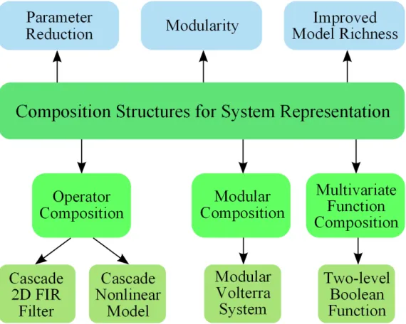
In summary, Figure 1-3 shows the framework of this thesis.

1.4 Outline of Thesis

The remainder of this thesis is organized as follows. After a high-level review of the related concepts and background in Chapter 2, we consider each class of systems as mentioned above. For cascade structures that correspond to operator composition, the cascade approximation of 2D FIR ﬁlters is presented in Chapter 3, and the block-oriented cascade models for nonlinear systems are studied in Chapter 4. For modular composition, the modular Volterra systems are introduced in Chapter 5. For multivariate function composition, learning two-level Boolean functions in CNF or DNF is considered in Chapter 6. In each chapter, the concrete form and the

(29)

(30)

applications of the composition structures are presented, the parameter estimation problem is formulated, related existing work is reviewed, new parameter estimation algorithms are proposed, and simulation results are shown to evaluate the algorithms. Finally, conclusion and future work are provided in Chapter 7.

(31)

Chapter 2 General Background

This chapter provides a brief review of fundamental concepts and existing works on a few important topics that are related to this thesis. Some of the reviewed techniques and system structures will be further discussed in later chapters, where a more detailed review will be presented for speciﬁc problems. Section 2.1 of this chapter reviews existing signal processing techniques and system structures that can be interpreted as a type of composition. Since both the Volterra series [39] and the block-oriented models [27] for nonlinear systems will be heavily used in later chapters of this thesis, Section 2.2 provides a brief review on these models for nonlinear systems and the associated parameter estimation approaches.

2.1 Systems with a Composition Structure

First, we review the work [2] that is the closest work to this thesis. In [2], Demirtas introduces the ﬁrst work that systematically studies function composition and decomposition for signal processing purposes, which are applied to the interpretation of existing techniques and the development of new algorithms, from both analysis and synthesis perspectives. The utilization of function composition and decomposition provides the beneﬁts of compact representation and sparsity for signals, as well as modularity and separation of computation for system implementation. In particular, there are three main focuses in [2], namely univariate polynomial decomposition, the

(32)

design of modular ﬁlters by frequency response composition, and the representation of multivariate discrete-valued functions with a composition structure, each of which will be reviewed as below.

• Univariate Polynomial Decomposition: Univariate polynomial decom-position generally refers to the determination of a pair of polynomials f (x) and g(x) so that their composition f (g(x)) equals or approximates a given polynomial h(x). Approximating a given polynomial h(x) by the composition f (g(x)) generally reduces the total number of independent parameters. Since the z-transform of a 1D signal is a polynomial, polynomial decomposition can be used for compact representation of 1D signals. A challenge with polynomial decomposition is the highly nonlinear dependence of the coefficients of h(x) on those of g(x). Practical decomposition algorithms are proposed in [2, 42, 54] and compared with existing works [12–14, 55], for both the exact decomposition where the given polynomial h(x) is guaranteed decomposable and the approximate decomposition where a decomposable polynomial is used to approximate a given indecomposable polynomial. These algorithms can work with either the coefficients or the roots of the given polynomial h(x) as the input information. As shown by [14], univariate polynomial decomposition can be converted to bivariate polynomial factorization, where the latter is related to Chapter 3 of this thesis. In addition to decomposition algorithms, sensitivity of polynomial composition and decomposition is studied in [2,56] by characterizing the robustness of these two processes with respect to small perturbations in the polynomials; the sensitivity is defined as the maximum magnification ratio of the relative perturbation energy of the output polynomial over that of the input polynomial. A method of reducing the sensitivity by equivalent decomposition has been proposed in [2, 56], which improves the robustness for polynomial composition and decomposition.

• Modular Filters by Frequency Response Composition: As mentioned in Section 1.1.1, modular ﬁlters are obtained by replacing each delay element in

(33)

an outer discrete-time filter with an identical copy of an inner filter module; the frequency response of the modular filter is the composition of the transfer function of the outer discrete-time filter and the frequency response of the inner filter module. The modular filter in [1, 2] can be potentially considered as a systematic generalization of the filter sharpening technique [57], which uses multiple copies of a low quality filter to improve the quality of approximation for a given specification. In particular, two choices of the inner filter module are considered in [2]: the first is a linear phase discrete-time FIR filter, and the second is a continuous-time filter. With the optimality criterion as the minimax error in the magnitude response, algorithms are proposed for the modular filter design for both choices above. The modular filter design will be further discussed in Section 5.2.

• Multivariate Discrete-valued Functions with a Composition

Struc-ture: The third focus of [2] is the composition and decomposition of

multivari-ate discrete-valued functions. Using proper composition can reduce representa-tional complexity and simplify the computation for the marginalization process, where the marginalization process has applications in topics such as nonlinear ﬁltering and graphical models in machine learning and statistical inference. In particular, the work [2] proposes a composition form for multivariate functions by introducing a latent variable that summaries a subset of the input variables. In this framework, a function f (x1,· · · , xn) is represented as ˜f (x1,· · · , xm, u)

where the latent variable u = g(xm+1,· · · , xn) (1 ≤ m < n). If the alphabet

size of u is sufficiently small, then representational efficiency is gained since the functions ˜f and g have fewer parameters than the original function f ; similarly, computational efficiency is achieved for marginalization. A generalization of the above composition form is proposed in [2], where a low rank approximation is used for a matrix representation of the multivariate function, which may also potentially reduce the number of independent parameters.

(34)

In addition to the topics that are explored in [2], there are a number of other techniques that can be interpreted from the perspective of composition structures. Here we list a few examples of such techniques, some of which have already been brieﬂy mentioned in Chapter 1.

• Time-warping and Eﬃcient Sampling: As brieﬂy mentioned in Section 1.1.1, replacing the time-variable of a signal f (t) with a function w(t) yields a composed function g(t) = f (w(t)), where w(t) is monotonic and can be considered as a time-warping function. If the signal f (t) is non-bandlimited, then a periodic sampling process will lead to information loss and cannot recover f (t) without additional information. However, for certain signals f (t), there may exist a proper time-warping function w(t) such that f (w(t)) becomes bandlimited, which thus enables periodic sampling without information loss. The work [24, 25] explores the signal representation technique with a proper time warping before periodic sampling, where the time warping function is also estimated from the input signal and aims to reduce the out-of-band energy before sampling.

• Frequency Transformation and Filter Design: A filter design problem can have the specification in a nonlinear scale of the frequency variable; as an example, the audio equalizer may have a logarithm scale specification [23]. If we convert the specification to a linear scale of frequency, then there are potential sharp ripples in the target frequency response where the frequency is compressed. This can lead to a high order of the designed filter and a lack of robustness in implementation. A possible solution to the problem above is the frequency warping technique [23], which approximates the nonlinear scale of frequency axis by replacing the delay elements in a filter with a proper system. This frequency warping process prevents the shape ripples in the target frequency response, leading to lower orders of the designed filters and higher implementation robustness. As briefly mentioned in Section 1.1.1, this idea of frequency warping has also been applied to the non-uniform spectrum

(35)

computation with the standard Fast Fourier Transform algorithm [22]. In addition to the above warping function that rescales the frequency axis, there are other frequency transformation functions that map the low frequency region to other frequency intervals; therefore, by the composition with a proper frequency transformation function, a prototype lowpass filter can be utilized to design a highpass or a bandpass filter with flexible choices of band-edges [58, 59].

• Eﬃcient Representation of Nonlinear Systems: For certain autonomous dynamical systems that have a nonlinear evolution on the state variables, there can be a simpliﬁed description of the system by utilizing proper function composition [60]. In particular, we consider an autonomous discrete-time dynamical system with the evolution as g : V → V where V ⊆ RN _{is the}

set of all possible state variables. If x[n] is the state variable at time n, then the system satisfies x[n + 1] = g(x[n]). For any observable (i.e. a function of the state variables) f : V→ C, we consider the Koopman operator G such that G {f} (·) = (f ◦g)(·), which is a linear operator that forms function composition. If we interpret f (x[n]) as the observation at time n, then G maps the function from the current state to current observation to the function from the current state to the next observation. For certain dynamical systems, the evolution of the state variables x[n] has a simplified description by using a special set of observables, which bypasses the potentially complicated nonlinear function g(·). This simplified description has the following steps [60]. First, we consider the eigenfunctions fk(x) of the Koopman operator G, namely

G {fk} (·) = µk· fk(·), 1 ≤ k ≤ K,

where µk are the singular values, and K can be either ﬁnite or inﬁnite. This

equation is named the Schr¨oder’s equation [61], which along with other similar equations involving function composition has been well-studied in mathematics

(36)

[18]. Then, with the assumption that the identical function1 _{I(x) = x is in the}

range of the function space spanned by fk(x), i.e.

x = I(x) = K

∑

k=1

vk· fk(x), ∀x ∈ V,

where vk (1≤ k ≤ K) are ﬁxed vectors in V, the evolution of the system can

be equivalently described in the following expansion

g(x) =G {I} (x) = G { _K ∑ k=1 vk· fk } (x) = K ∑ k=1 vk·G {fk} (x) = K ∑ k=1 vk·µk·fk(x).

This expansion of the state evolution g(·) can be considered as a simpliﬁed representation of the system, since the dynamic in the space of the observables fk(·) (1 ≤ k ≤ K) is linear; as a result, the state at any time n (n ≥ 0) with

the initial state x[0] at time 0 can have the following simple expression

x[n] = g[n](x[0]) =

K

∑

k=1

vk· µnk· fk(x[0]), n ≥ 0,

where g[n]₍_{·) denotes the n}th _{iterate of the function g(}_{·). The above expression}

converts the nonlinear and potentially complicated evolution of the state variables into a weighted combination of the ﬁxed functions fk(·), where the

weights has an exponential relationship with the time. In the study of the Koopman operator, the three elements µk, fk(·), and vk have the terminologies

of Koopman eigenvalues, eigenfunctions, and modes, respectively [60]. The estimation of these three elements is the critical step for utilizing the above eﬃcient representation of nonlinear systems. With various setup of available information, there have been a number of works on the estimation of the three elements or a subset of them, such as the generalized Laplace analysis [62,63] and the dynamic mode decomposition with its extensions [60, 64, 65]. In addition to

1_{Since the identical function has a vector output, we can consider each scalar element of the}

(37)

discrete-time systems, this representation technique with the Koopman operator has also been generalized to continuous-time systems [62, 66].

2.2 Models for Nonlinear Systems

Since nonlinear systems are defined by the lack of linearity, there is no unified parametric description for a general nonlinear system. In contrast, various models for different classes of nonlinear systems have been proposed. This section reviews three widely used models, namely the Volterra series [39], the Wiener series [67], and the block-oriented models [27].

2.2.1 Volterra Series Model

The Volterra series model [39, 40, 68, 69] is applicable to represent a wide class of nonlinear systems. For a discrete-time time-invariant system, the Volterra series model represents each output sample y[n] as a series expansion of the input samples x[n]: y[n] = H{x[n]} = ∞ ∑ k=0 H(k){x[n]} , (2.1)

where H(k)_{{·} is the k}th_{-order operator of the Volterra system, which satisﬁes}

H(k){x[n]} = ∑

i1,i2,...ik

h(k)[i1, i2, . . . , ik]· x[n − i1]· x[n − i2]· · · x[n − ik], (2.2)

where the ﬁxed discrete-time function h(k)_[i

1, i2, . . . , ik] is referred to as the kth-order

Volterra kernel. If the system is causal, the kernels h(k)[i1, i2, . . . , ik] are nonzero only

if all iq ≥ 0 (1 ≤ q ≤ k).

There are multiple perspectives to interpret the Volterra series model. If the system is memoryless, then the Volterra series recovers the Taylor series; therefore, the Volterra series could be regarded as a generalization of the Taylor series with memory eﬀects. While the Taylor series can represent a wide class of functions, the Volterra series can be considered as a representation of operators that map the

(38)

input signal to the output signal. The Taylor series may be inefficient and have slow convergence if there is discontinuity in the function or its derivatives; similarly, the Volterra series is more effective to model systems if the input-output relationship is smooth and if the nonlinear properties can be effectively captured in low order terms. The kth_{-order operator H}(k)_{{·} in the Volterra series model is k}th_-order

homo-geneous with respect to scaling of the input signal. In other words, if we replace x[n] by c· x[n], then the output term satisﬁes H(k)_{{c · x[n]} = c}k_{· H}(k)_{{x[n]}. The}

Volterra series model can be regarded as a generalization of the linear system; for a linear system, the ﬁrst-order Volterra kernel is the same as the impulse response of the system, and kernels of the other orders are all zero.

From another perspective with a dimensionally lifted signal space, the Volterra series represents the output of the nonlinear system as the summation across all the orders of the diagonal results from the multi-dimensional linear ﬁltering of the kernels and the outer-products of the input signal. More speciﬁcally, we can construct the outer-products of the input signal in the k-dimensional space as

˜ x(k)[n1, n2, . . . , nk], k ∏ q=1 x[nq]. (2.3)

If we ﬁlter this signal with the kth_{-order kernel h}(k)_[i

1, i2, . . . , ik] and then take the

diagonal elements, we obtain the term H(k)_{{x[n]} in (2.2). Finally, as shown by}

(2.1), the output signal y[n] is the summation of H(k){x[n]} across all orders k ≥ 0.

From this perspective, the kernel h(k)_[i

1, i2, . . . , ik] could be regarded as a generalized

impulse response in the k-dimensional space for the Volterra system. Moreover, it is clear that the output signal is linearly dependent on the kernels h(k)_[i

1, i2, . . . , ik].

By constraining both a finite order and a finite delay (i.e. a finite number of state variables), the Volterra model becomes simplified and more practical, which can be expressed as ˆ y[n] = K ∑ k=0 N ∑ i1=0 N ∑ i2=0 · · · N ∑ ik=0 h(k)[i1, i2, . . . , ik]· x[n − i1]· x[n − i2]· · · x[n − ik], (2.4)

(39)

where K and N are the highest order and the maximum time delay (i.e. the number of state variables), respectively. By increasing K and N in (2.4), this truncated Volterra series model can approximate a nonlinear system y[n] = HNL{x[n]} with any speciﬁed

accuracy, as long as the nonlinear system satisﬁes the following constraints [70]: • The operator HNL{·} is causal, time-invariant, continuous, and has fading

memory as deﬁned in [70];

• The input signal x[n] is upper and lower bounded.

Despite its high model richness, a disadvantage of the Volterra model results from the large number of parameters in the kernels. If we fix the maximum delay of the system, then the number of parameters in the kth-order kernel is exponential with respect to k. Therefore, these kernels may require sufficiently long observed signals in order to avoid overfitting for the parameter estimation.

The Volterra series model can also be applied to representing continuous-time nonlinear systems. For a time-invariant system, the output signal y(t) can be expressed in terms of the input signal x(t) and the Volterra kernels h(k)_(t

1, t2, . . . , tk)

in the form below:

y(t) = ∞ ∑ k=0 H(k){x(t)} , where H(k){x(t)} = ∫ · · · ∫ ( h(k)(t1, t2, . . . , tk)· x(t − t1)· x(t − t2)· · · x(t − tk) ) dt1dt2· · · dtk.

We can see that the summations in (2.2) for discrete-time systems are replaced by the integrations in the equation above for continuous-time systems.

A number of techniques have been developed to estimate the kernels in both the discrete-time and continuous-time Volterra models, with the tools of the higher-order correlations, orthogonal expansions, and frequency domain methods [71]. Here is a brief review on a few existing kernel estimation techniques. In addition to the following techniques, the Volterra series model can be reorganized into the Wiener series model [67] that is reviewed in Section 2.2.2, for which there are other kernel estimation approaches.

(40)

For a discrete-time Volterra system with a finite order and a finite delay, the output signal has linear dependence on the kernels. As a result, if the higher-order statistics [72] of the input and output signals are available, then the minimization of the power of the estimation error in the output can be formulated as a linear regression problem, and thus the kernels can be estimated by the least squares solution. Despite the simplicity of this approach, it may require heavy computation when the order or the delay is big. Generally, the kernels of different orders in the Volterra series are correlated with each other, and therefore all of the kernels need to be estimated simultaneously by solving a set of high-dimensional linear equations.

For continuous-time Volterra systems, the minimization of the mean squared error in the output involves integration equations that are generally challenging to solve directly. A special situation where the integration equations have a straightforward solution is Volterra series with kernels only up to the second order and with white Gaussian input signals [71]. An approach for general continuous-time Volterra kernel estimation is to expand the kernels on an orthogonal function basis and then estimate the expansion coeﬃcients [67,71], where the latter step can be achieved by approaches such as gradient-based techniques [73, 74] and pattern recognition methods [75]. As an alternative approach for kernel estimation, if we consider the Laplace or Fourier transform of the kernels, then the associated multi-dimensional transfer functions can be estimated with the higher-order spectra between the input and output signals [76,77], and eﬃcient transform algorithms can be applied to reduce the computational complexity [78].

2.2.2 Wiener Series Model

The kernels of the Volterra series can be reorganized in order to achieve mutual orthogonality. Here the orthogonality is in the statistical sense and considers the cross-correlation between diﬀerent terms in the series expansion of the output signal, where the input signal is a stochastic process with a speciﬁed probability distribution and autocorrelation properties. As a famous example, the Wiener series [67, 69, 79]

(41)

has the kth _term2 _W(k)_{{·} as a linear combination of kernels with orders no higher}

than k. If the input signal x[n] is a white Gaussian process with mean zero and variance σ2

x, then the kth Wiener term W(k){·} is orthogonal to any homogeneous

Volterra kernel H(m){·} where m < k, namely

E{W(k){x[n]} · H(m){x[n]}}= 0, for m < k and white Gaussian process x[n]. (2.5) Since W(m)_{{x[n]} is a linear combination of kernels with orders no higher than m,}

this orthogonality property (2.5) automatically guarantees that two Wiener terms with diﬀerent orders are orthogonal. For discrete-time systems, the Wiener terms of the lowest few orders have the following forms:

W(0){x[n]} = w(0), W(1){x[n]} = ∑ i1 w(1)[i1]· x[n − i1], W(2){x[n]} = ∑ i1,i2 w(2)[i1, i2]· x[n − i1]· x[n − i2]− σx2· ∑ i1 w(2)[i1, i1], W(3){x[n]} = ∑ i1,i2,i3 w(3)[i1, i2, i3]· x[n − i1]· x[n − i2]· x[n − i3] −3 · σ2 x· ∑ i1,i2 x[n− i1]· w(3)[i1, i2, i2], where w(k)_[i

1,· · · , ik] is named as the kth-order Wiener kernel [67, 79] and we assume

that each kernel is a symmetric function of its arguments, i.e. swapping any two arguments does not change the value of the kernel. From these examples, it can be observed that the kth _{Wiener term W}(k){·} includes the kth_{-order Wiener kernel} w(k)_[i

1,· · · , ik] as well as lower order kernels that are obtained by systematically

marginalizing w(k)_[i

1,· · · , ik] into dimension m, where m is smaller than k and has

the same parity as k. For a general Wiener term W(k)_{{·}, the coeﬃcients can be}

obtained from the Hermite polynomials [67, 79]. By replacing the summations with integrations, the Wiener series can also represent continuous-time nonlinear systems. Since the symmetry of the Gaussian distribution ensures that all odd order

(42)

moments are zero, the orthogonality property (2.5) holds if m and k have diﬀerent parity. When m and k have the same parity, the orthogonality property can be shown with the properties of the high order moments of Gaussian variables. As an example, we show the orthogonality property (2.5) for the situation when k = 3 and m = 1:

E{W(3){x[n]} · H(1){x[n]} } = ∑ j1 w(3)[j1, j1, j1]· h(1)[j1]· E { (x[n− j1])4 } + ∑ i2̸=j1 ( w(3)[i2, i2, j1] + w(3)[i2, j1, i2] + w(3)[j1, i2, i2] ) · h(1)_[j 1]· E { (x[n− i2])2 } · E{(x[n− j1])2 } −3 · σ2 x· ∑ i1,i2 w(3)[i1, i2, i2]· h(1)[i1]· E { (x[n− i1])2 } = ∑ j1 w(3)[j1, j1, j1]· h(1)[j1]· 3 · σx4+ 3· ∑ i2̸=j1 w(3)[j1, i2, i2]· h(1)[j1]· σ4x− 3 · ∑ i1,i2 w(3)[i1, i2, i2]· h(1)[i1]· σx4 = 0.

where we apply the property E {x4_{} = 3 · (E {x}2_})2 _{for a Gaussian variable x with}

zero mean.

With mutual orthogonality, each kernel can be estimated independently. There-fore, if we increase the order of the Wiener series, the lower order terms remain the same and do not need to be updated; however, we should notice that in general the mth-order Wiener kernel from W(m){·} does not fully determine the mth-order homogeneous kernel of the nonlinear system, since the term W(k){·} with k > m can

contribute to the mth-order homogeneous kernel. An approach for the estimation of the Wiener kernels is to further expand each kernel onto an orthogonal function basis and then to estimate the expansion coefficients [67, 69]. As an example, if we use the multi-dimensional Laguerre polynomials as the orthogonal basis for a continuous-time Wiener series model, then the estimation for each expansion coefficient has the following steps [67]. First, an auxiliary nonlinear system is created with the kernel as the Wiener G-functional applied to a function in the orthogonal basis. Then, the input signal is processed with this auxiliary nonlinear system. Finally, the expansion coefficient is the correlation between the output of this auxiliary system and the true system output. For this approach, the synthesis of the auxiliary systems may require excessive resources.

(43)

A widely-used approach for the Wiener kernel estimation is the Lee-Schetzen method and its variants [79–82], which uses the cross-correlation between the true system output y[n] and the delayed input signals. If the true system exactly satisﬁes the Wiener series model, then as is shown in [79], the coeﬃcients of the kth_-order

Wiener kernel can be estimated as follows

w(k)[i1,· · · , ik] = 1 k!· σ2k x · E {( y[n]− k−1 ∑ m=0 W(m){x[n]} ) · x[n − i1]· · · x[n − ik] } .

In addition, if the indices i1, i2,· · · , ik are mutually diﬀerent, then the result above

can be further simpliﬁed as [79]

w(k)[i1,· · · , ik] =

1 k!· σ2k

x

· E {y[n] · x[n − i1]· · · x[n − ik]} .

More rigorous analysis and deeper discussion about the applicability of the Lee-Schetzen approach can be found in [80, 81].

2.2.3 Block-oriented Models

The block-oriented models [27, 50, 67] represent a nonlinear system by the interaction between two types of blocks, namely the memoryless nonlinear functions and the linear time-invariant (LTI) systems. Compared with the Volterra series model, the block-oriented models typically compromise model richness to reduce the total number of independent parameters, which potentially simpliﬁes the process of system identiﬁcation. Another potential advantage of the block-oriented models is that each block in the structure may explicitly correspond to a physical property of the device or system that is modeled [27], which can result in improved model accuracy and physical interpretability.

As the most fundamental structures in this model class, the Hammerstein model [50] as shown in Figure 2-1 (a) is the cascade of a nonlinear memoryless block followed by a LTI subsystem, and the Wiener model [67] as shown in Figure 2-1 (b) is the cascade of the same blocks in the reverse order. Although relatively

Composition structures for system representation

Composition Structures for System Representation

by

Guolong Su

B.Eng. Electronic Eng., Tsinghua University, China (2011)

S.M. EECS, Massachusetts Institute of Technology (2013)

Submitted to the Department of Electrical Engineering and Computer

Science

in partial fulﬁllment of the requirements for the degree of

Doctor of Philosophy in Electrical Engineering and Computer Science

at the

MASSACHUSETTS INSTITUTE OF TECHNOLOGY

June 2017

c

⃝ Massachusetts Institute of Technology 2017. All rights reserved.

Author . . . .

Department of Electrical Engineering and Computer Science

May 19, 2017

Certiﬁed by . . . .

Alan V. Oppenheim

Ford Professor of Engineering

Thesis Supervisor

Accepted by . . . .

Leslie A. Kolodziejski

Professor of Electrical Engineering and Computer Science

Chair, Department Committee on Graduate Theses

Composition Structures for System Representation

by

Guolong Su

Abstract

Acknowledgments

Contents

List of Figures

List of Tables

Chapter 1

Introduction

1.1

Types of Composition Structures

1.1.1

Univariate Function Composition

1.1.2

Operator Composition

1.1.3

Multivariate Function Composition

1.1.4

Modular Composition

1.2

Potential Beneﬁts of Composition Structures

for System Representation

1.3

Focus and Contributions

1.4

Outline of Thesis

Chapter 2

General Background

2.1

Systems with a Composition Structure

2.2

Models for Nonlinear Systems

2.2.1

Volterra Series Model

2.2.2

Wiener Series Model

2.2.3

Block-oriented Models