Computational Light Routing: 3D Printed
Optical Fibers for Sensing and Display
The MIT Faculty has made this article openly available.
Please share
how this access benefits you. Your story matters.
Citation
Thiago Pereira, Szymon Rusinkiewicz, and Wojciech Matusik. 2014.
Computational Light Routing: 3D Printed Optical Fibers for Sensing
and Display. ACM Trans. Graph. 33, 3, Article 24 (June 2014), 13
pages.
As Published
http://dx.doi.org/10.1145/2602140
Publisher
Association for Computing Machinery (ACM)
Version
Author's final manuscript
Citable link
http://hdl.handle.net/1721.1/90397
Terms of Use
Creative Commons Attribution-Noncommercial-Share Alike
Princeton University / Disney Research Boston SZYMON RUSINKIEWICZ Princeton University and WOJCIECH MATUSIK MIT CSAIL
Despite recent interest in digital fabrication, there are still few algorithms that provide control over how light propagates inside a solid object. Existing methods either work only on the surface or restrict themselves to light dif-fusion in volumes. We use multi-material 3D printing to fabricate objects with embedded optical fibers, exploiting total internal reflection to guide light inside an object. We introduce automatic fiber design algorithms to-gether with new manufacturing techniques to route light between two arbi-trary surfaces. Our implicit algorithm optimizes light transmission by min-imizing fiber curvature and maxmin-imizing fiber separation while respecting constraints such as fiber arrival angle. We also discuss the influence of dif-ferent printable materials and fiber geometry on light propagation in the vol-ume and the light angular distribution when exiting the fiber. Our methods enable new applications such as surface displays of arbitrary shape, touch-based painting of surfaces and sensing a hemispherical light distribution in a single shot.
Categories and Subject Descriptors: I.3.5 [Computer Graphics]: Compu-tational Geometry and Object Modeling—Physically based modeling General Terms: Algorithms
Additional Key Words and Phrases: 3D printing, optical fibers ACM Reference Format:
Pereira, T, Rusinkiewicz, S., and Matusik, W. 2014. Computational Light Routing: 3D Printed Optical Fibers For Sensing and Display. ACM Trans. Graph. 28, 4, Article 106 (August 2009), 11 10.1145/1559755.1559763 http://doi.acm.org/10.1145/1559755.1559763
We thank the NSF grants CCF-1012147 and IIS-1116296, the DARPA grant N66001-12-1-4242, the Intel ISTC-VC and a Sloan Research Fellowship for funding.
Permission to make digital or hard copies of part or all of this work for personal or classroom use is granted without fee provided that copies are not made or distributed for profit or commercial advantage and that copies show this notice on the first page or initial screen of a display along with the full citation. Copyrights for components of this work owned by others than ACM must be honored. Abstracting with credit is permitted. To copy otherwise, to republish, to post on servers, to redistribute to lists, or to use any component of this work in other works requires prior specific permis-sion and/or a fee. Permispermis-sions may be requested from Publications Dept., ACM, Inc., 2 Penn Plaza, Suite 701, New York, NY 10121-0701 USA, fax +1 (212) 869-0481, or [email protected].
c
YYYY ACM 0730-0301/YYYY/14-ARTXXX $10.00 DOI 10.1145/XXXXXXX.YYYYYYY
http://doi.acm.org/10.1145/XXXXXXX.YYYYYYY
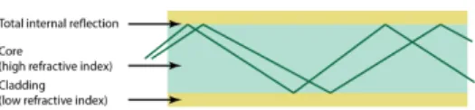
Fig. 1. Total internal reflection happens because of the higher refractive index in the core. This allows good propagation of light inside an optical fiber.
1. INTRODUCTION
Despite recent advances there are still few fabrication techniques and algorithms that let us control how light propagates inside a solid object. Existing methods design surfaces that reflect [Weyrich et al. 2009; Matusik et al. 2009] and refract light [Papas et al. 2011; Finckh et al. 2010] or restrict themselves to reproducing light dif-fusion in solid objects [Dong et al. 2010; Haˇsan et al. 2010]. We present automatic object design algorithms that, coupled with 3D printing, let us fabricate complex objects with embedded optical fibers. These fibers let us control light propagation in objects, en-abling novel display and sensing applications.
Printing optical fibers is made possible by modern multi-material 3D printers. We print two materials with different indices of refrac-tion (Figure 1). The core material, where light propagates, has a higher index. A low-index cladding material surrounds the core. The difference in indices causes total internal reflection, allowing light to propagate with low loss even after multiple bounces.
Recently Willis et al. [2012] have shown that many optical components can be custom printed including optical fibers. Using printed fibers they designed applications such as tangible displays in the form of chess pieces, custom sensors of mechanical motion and toys with dynamic eyes. However, the internal complexity of fiber volumes enabled by 3D printing, coupled with manufacturing constraints, led to a hard manual design problem.
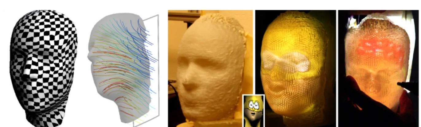
We propose an automatic fiber routing algorithm that accounts for these constraints. It routes light between arbitrary surfaces en-abling new applications of printed optical fibers. In entertainment applications, we created backlit face displays [Liljegren and Foster 1990]. In scientific visualization, we created a brain-shaped dis-play that let us visualize MRI data in context. In both cases, light from a micro-projector enters the fiber volume on a flat interface and is routed by the fibers to points on the surface (Figure 2). In addition, we prototyped sensing applications where fibers enable non-flat imaging surfaces. These include a touch sensitive display and a fiber hemisphere for BRDF acquisition. Finally, our algo-rithm could be used in photography applications in a design such
Fig. 2. We use 3D printing to fabricate objects with embedded optical fibers that route light between two interfaces. We use this pipeline it to create displays of arbitrary shape, such as this animated face. Given a parameterized output surface (left), our algorithm automatically designs the fibers (middle-left) to maximize light transmission. We use a micro-projector to input an image (inset) on the printed object’s (middle) flat interface, and it is routed to the surface (middle-right). We also present a painting application in which fibers are used for sensing and display. The light from a touch-sensitive infrared pen (right) is routed through the object to a camera.
as in Ford et al. [2013] to optimize the coupling between the curved surface of a lens and a sensor.
In this work, we characterize the capabilities and limitations of printing optical fibers (Section 3) including the advantages of us-ing different materials, how shape influences light propagation in the fibers and how to control the exiting light distribution. Next, we describe algorithms (Section 4) that take two arbitrary surfaces as input and design a volume of optical fibers to route light between them. Using our method, we design (Section 5) complex objects such as arbitrary shaped touch-sensitive displays and a hemispher-ical light distribution sensing component.
2. RELATED WORK
Fabrication. Fabrication has introduced the graphics community to problems of how to control the interaction of light with physical objects. Most recent work focuses on the surface of objects, in-cluding reproduction of reflectance [Matusik et al. 2009; Weyrich et al. 2009] or refraction [Papas et al. 2011; Finckh et al. 2010]. Other work designs objects with a custom interior structure, but this has been restricted to reproducing subsurface scattering [Dong et al. 2010; Haˇsan et al. 2010]. Our printed fiber volumes provide control of light propagation through total internal reflection in the interior of objects.
Recently, 3D printed optical components [Willis et al. 2012] in-cluding optical fibers were shown to have many applications in hu-man computer interaction such as motion sensors, volumetric dis-plays and toys with custom flat disdis-plays. We present new applica-tions of printed fibers enabled by using automatic design algorithms instead of manual design, such as display and sensing applications with non-flat surfaces. On the manufacturing end, we discuss the light transmission trade-offs involved in using different materials and techniques to control the angular distribution of exiting light.
Traditional manufacturing. Fiber imaging applications depend on fiber bundles which are traditionally manufactured in two steps. First each individual fiber is made in isolation. In some methods, they are constrained to constant cross-section. In other methods, they are even constrained to cylindrically symmetric cross-sections [Senior 1992]. Second these fibers are packed into a bundle which is then shaped. The process works by placing fibers together and applying heat to fuse them [Kociszewski et al. 1993]. At this point a simple parallel bundle is obtained, its shape can then be changed
by the simultaneous application of both heat and external forces. For example to create a taper, it’s possible to stretch the bundle at its end points resulting in thinning at the middle where the object can be cut. To create an image inverter, a rotation can be applied to the end points resulting in fibers in a helix shape.
Printed fibers avoid this global deformation step, by placing ma-terial voxels with different refractive indices directly in their final position. Printing enables bundles of much more complex shape, such as bundles with the shape of a face. While it is possible to start with a traditional bundle and grind it to any shape, it would be hard to control the fiber arrival angle. This is made easy with print-ing. Printing also has no limitation regarding cross-sections which can easily vary along the fiber. Currently these benefits come at the cost of impurities in the fibers, but most important not perfectly flat interfaces between core and cladding resulting from voxel quanti-zation which introduces light loss.
Inter-surface mapping. Given input and output surfaces, our routing algorithm creates fibers to connect them. There are a vari-ety of methods for morphing surfaces [Gomes et al. 1998]. While these morphing techniques create a sequence of intermediate steps through time, our approach can be seen as morphing through space. Our work differs from previous morphing methods because we are mostly interested in properties of the fibers themselves, such as cur-vature. In addition, we have to handle spatial manufacturing con-straints such as keeping fibers from getting too close.
We solve this 3D geometric problem using variational methods [Duchon 1977]. This approach has been used for other geomet-ric problems including surface design [Moreton and S´equin 1992] and deformation [Sorkine et al. 2004]. [Turk and O’Brien 1999] use thin-plate implicit functions to create a smooth morphing be-tween two surfaces. Techniques more similar to our work include [Botsch and Kobbelt 2005], who used triharmonic functionals for smooth shape deformation, and [Jacobson et al. 2012], who also used higher-order functionals for shape deformation. In our work, we use triharmonic functionals to have better control and continu-ity of curvature at the boundary conditions. In addition, we propose other objective terms to represent manufacturing limitations such as the minimum fiber spacing.
Fig. 3. Comparison of fiber designs with different materials. For all de-signs, light is strongest when the camera direction is aligned with the sur-face normal. On the left, VeroBlack cladding transmits no light. On the right, TangoPlus as cladding shows good transmission in the fiber direc-tion but also lets light pass even from other direcdirec-tions since it is transpar-ent. This is a problem since leaked light from one fiber may be captured by other fibers. Support material as cladding (middle-right) absorbs some leaked light which reduces cross-talk. Even lower cross-talk can be achieved with a 3 material design (middle-left) by surrounding support cladding with VeroBlack. While no leaking occurs, the resulting transmission is very low. On the back, a laptop screen feeds white light into all these fiber bundles.
3. FIBER FABRICATION
In this section, we describe different fiber designs with which we have experimented. These include the use of different materials (Section 3.1) and cross-section geometries (Section 3.2). We also include an analysis of the fiber’s field of view and how to improve it (Section 3.3). Finally, we measure how transmission varies with length and curvature (Section 3.4). The capabilities and limitations of fiber printing will guide the design of our algorithm (Section 4).
3.1 Choice of materials
An optical fiber is composed of two parts with different materi-als (Figure 1). The core is chosen to have a high refractive index, while the cladding has a low index. Most of the light propagation occurs in the core, with the light bouncing back when it hits the cladding due to total internal reflection. When designing optical fiber volumes for 3D printing, an important question is the choice of materials for core and cladding. In this subsection, we detail our experiments with different material combinations. For all experi-ments and applications in this work, we fabricated fibers using a Objet Connex 500 multi-material 3D printer.
We classify printed fiber designs according to different proper-ties. The ones that depend on material selection are effective light transmission, cross talk between fibers and numerical aperture. The effective transmission depends on how absorbent are the core and the cladding and how much light is internally reflected. Cross-talk occurs when light crosses the fiber walls into a neighboring fiber. It is caused by irregularities on the fabricated fiber walls, but also de-pends on how much of the leaked light is absorbed by the cladding. The numerical aperture is the range of incident angles that lead to total internal reflection. Incident rays that are outside this accep-tance angle range will mostly cross the fiber wall and leak. Numer-ical aperture depends mostly on the two refractive indices nco, ncl and is given by the following formula: sin(θmax) =pn2co− n2cl where θmaxis the angle of incidence with respect to the fiber axis. The acceptance angle is identical to the exiting angle of light from a fiber, which we will also call its field of view.
Similar to [Willis et al. 2012], we chose VeroClear as the core. This is a transparent and colorless material with a high refractive index (1.47). We also experimented with FullCure 720, which has similar refractive index but has a yellowish color. The cladding ma-terial should have a lower refractive index. We experimented with air as cladding (Figure 4) and also with different printer materi-als (Figure 3). Both TangoPlus (a clear flexible material with index
Fig. 4. Air cladding fibers have 180 degree field of view and excellent transmission, but they are impractical since support material is added be-tween the fibers during printing. This support material is very hard to clean for the intricate fiber geometries used in this work. From left to right, we see light imaged from increasingly grazing angles. On the back, a laptop screen feeds light into the bundle. At extreme right, we show the hexago-nal cross-section at the base of our fibers. This shape improves tiling of the input image plane with no observable loss in fiber transmission.
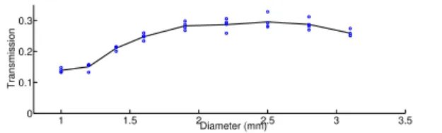
1 1.5 2 2.5 3 3.5 0 0.1 0.2 0.3 Diameter (mm) Transmission
Fig. 5. Transmission as a function of cross-section diameter (mm) mea-sured for a fiber of 8 cm of bending radius. Multiple conflicting diameter-related factors influence transmission including number of light bounces and incidence angle resulting in a sweet spot.
1.42) and the printer’s support material work well as cladding. Sup-port material absorbs more light, leading to fibers that are more re-silient to leaking. For this reason, we follow [Willis et al. 2012] and choose support as cladding. Both TangoPlus and support material have similar numerical aperture equivalent to a θmaxof 25 degrees.
3.2 Geometric factors
In this section, we describe our experiments with cross-section ge-ometry and core/cladding diameter ratio. We experimented with three different cross-sections: circle, square and hexagon. The square cross-section does not work. To our surprise, both circle and hexagonal fibers showed similar transmission. We chose to use hexagonal fibers because the hexagon tiles the plane well, leading to a larger area dedicated to the core of fibers. Circular sections always have extra cladding spaces due to tiling limitations. In addi-tion, hexagonal fibers reduce the number of mesh triangles needed to represent the geometry. This is a mundane, but practical, concern since printer software cannot handle models with very large trian-gle count. Besides cross-section geometry, the usable area also de-pends on the core/cladding ratio. Ideally, we would like to make the core very small and the cladding even smaller, but we are limited by the printer resolution. Most of the results shown in this work have a core diameter around 1mm and cladding spacing (distance be-tween neighboring fibers) around 0.15 mm. Our experiments with cladding spacing down to 0.05 mm failed because this size is very close to the printer resolution (0.042 mm in the x or y direction).
We have measured how fiber transmission varies with cross-section diameter (Figure 5). For this experiment, we restricted our-selves to circular cross-sections and printed fibers in an s-shape with 8 cm bending radius in each arc (more setup details in subsec-tion 3.4). We printed this fiber ranging in diameter from 1 to 3.1 mm. Multiple conflicting factors influence transmission. A larger diameter results in fewer light bounces and therefore less light loss. However, a larger diameter often results in bounces at a larger
inci-Fig. 6. Comparison of the transmission of 90◦turn fibers with varying curvature radii for both support and TangoPlus cladding. The radius of cur-vature of the top fibers is 5 cm.
dent angle which brings more loss. This is because the fiber curva-ture becomes non-negligible. Overall, transmission seems to vary only up to a factor of 2 due to diameter which is a much smaller impact than the one we observe from fiber bending and length. Yet these measurements reveal a sweet spot around 2.5 mm. We leave as future work determining how this sweet spot changes with fiber curvature and length.
3.3 Field of view
As seen in Figure 3, the limited exiting angle of a fiber has large im-pact on its use for display purposes. It constrains the field of view to the directions which are approximately aligned with a pixel’s sur-face normal. In this section, we discuss different ways to control the exiting light distribution with angle by making changes to the fiber ending. A solution to this field of view problem for flat displays is to use planar diffuser sheets, but this solution does not extend to ar-bitrarily shaped objects. After a few experiments, we chose to use a layer of diffuse white paint, which results in a 180 degree field of view. We experimented with applying white diffuse paint using spray cans and an air-brush. The air-brush provided finer control of the thickness of the applied layer of paint. This is important be-cause the thicker the paint the more diffuse the appearance, but also the less light is transmitted.
Our first attempt at a diffuser was adding a layer of support ma-terial to the fiber endings. We also attempted to increase scattering by appending heterogeneous endings: small dithered combinations of support and VeroClear or TangoPlus and VeroClear. All these so-lutions failed to increase the field of view by a significant amount. Next, we printed small lenses at the end of the fibers. The lenses do extend the field of view by some small angle because rays that arrive outside the accepted angle range are mapped inside. How-ever, some of the rays that were already accepted are bent to angles outside this range and therefore not transmitted. The net result is that from larger viewing angles only half a pixel is lit. We also ex-perimented with using a layer of a white diffuse printer material: VeroWhite. While it averages the angular light distribution well, it also introduces some spatial blur due to subsurface scattering. After all these experiments, we settled on using white paint for diffuser.
In conclusion, we manufacture our fibers using the following de-sign: VeroClear for core and support for cladding, hexagonal cross-section and white paint as diffuser.
3.4 Bending loss
In this section, we present an experimental evaluation of printed fibers. Light leaking is worse the higher the curvature. In our ex-perience, short fibers with curvature radius of 5 cm or larger can
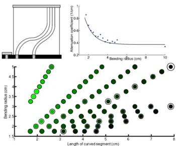
Fig. 7. We measure how fiber transmission varies as a function of cur-vature and length. Our setup consists of multiple fibers in an s-shape of constant curvature that continue into a straight segment (top-left). We fit an offset exponential (top-right) to describe the fiber attenuation coefficient (1/cm) as a function of the bending radius (cm). On the bottom, we show our measured transmission values (shown in green) as a function of bend-ing radius and length of its s-segment. The ratio of the radius of each two concentric circles is the measurement’s relative fitting error.
transmit incident light very well while fibers with curvature radius smaller than 1 cm carry almost no light. Figure 6 shows the trans-mission of 90 degree turn fibers with varying curvature radii. Even though the length of the fibers is larger the larger the radius, we can see that loss due to curvature dominates in this example.
To measure fiber attenuation, we printed fibers in s-shapes (Fig-ure 7). We also extend them by a straight segment so that many fibers have the same height. We can then focus a camera at this height making simultaneous measurements of multiple fibers with a single photo. Both arcs of the s-shape have the same radius. For each radius, we vary the arc angle resulting in varying total length but keeping the height fixed.
We measured two of these sets of fibers. The first set had a height of 6 cm and 6 radii values ranging uniformly between 1.75 to 3 cm. For each of these radii, we measure 7 different arc an-gles (28◦, 36◦, 45◦, 51◦, 60◦, 67◦, 75◦). The second set had a height of 7 cm and 8 radii values ranging uniformly between 3.25 to 5 cm. For each of these radius, we measure 4 different arc angles (15◦, 28◦, 36◦, 45◦). Notice that low angle values were avoided to guarantee that there is no line of sight between the pixel on the laptop screen and the camera.
We perform the transmission measurements using an LCD screen as input. The two fiber volumes are placed on the laptop screen which is all black except for gaussian blobs at the fiber po-sitions (Figure 7) top-left. These gaussians reduce aliasing caused from alignment problems. More light exits the fiber along its axis direction, this can cause problems due to slight off axis measure-ments. We use a transparent diffuser sheet (drawn in gray) to smooth the angular light distribution before measuring. We man-ually select the center and radius of each fiber in a high-dynamic range image and add the contribution of all pixels to achieve the final intensity value. The same process is performed for the screen pixels without any fibers on them (Figure 7 top-right). We simply
Fig. 8. Light propagation inside a poorly designed object cross-section. Since we are imaging from the side what we actually observe is scattering along the volume. While some light arrived at its destination even for com-plex routes, much light is leaking and scattering through the volume. The middle image also shows how more leaking happened at a high curvature region. We see how many light rays escape along the tangent direction.
place the diffuser sheet directly on the screen to get a measurement of the input light.
We assume the attenuation coefficient only depends on the bend-ing radius R. iout = iinexp(−α(R)l) where l is the length of a segment of constant radius in cm. Each measurement is not only influenced by the coefficient associated with its bending radius, but also by the straight segment loss. We performed two fittings to this data. First we assume α(R) = a + b exp(−cR). This exponential decrease of attenuation has been commonly observed both in theory and practice with traditional optical fibers for both fibers with di-ameter comparable and larger than light’s wavelength [Gloge 1972; Senior 1992]. We find α(R) = 0.37 + 2.5 exp(−1.1R), where at-tenuation is measured in cm−1and 0.37 corresponds to the straight fiber attenuation. This gives us a mean relative error of 15% and 68 of the 74 data points have relative error less than 33%. While this error is non-negligible, these fitting results support the exponential attenuation model with length and the exponential decrease of α. Figure 7 shows the transmission of the curved part of our measured fibers where brighter green means higher transmission. These are compensated measurements where the loss of the straight segment was estimated. The length axis measures only the curved part of each fiber. We plot two concentric circles for each measurement, the ratio of their radius is our model’s relative fitting error.
Second, we drop any hypothesis on α(R) and fit 15 bending at-tenuation values. Mean relative error decreases to 10% and now 68 of the 74 data points have error less than 20%. Figure 7 shows both the exponential model in black and the 15 attenuation coefficients in blue. We chose to plot the straight fiber attenuation coefficient as a point at radius 10 cm; this value is actually at infinite radius.
All these measurements confirm that transmission is greatly re-duced as the bending radius decreases which motivates our algo-rithmic decisions in the next section.
4. FIBER ROUTING
In theory, fibers carry light with no loss because of total internal re-flection. In practice, however, limited printer resolution introduces a minimum spacing between neighboring fibers and printer voxel quantization introduces surface irregularities that cause light to leak while propagating (Figure 8).
In this section, we present an algorithm to design fibers to route light to a user provided surface. We present different objective func-tions and design constraints that enable the automatic design of complex bundles to route light. Our algorithm receives two parame-terized surfaces as input and creates fibers to connect them. It maxi-mizes light transmission by minimizing fiber curvature. In addition, it maximizes fiber separation and constrains fibers to arrive orthog-onal to the input/output surfaces and conform to the user provided
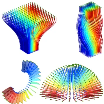
Fig. 9. Sample results show curvature optimized routes while respecting user provided parametrization constraints. The input and output surfaces can be arbitrary as shown in these cylinder and sphere routings.
Fig. 10. On the right, fibers generated by minimizing the thin-plate energy resulting in higher curvature in concentrated regions. On the left, minimiz-ing the third derivative energy which results in more uniform curvature. Plots display color coded curvature at different scales.
parameterization. We also show how to incorporate additional de-grees of freedom into our optimization by automatically selecting a parameterization of the volume’s flat interface (Subsection 4.3).
We propose an implicit formulation for the routing problem. Our algorithm receives as input both an input and an output surface, together with their u, v parameterizations. It then calculates u, v coordinates for every point in space by solving a variational prob-lem. Each fiber can be seen as the set of points in space that have a given u0, v0coordinate — in other words, a level set. In our current formulation, we solve for both u and v as separate optimization problems, so from now on we will only discuss u.
Figure 9 shows sample results of our algorithm for motivation. The green and blue points represent the input and output surfaces which can be arbitrary. We will denote the base by B and the tar-get surface by Q. Each input point has an associated u coordinate, which we denote by g(x). The algorithm extends these coordinates to all free space (displayed here as color).
The input parameterization serves as a hard constraint during op-timization. We impose the additional hard constraint that the fibers arrive orthogonal to the surfaces. Every time light crosses between
different media, there is a reflected and a transmitted ray. We con-strain the arrival angle to maximize the power of the transmitted ray. As an extreme case, rays arriving at very high angles would be internally reflected and no light would exit the desired surface. This angle constraint can be achieved by constraining the derivative of u(x) in the direction of the normal n(x). Notice that this normal need not be the true normal of the surface. For instance, when rout-ing complex models, we replaced it by smoothed normals, which still keep the arrival angle low but are less constraining.
Our objective function includes two different volumetric design goals: curvature C(u) and compression K(u). We formulate these objectives in the following quadratic program:
minimize u C(u) + wkK(u) subject to u(x) = g(x), x ∈ Q ∪ B, ∇u(x) · n(x) = 0, x ∈ Q ∪ B., (1) 4.1 Curvature term
As we have shown in the previous section, both fiber curvature and length influence transmission. Yet we observe, while solving our arbitrary surface routing problem, that high curvature is often the main cause of high loss (Figure 6). This is partly due to the fiber end points being hard constraints in our formulation. For simplicity, we chose to minimize fiber curvature and we leave as future work optimizing actual fiber transmission.
We would like to obtain a set of fibers that has minimum curva-ture. However, the expression for curvature is non-linear in u. It in-volves the product of second and first derivatives. We solve instead linear proxies to curvature that depend on derivatives. We experi-mented with minimizing second derivatives (thin-plate energy):
Z u2 xx+ u 2 yy+ u 2 zz+ 2u 2 xy+ 2u 2 xz+ 2u 2 yz (2) but chose to use third derivatives instead:
C(u) = Z u2 xxx+ u 2 yyy+ u 2 zzz+ 3u 2 xxy+ 3u 2 xxz+ · · ·. (3) Here the subscripts denote partial derivatives. The thin-plate energy resulted in fibers that were mostly straight but had high curvature in concentrated regions. As shown in Figure 10, the third deriva-tive energy better distributes curvature along the length of the fiber, avoiding these high curvature values. All results in this paper were generated using the third-derivative energy.
4.2 Compression term
If two fibers get too close to each other, the resulting volume might not be manufacturable. The reason is that there is a minimum width of cladding a printer can actually print. We use the term compres-sionto refer to many fibers coming together in a small area. In this section, we present an objective function to minimize average com-pression, or in other words, to maximize fiber spacing.
Let us start by considering the 2D case. In our implicit formu-lation, compression can be written as |∇u|. For example, when all fibers are going up then uyis zero and this constraint reduces to |du
dx|. This is exactly the number of fibers du per unit of space dx. We write our quadratic objective as K(u) =R u2
x+ u2y.
How to extend it to 3D space? One might consider maximizing the area of the fiber cross-section |∇u × ∇v|. However, this could still lead to thin walls between fibers in one direction. We simply minimize both |∇u|2and |∇v|2independently. This also maintains
Fig. 11. Effect of compression weight. In this example, we route fibers to a face. In the first row, we color-coded fiber endings with the max compres-sion over the fiber path. In the second row, we show the mean curvature over the fiber path. From left to right, compression weights of 0, 0.1 and 1. Not only, mean compression, but also mean curvature decrease. The drawback was that maximum compression and maximum curvature both increased.
the separable structure of our optimization problem. We can still solve two entirely separate problems one for u and one for v.
As an example of a result generated using our compression ob-jective see Figure 11, where we route light to a face. In the first row, we color-coded fiber endings with the max compression over the fiber path. In the second row, we show the mean curvature over the fiber path. As expected, we see that the mean curvature decreases with higher compression weights (more green). Surprisingly, the mean curvature also decreases from 0.038 to 0.026. This happened for all models we experimented with and can be understood by re-membering we are only optimizing an approximation to curvature. However, there are drawbacks. Maximum compression and maxi-mum curvature both increase from 1.65 to 1.70 and from 0.54 to 0.65 respectively. As a consequence, we usually keep low weights on compression to benefit from the decrease in mean values without hurting the maximum values much.
While adding these compression objectives gives us a useful de-sign tool to balance between compression and curvature, we would also like to add more degrees of freedom to the algorithm. In the next section we discuss how to jointly optimize the volumetric rout-ing and the base parameterization.
4.3 Base layout
So far we assumed the user provided parametric coordinates for the surface and the base. For some applications such as shape displays, the user is usually not interested in any particular base parame-terization. This means that ideally the algorithm should be free to change this parameterization if this change results in more efficient routing. In this section, we describe how to incorporate this extra degree of freedom to improve routing. With this variation, our al-gorithm can automatically decide where to place the base and with which scale. It also allows for non-linear stretching of the base. The major drawback of changing the fiber cross-section non-uniformly at the base is decreasing the input energy of some fibers and there-fore the display’s dynamic range. For all points on the base surface, we replace the constraint u(x, y) = g(x, y), where g was fixed, by a linear combination of basis functions:
u(x, y) =X i
αihi(x, y). (4)
Fig. 12. By optimizing the base parameterization jointly with fiber routing (right column), we obtain fibers with much less curvature (last row) and only slightly more compression (third row). On the top right, we show the base of the printed face model with its optimized fiber placement.
Fig. 13. We add a stretch energy term to keep the base from growing too large in cases where that minimizes curvature. On the top, we show the results with stretch weight 0.0001 and 0.001. The lower area weight result’s width was 40% larger. On the bottom, we show the base parameterizations for weight 0, 0.0001 and 0.001.
Fortunately, this is still a linear constraint. The only variables are the values of u and the coefficients αi. In our current implemen-tation, we chose a radial thin-plate spline basis hi(r) = r2log(r) centered at a grid of control points. In addition to these splines, we include the affine basis h1(x, y) = 1, h2(x, y) = x, h3(x, y) = y. Figure 12 shows the effect of using base layout. In the first row, we see a visualization of the unoptimized and optimized base pa-rameterization. In the second row, notice how the fibers on the right are more well behaved after their base positions are optimized.
The median of the maximum compression of each fiber increases slightly by 4.6%, while curvature showed large decreases. For ex-ample, the median of the mean curvatures decreased 39% and the median of the maximum curvatures decreased 29%. The mean compression of each fiber is visualized on the third row and the mean curvature on the last.
This method proved effective at finding smooth base parameter-izations. Moreover, we observed that these converge quickly when
experiment with other families of warps in order to capture high frequencies in the optimized base parameterization.
As we chose a family of thin-plate warps of the base parameter-ization, there is no guarantee it is a bijection. As happened in this example, the optimized base parameterization may assign the same u, v coordinate to multiple points on the base plane. This was a not a big problem since the resulting parameterization tends to be well-behaved around positions corresponding to fibers. The only step of the algorithm where not having a bijection was a problem was while sampling the base to grow fibers. Currently, we uniformly sample in u, v and solve for the corresponding x, y position to start the fiber. When there are multiple answers we found it adequate simply to choose the one nearest to the projected center of the mesh.
Base layout introduced an undesirable side effect when design-ing an inward lookdesign-ing hemisphere that routes light from a plane (Figure 14, right). Both our energies force the base to grow very large, since that reduces both curvature and compression (Figure 13, left). Since it is impractical to make these very large objects, we added an extra objective term to keep stretch low. This term works as a weak quadratic prior that pulls ux, uy, vx, vy towards their mean values on the target surface. Figure 13 shows how this term provides control over stretch. Both curvature and compression are volumetric terms, while stretch is an area term. We normalize all energies by volume and area respectively before adding them.
After the addition of the base layout constraints and the stretch energy term, our optimization problem is written below.
minimize
u C(u) + wkK(u) + wsS(u) subject to u(x) =X i αihi(x), x ∈ B, u(x) = g(x), x ∈ Q, ∇u(x) · n(x) = 0, x ∈ Q ∪ B., (5)
Using this algorithm, we routed and printed a few different sur-faces (Figure 14). The parameters used and some summary statis-tics of routing quality including curvature and compression are shown in Table I. Execution time, number of fibers and voxels can be found in Table II. In the next section, we show how these rout-ings behave when carrying light.
4.4 Path constraints
All routing examples discussed so far considered as constraints only the input and output surfaces. In fact, many important ap-plications of printed fibers [Willis et al. 2012] require additional constraints on the fiber’s path. For example, we may want fibers to guide light inside a character’s body to its eye or head. Alter-natively, some sensing applications of fibers may require avoiding other components such as buttons.
In this section, we show how additional linear equality or in-equality constraints can be added to our optimization formulation to represent these path constraints. They provide more routing con-trol to the user letting him specify relay points, bottlenecks, obsta-cles and even route around objects.
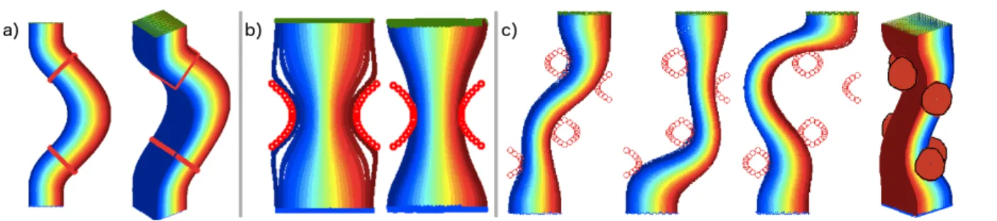
The simplest of these are relay points. If the user desires that a specific fiber u0, v0pass through a certain point in space x, we can simply identify which voxel contains the point and add the linear constraint u(x) = u0, v(x) = v0. Figure 16-a shows a case where relay points were used to bend the fiber 45◦to the right. This same
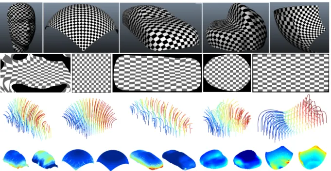
Fig. 14. Table of routing results. First row, the input parameterized mesh. Second row, the optimized base parameterization. Third row, randomly selected fibers. Fourth row, for each model we show mean curvature and mean compression per fiber.
Table I. Routing statistics. Each provided statistic is first a mean or max operator over each fiber’s path, followed by a median or max over all fibers.
Compression / Median of Max of Median of Max of Median of Max of
Bundle Area Weight Mean Curv Mean Curv Max Curv Max Curv Max Compr Max Compr
Face 0 / 0 0.022 0.072 0.073 1.05 1.16 1.55
Car 0.001 / 0.001 0.029 0.079 0.067 0.369 0.88 1.48
Brain 0.001 / 0.001 0.027 0.046 0.073 0.191 1.0 1.4
Inward 0 / 0.001 0.029 0.058 0.071 0.349 1.5 2.5
Sphere 0.01 / 0.001 0.013 0.034 0.022 0.838 0.94 1.40
Fig. 15. Routing around objects.
case highlights limitations of our implicit method: for bending an-gles larger than 60◦the resulting red fibers extended horizontally all the way to infinity, failing to connect input and output surfaces. Equality constraints can also be used to route fibers around an object (Figure 15). This was accomplished by identifying the co-ordinates of the two middle fibers, let’s say u0, u1, and adding the linear constraint u(x) = .5(u0+ u1) to on or more middle points. While equalities are useful, we found them to be rather limited. The problem is that in other settings, we just don’t know a priori the coordinate value of a point in space. For example, we experimented with routing through a bottleneck (Figure 16-b) using equality con-straints by setting the left wall’s coordinate to 0 and the right’s to 1. This led to very high curvature fibers since the leftmost and right-most fibers stuck to the walls. We found inequality constraints to
be much more expressive. By adding wall constraints u ≤ 0 to the left and u ≥ 0 to the right, we can achieve a low curvature fiber that fits in the bottleneck.
As a final example, we route fibers though multiple obstacles (Figure 16-c). Ideally, we would have a forbidden region con-straint. However, this is essentially an ’or’ concon-straint. At the ob-stacle points, u should be either less than 0 or larger than 1 which is not a convex constraint. Instead, we request as input for each obstacle if the fiber bundle should go to its right or left. Different combinations give the user control over the routing. These obsta-cles also work in 3D. In Figure 16-c, we apply these constraints independently to u and v. Each obstacle can constrain u, v sepa-rately or both at the same time.
We attempted solving simple versions of routing using this non-convex constraint and a local optimization technique (interior point method). However, being a local method it fails to jump over ob-stacles and it simply gets stuck to whichever left/right combination it was initialized with. As such a local method is not better than simply fixing sides.
4.5 Implementation details
We solve our optimization problem by discretizing u into a grid and using finite differences to approximate all derivatives. This
Fig. 16. Routing with constraints. Relay points (a) can be added to constrain the path of individual fibers using equality constraints. Bottleneck constraints can be implemented with equality constraints but this may lead to low quality paths (b-left). We used inequality constraints to achieve a low curvature routing through a bottleneck (b-right). Multiple obstacles (c) can be specified simultaneously in both 2D and 3D.
lution has one variable for each grid cell. Fortunately, since we are searching for very smooth fiber routings, small grids are suf-ficient to capture these low frequencies. Our problem is a quadratic program with linear equality constraints. Therefore, it is efficiently solved with a sparse linear system obtained using Lagrange mul-tipliers. The only exception is when we use inequalities for path constraints. In this case, we use an interior point method. All our implementations were performed in Matlab.
We grow the fibers by integrating the curves from their initial po-sitions in the input surface along the tangent field t = ∇u×∇v. We chose integrating fibers for simplicity of implementation. A more robust solution would be to extract the isocurves using interpolation of the grid data. In practice, we did not observe significant drifting even with this simple integration solution.
To create the final mesh, we create hexagonal cylinders for each fiber. The remaining question is choosing the cross-section orien-tation and shape at each point. Since ∇u, ∇v might not have the same norm and might not be orthogonal, our fibers have anisotropic cross-sections. We observed very small loss in transmission for small deviations from uniform cross-section. This justifies not im-posing additional cross-section uniformity constraints which would hurt other objectives.
In addition, when printing hexagonal fiber cross-sections, it is important to have a smoothly changing basis of the plane orthogo-nal to the fiber. We use ∇u to define one axis and choose the other one as ∇u × t, where t is the tangent. In fact, even when print-ing circular cross-sections, this smooth basis helps in connectprint-ing adjacent sections into triangles. For a given point on a fiber, after determining the local frame, we search for the 6 closest points, one in each of the adjacent fibers. With knowledge of these points we can create the local anisotropic cross-section without intersecting the neighboring cylinders.
Table II shows our algorithm runtime split in two stages: opti-mize and meshing. Optimization time is the solution of the linear system and depends only on the number of voxels. Meshing in-cludes time for fiber growth and mesh generation. The time it takes
Table II. Timings and sizes.
Bundle Voxels Fibers Optimize Meshing
Face 45k 5k 335s 289s Car 13k 7k 61s 391s Brain 11k 5k 43s 300s Inward 63k 2k 391s 97s Sphere small 48k 2k 960s 62s Sphere medium 48k 3.5k 960s 160s Sphere 48k 7k 960s 473s
depends only on the number of fibers. This is a big advantage of our implicit algorithm: the same optimized implicit function can be used to route fibers at multiple resolutions (spheres in Table II).
5. APPLICATIONS 5.1 Display
We can print displays of arbitrary shape by connecting projector pixels to surface elements. We use a micro-projector to input an image on the fiber bundle’s flat interface, and route light to the sur-face where it meets the diffuse paint for a complete field of view. Previous work on displaying animated content on surfaces can be divided in those that project from the outside [Raskar et al. 2001; Raskar et al. 2002] and those that project from the inside [Lil-jegren and Foster 1990]. When projecting from outside, a single projector is usually not enough for complex objects. Because not all points may be visible from a single viewpoint, multiple projec-tors are often used [Raskar et al. 2001]. This projection technique has a long history in entertainment including the singing heads at Disney’s Haunted Mansion and light shows on architectural mon-uments. The major drawback of all these techniques is that they require unobstructed clear air between the projectors and the ob-ject. For indoor settings, this prevents the viewers from touching or even getting close to the display. For outdoor settings, scatter-ing of the light rays caused by fog may reveal the technique. To avoid these limitations, [Liljegren and Foster 1990] project from the inside of the object using a wide-angle lens. Lenses restrict the maximum bending angle of light and also restrict the display ge-ometry to star-shaped objects. Our displays use fibers to carry light all the way to the surface pixel, enabling more light bending and more complex display shapes.
For each result in this section, the input parameterized mesh and the associated routing can be seen in Figure 14. The printed dis-plays and an evaluation of their point spread function and contrast are shown in Figure 18. This figure also shows the warped input image we project on the flat side and how it is seen on the display side. Table II shows the number of fibers for each display.
We printed a face display to project animated characters making different facial expressions. Figure 17 shows its appearance with varying content. It also shows the display seen from multiple view-points, which shows how the diffuse layer of paint worked well. In particular, from a fixed viewpoint, even points on the surface contour are visible. This display shows light bending by 90 degrees (side of face). It shows how we can achieve very concentrated point spread functions, which lead to sharp edges and adequate contrast. In fact, this face display shows how the contrast on the side of the face is actually better than in the front. The first reason is some of
Fig. 17. Face seen from different viewpoints and animation frames including open and closed mouths.
Fig. 18. Table of displays. First column, our printed displays. Second column, representative point spread functions imaged by lighting a few single fibers in the back. We show two versions of each PSF picture: a non saturated and a saturated version. The saturated image shows the dark tail of these distributions. Third and fourth columns, checkerboard images show how these objects can display sharp images but with low contrast. Fifth column shows the projected textures and the sixth column the result as seen on the surface.
the light that was to be routed to the side escaped through the tan-gent and arrived at the front of the face (see checkerboard images). Another reason is that some light enters the cladding instead of the core. These rays traverse the object and are not routed, eventually hitting the front of the face. We plan to investigate the use of masks to block this incoming light.
We also printed a half-sphere display that turns light by al-most 90 degrees. We projected a rotating globe animation. For this sphere, the layer of applied paint was not thick enough. As a result,
more light exists the surface in the normal direction than at grazing angles. This can be seen by the increased brightness in the middle of the globe picture. Notice that this cannot be fixed by calibra-tion, since it is a view dependent effect; it could only be fixed by a thicker layer of diffuse paint.
We printed a car display that allows us to dynamically change its content. We projected cars of different colors and blinking lights. While the image at the middle of this car display is very sharp (even for the 90 degree turns at the door), the front and back of the car
fibers was sharper when centering the projection there. This could be improved by placing the projector at a larger distance or even by printing displays with non-flat input interfaces.
Finally, our last display has the shape of a brain with half a lobe removed to reveal its inside. We use it to display volumetric f-MRI data. Each point on the surface of our display is assigned the color of the corresponding point in the MRI volume. This shows how our technique can handle even very concave display surfaces. However, this comes at the expense of dynamic range, since transmission of different fibers varies considerably. We show uncalibrated checker-board images and a manually calibrated MRI image which slightly improved the result. There are two reasons for the varying dynamic range of fibers. First, because of the concave region, the surface parameterization of the brain mesh is much less uniform than the other models (compare the pixel sizes on the left and right lobes). Second, fibers that arrive at the cutting plane took much more com-plex curved paths than other fibers (see Figure 14). The brain is the only result in this paper where we used intensity calibration.
We also printed simpler fiber volumes where both interfaces are flat. Using fibers, we prototyped merging two images where we route the light from the physical displays to the final display plane (Figure 19). The top image shows a tiling of the two input images. The black band cannot be seen from this viewpoint. It is currently not seamless because the relayed image is also darker and blurrier. In future work, we would like to use fibers to route light around an object making it ’invisible’ from a given view direction.
The content for the face, sphere and car displays was gener-ated by positioning the display surface mesh near a moving or deformable mesh and transferring the shading attributes at each frame. This process creates an animated texture that can be pro-jected at the object’s base. Notice that the parameterization used is not the user provided one, but instead the new mesh parameter-ization induced by the base layout optimparameter-ization. Both the car and face textures highlight these distortions. For the brain, we simply intersect the display surface with the volumetric image.
5.2 Sensing
While fibers can be used to carry light from a projector to a display surface, they can also be used to carry light in reverse. We designed two sensing applications of fibers: touch-sensitive painting on sur-faces and hemispherical light distribution acquisition.
Touch-sensitive painting. Simultaneous sensing and display through the same fiber can be challenging. Projected light is usu-ally much stronger, which compromises the signal to noise ratio of the sensing measurements. For interactive painting, we deal with this problem by sensing infrared light. It is important to use near-infrared, since our experiments showed our printed fibers are not capable of carrying wave-lengths farther from the visible spectrum. For our setup, we used a pen that has an LED at its tip. It emits light when pressure is applied to the tip, such as when touching the surface. The input light is then carried in the reverse direction and lights the appropriate pixel on the object’s flat side. While there is some leaking onto neighboring fibers, this was not significant. We have a camera placed near the projector with an infrared filter to detect which fiber was lit. The infrared filter worked well and the projector emitted almost no infrared light; as a result, the signal to noise ratio was extremely good. Both the camera and projector have to stay close to each other such that both fall inside the numerical
Fig. 19. The left image shows a tiling of the two input images. The black band is not seen from this viewpoint. It is currently not seamless because the relayed image is also darker. In the middle image, we move the tiling component. Notice how the black band is now very visible and the tent pole is not. The right image shows how a half-sphere fiber volume with no dif-fuser can be used as a fish-eye lens. It can implement complex projections; shown here is a stereographic mapping. Notice how nearby objects (a hand) are imaged through these fibers.
Fig. 20. Painting on a face using a touch-sensitive IR LED pen.
Fig. 21. Image of the hemispherical light distribution exiting different small material samples when illuminated by a directional light source. We use black cloth to mask the input material leaving only a small sample lo-cated at the center of the hemisphere (lower right). The angular light distri-bution is routed by the fibers to the camera’s focal plane. In the first row, white diffuse paper and white specular paper illuminated from two differ-ent directions (insets show enlarged images of the captured highlights). The next five images show specular highlights of anisotropic metal for varying light incidence angles and two orthogonal material orientations.
aperture of all fibers. This was not an issue in our setup with the face as a display. Figure 20 shows this system in action. We start with a skin color canvas and draw a red and white head band to-gether with a big yellow earring. Notice how the pen is detected even for fibers that curve 90 degrees. Painting on physical objects was previously explored with a head mounted display and a sep-arate haptic interface for detecting position of the pen [Agrawala et al. 1995]. Our setup allows displaying and sensing through the same object and only requires projectors and cameras.
Hemispherical light distribution acquisition. We designed a set of fibers to route light between a plane and an inward looking hemisphere. As a proof of concept, we applied it to capturing the angular light distribution coming from a material sample. This is an important component in BRDF acquisition. Our setup and re-sults are shown in Figure 21. Black cloth is used to isolate a sam-ple of three different materials including white diffuse paper, white specular paper and anisotropic metal. We light the material with a laser pointer from multiple directions and image the response on the flat side. No diffuser material is used for this application, since we do not need an extended field of view. In fact, we would rather have a shorter field of view. The images acquired by our setup can capture the shape of the different material highlights and their ori-entation. Our assembly provides good angular coverage at the cost of introducing some blur. We believe these qualitative results are promising. In future work, our transmission model could be used to calibrate the hemisphere allowing quantitative evaluation.
Besides sensing light, our first experiments suggest that it is also possible to use such a hemisphere to illuminate the material sample. We leave as future work a setup that can illuminate from any direc-tion on one hemisphere and capture from any direcdirec-tion in the other hemisphere, thus enabling full BRDF capture. This would build on prior work in no-moving-parts BRDF acquisition including sys-tems such as that of Dana [2001], which combined a parabolic mir-ror and beam splitter to allow BRDF acquisition without requiring either camera or light source to move around the sample. How-ever, this system was limited in its angular coverage. Ben-Ezra et al. [2008] built a BRDF measurement system based on LEDs placed on a hemisphere, using them for both illumination and sens-ing. While this allowed for BRDF acquisition with no moving parts and full angular coverage, the sampling rate was limited because of the need to place discrete LEDs on a hemispherical dome. Our 3D printed hemisphere-to-plane optical fiber assembly holds the po-tential for no-moving-parts, full-coverage BRDF acquisition, with an angular sampling rate limited only by the ratio of fiber width to overall printed hemisphere size.
Printed fibers should have additional applications in photogra-phy. As a very simple example, an outward looking sphere behaves as a fish-eye lens. It can implement complex projections with a pas-sive setup. Shown here, a stereographic mapping (Figure 19, right).
6. LIMITATIONS
For all our applications, the major limitation is resolution. For ap-plications where material cost is not a problem, bigger object sizes can be used to gain more resolution. We also expect printer resolu-tion to increase in the future. Contrast is also currently a limitaresolu-tion, since some light leaks from the fibers. As more printable materials become available this should improve contrast in two ways, by in-creasing the difference in refractive index and reducing leaking and by blocking leaked light with highly absorbing materials.
A limitation of our implicit algorithm is that there is no guarantee that a fiber that starts in the input surface will connect to the output surface. In our experience this is a rare event, but it is possible that a fiber leaving the bottom surface simply loops back on itself or ex-tends to infinity. For future work, we could consider an explicit al-gorithm that represents fibers as spline curves, we could then easily constrain it’s end points and its topology, but things such as com-pression might be harder to optimize. After some experiments, we found another limitation: our algorithm does not handle discontin-uous u, v mappings between the two surfaces. Continuity imposes the restriction that a fiber has to end near its neighbors at the base.
Finally, we would like to investigate how to minimize actual fiber curvature or even maximize fiber transmission directly.
7. CONCLUSION
In this work, we showed how a combination of automatic design algorithms and new manufacturing techniques enable new appli-cations of optical fibers. Our algorithm employs an implicit rep-resentation of fibers to minimize curvature and compression while conforming to the user provided parameterization and constraining fiber arrival angles. We showed new applications of fiber printing such as touch-sensitive displays of arbitrary shape and acquisition of a hemispherical light distribution.
In future work, we would like to investigate other applications of fibers. For instance, it should be possible to couple printed lenslets and fibers to route an input light field. Beyond relaying light, we could design optical fiber networks where fibers split and merge enabling linear optical computation.
8. ACKNOWLEDGEMENTS
The authors acknowledge the help and suggestions of Samuel Muff, Xavier Snelgrove, Moira Forberg, Shinjiro Sueda, Hao Li and all Tiggraph reviewers.
REFERENCES
AGRAWALA, M., BEERS, A. C.,ANDLEVOY, M. 1995. 3d painting on
scanned surfaces. In Proceedings of the 1995 symposium on Interactive 3D graphics. I3D ’95. ACM, New York, NY, USA, 145–ff.
BEN-EZRA, M., WANG, J., WILBURN, B., LI, X.,ANDMA, L. 2008. An LED-only BRDF measurement device. In Proc. CVPR.
BOTSCH, M.ANDKOBBELT, L. 2005. Real-time shape editing using radial
basis functions. In Computer Graphics Forum. 611–621. DANA, K. J. 2001. BRDF/BTF measurement device. In Proc. ICCV. DONG, Y., WANG, J., PELLACINI, F., TONG, X.,ANDGUO, B. 2010.
Fabricating spatially-varying subsurface scattering. ACM Transactions on Graphics 29.
DUCHON, J. 1977. Splines minimizing rotation-invariant semi-norms in
sobolev spaces. In Constructive Theory of Functions of Several Variables. Lecture Notes in Mathematics. Springer Berlin / Heidelberg.
FINCKH, M., DAMMERTZ, H.,ANDLENSCH, H. P. A. 2010. Geometry
construction from caustic images. ECCV’10. Springer-Verlag. FORD, J., STAMENOV, I., OLIVAS, S. J., SCHUSTER, G., MOTAMEDI, N.,
AGUROK, I. P., STACK, R., JOHNSON, A.,ANDMORRISON, R. 2013.
Fiber-coupled monocentric lens imaging. In Imaging and Applied Optics. Imaging and Applied Optics, CW4C.2.
GLOGE, D. 1972. Bending loss in multimode fibers with graded and un-graded core index. Applied optics 11, 11, 2506–2513.
GOMES, J., DARSA, L., COSTA, B.,ANDVELHO, L. 1998. Warping and morphing of graphical objects. Morgan Kaufmann Publishers Inc.
HASANˇ , M., FUCHS, M., MATUSIK, W., PFISTER, H., AND
RUSINKIEWICZ, S. 2010. Physical reproduction of materials with
specified subsurface scattering. ACM Transactions on Graphics.
JACOBSON, A., WEINKAUF, T.,ANDSORKINE, O. 2012. Smooth
shape-aware functions with controlled extrema. Comp. Graph. Forum 31, 5.
KOCISZEWSKI, L., PYSZ, D.,ANDSTEPIEN, R. 1993. Double crucible
method in the fiber optic image guides (tapers) manufacturing. In Video Communications and Fiber Optic Networks. International Society for Op-tics and Photonics, 206–219.
LILJEGREN, G. E.ANDFOSTER, E. L. 1990. Figure with back projected
image using fiber optics. In US Patent Number 4978216. Walt Disney Company.
fair surface design. ACM SIGGRAPH Comput. Graph. 26, 2 (July), 167– 176.
PAPAS, M., JAROSZ, W., JAKOB, W., RUSINKIEWICZ, S., MATUSIK, W.,
ANDWEYRICH, T. 2011. Goal-based caustics. Comput. Graph. Forum.
RASKAR, R., WELCH, G., LOW, K.-L.,ANDBANDYOPADHYAY, D. 2001.
Shader lamps: Animating real objects with image-based illumination. In Proceedings of the 12th Eurographics Workshop on Rendering Tech-niques. Springer-Verlag, London, UK, UK, 89–102.
RASKAR, R., ZIEGLER, R.,ANDWILLWACHER, T. 2002. Cartoon
dio-ramas in motion. In Proceedings of the 2nd international symposium on Non-photorealistic animation and rendering. NPAR ’02. ACM.
SENIOR, J. M. 1992. Optical fiber communications (2nd ed.): principles
and practice. Prentice Hall International (UK) Ltd.
SORKINE, O., COHEN-OR, D., LIPMAN, Y., ALEXA, M., R ¨OSSL, C.,
ANDSEIDEL, H.-P. 2004. Laplacian surface editing. In Proceedings of
the 2004 Eurographics/ACM SIGGRAPH symposium on Geometry pro-cessing. SGP ’04. ACM, New York, NY, USA, 175–184.
TURK, G.ANDO’BRIEN, J. F. 1999. Shape transformation using varia-tional implicit functions. ACM SIGGRAPH ’99.
WEYRICH, T., PEERS, P., MATUSIK, W.,ANDRUSINKIEWICZ, S. 2009.
Fabricating microgeometry for custom surface reflectance. ACM Trans-actions on Graphics 28,3, 1–6.
WILLIS, K., BROCKMEYER, E., HUDSON, S.,ANDPOUPYREV, I. 2012.
Printed optics: 3d printing of embedded optical elements for interactive devices. ACM UIST ’12. ACM, New York, NY, USA.