A modal approach to piano soundboard vibroacoustic behavior

HAL Id: hal-01456083

https://hal.archives-ouvertes.fr/hal-01456083

Submitted on 3 Feb 2017

HAL is a multi-disciplinary open access

archive for the deposit and dissemination of sci-entific research documents, whether they are

pub-L’archive ouverte pluridisciplinaire HAL, est destinée au dépôt et à la diffusion de documents scientifiques de niveau recherche, publiés ou non,

behavior

Benjamin Trévisan, Kerem Ege, Bernard Laulagnet

To cite this version:

Benjamin Trévisan, Kerem Ege, Bernard Laulagnet. A modal approach to piano soundboard vibroa-coustic behavior. Journal of the Avibroa-coustical Society of America, Avibroa-coustical Society of America, 2017, 141 (2), pp.690-709. �10.1121/1.4974860�. �hal-01456083�

A modal approach to piano soundboard vibroacoustic behavior

1

Authors: Benjamin Trévisan, Kerem Ege and Bernard Laulagnet 2

Affiliation: Univ Lyon, INSA-Lyon, LVA EA677, F-69621, Villeurbanne, France 3

Corresponding authors mail address: benjamin.trevisan@insa-lyon.fr 4

Submission or revision date: 2 Jan. 17 5

Abstract

6

This paper presents an analytical method for modeling the vibro-acoustic behavior of 7

ribbed non-rectangular orthotropic clamped plates. To do this, the non-rectangular plate 8

is embedded in an extended rectangular simply supported plate on which a spring 9

distribution is added, blocking the extended part of the surface, and allowing the 10

description of any inner surface shapes. The acoustical radiation of the embedded plate 11

is ensured using the radiation impedances of the extended rectangular simply 12

supported plate. This method is applied to an upright piano soundboard: a 13

non-rectangular orthotropic plate ribbed in both directions by several straight stiffeners. 14

A modal decomposition is adopted on the basis of the rectangular extended simply 15

supported plate modes, making it possible to calculate the modes of a piano 16

soundboard in the frequency range 0; 3000 Hz, showing the different associated mode 17

families. Likewise, the acoustical radiation is calculated using the radiation impedances 18

of a simply supported baffled plate, demonstrating the influence of the string coupling 19

point positions on the acoustic radiated power. The paper ends with the introduction of 20

indicators taking into account spatial and spectral variations of the excitation depending 21

on the notes, which add to the accuracy of the study from the musical standpoint. A 22

parametrical study, which includes several variations of soundboard design, highlights 1

the complexity of rendering high-pitched notes homogeneous. 2

I.

I

Traditionally designed using empirical approaches, musical instruments are now being 2

studied regarding the perceptive and subjective aspects of the sounds they produce. 3

Indeed, many parameters influence their timbres, ranging from the wood used [1] to 4

specifications linked to their design, which greatly determines their vibratory behavior. 5

In the case of the piano, the soundboard plays an essential role in the functioning of the 6

instrument. Indeed, string sections are too thin to radiate on their own. Thus their 7

vibrations are transmitted to the soundboard through bridges that serve as effective 8

acoustic radiators. The geometry of a soundboard is complex and composed of a 9

non-rectangular plate, traditionally made of spruce (orthotropic material), ribbed on one 10

side by several beams placed perpendicular to the wood fibers, and by one or two 11

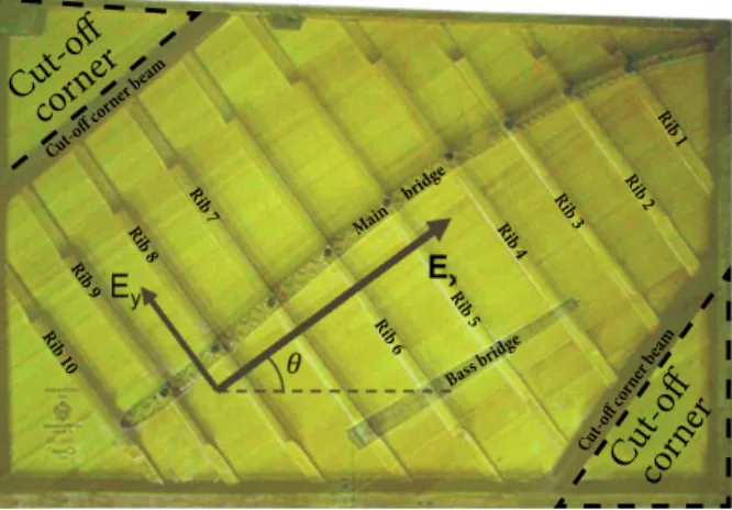
bridges almost parallel to the fibers, on the opposite side. Fig. 1 shows an example of 12

such a structure. 13

The vibro-acoustic broadband behavior of this structure has been studied by several 14

authors including Fletcher [2], Weinrech [3], and Kindel [4], then by Suzuki [5], [6], 15

Conklin [7]–[9], Giordano [10]–[12], Dérogis [13], Berthaut [14], Bensa [15], Stulov [16], 16

and more recently by Ege and Boutillon [17], [18], Chaigne [19], Chabassier [20], 17

Rigaud [21], and Etcheniquel [22]. It is now the subject of software development for 18

piano sound synthesis [23]. 19

Many other works already exist on the subject of ribbed structures and not only in the 20

area of musical instruments. Indeed, nowadays simple structures like beams and 21

isotropic plates are described well [24]–[33], but the design and modeling of ribbed 22

structures nonetheless remains a major topic of research. Most of these studies have 1

focused on periodically ribbed isotropic flat plates [34]–[44], curved panels [45], 2

stiffened cylindrical shells [46]–[53], and more recently laminated composite panels [54], 3

[55] and sandwich structures [56]–[59]. 4

Problems linked to the piano soundboard have been studied from the angle of purely 5

musical issues. These included the quest for a good compromise between “sustain / 6

radiated power” and poor color in high frequencies (i.e poor spectrum of last notes), 7

both of which appear to be the main difficulties confronting piano makers. 8

Although modelling flat ribbed structures and their baffled radiation has long been an 9

area of research, taking into account non-rectangular geometry, non-special orthotropy 10

(i.e. the axes of orthotropy are not parallel to the boundary if rectangular) and attached 11

bars in orthogonal directions simultaneously is a real challenge. 12

With a view to solving these issues, modelling is performed using a variational approach 13

in which the judicious use of simply supported rectangular extended plate modes and 14

radiation impedances is introduced. The aim of this model of an upright piano 15

soundboard, which avoids any object discretization, is to provide an interesting 16

alternative to a complete numerical method such as the FEM-BEM method (with long 17

computing time), which could obviously be used. 18

Consequently, this model facilitates parametrical studies and, for example, highlights 19

the influence of ribs and bridges (numbers, width, length, height) on the acoustical 20

radiation of the piano soundboard and, more generally, on orthotropic ribbed panels. 21

This article is the continuation of works presented in [60]. The first part of the article 1

presents how the non-rectangular edges and orientation of the materials composing the 2

piano soundboard are formulated by the addition of springs. Then, in the second part, 3

the model of the soundboard of a Pleyel P131 is described. It comprises the addition of 4

ten ribs, two bridges and two “cut-off” corner beams. The modal aspects are presented 5

in the frequency range 0; 3000 Hz. In particular we discuss the different families of 6

modes due to stiffening. Then, several numerical results including mobility and acoustic 7

radiated power are presented for an excitation moving along the main bridge at the 8

position of the string couplings. We show how the vibro-acoustical behavior of the 9

soundboard depends on the positions of the strings, and how the discrete frequencies 10

of the notes (the sources) make analysis difficult. 11

Drawing its inspiration from [61], [62], a parametrical study shows the complexity of 12

obtaining homogeneous high-pitched notes and how it is related to the soundboard 13

design (main bridge discontinuity, ribs in the high frequency domain, etc.). This is done 14

by introducing a new indicator applied to the mobility and the acoustic radiated power, 15

taking into account the discrete spacing aspects (discontinuous excitation points) and 16

the discrete frequencies of the keys at the same. 17

II. O

18

In traditional piano soundboard design, the direction of the wood fibers is not parallel to 19

the edges: we define this as the angle of orthotropy 𝜃. See Fig. 1. In this part we focus 20

on a method of modeling the orientation of the fibers and describing the non-rectangular 21

contours. We demonstrate the originality of this method which allows us to describe, 22

from the analytical standpoint, any shapes embedded within a rectangular shape, and to 1

take into account non-specified orthotropy, i.e. when the main axes of orthotropy are not 2

parallel to the soundboard shapes. 3

4

Fig. 1 - (Color online) Upright piano soundboard of Pleyel P131 with Ex and Ey being the strong and the

5

weak Young’s moduli of the wood. View from front side (bridge side) with ribs and cut-off corner

6

beams added in transparency.

7

II.A. T

8

In order to describe both the non-rectangular contours and the unspecified angle of 9

orthotropy, the following model uses the simple basis of a special rectangular 10

orthotropic plate, i.e. the Young’s moduli are parallel to the plate edges. See Fig. 2 on 11

the left. By adding several springs (dark points) to block the transverse displacement, 12

we describe the non-rectangular contours and the unspecified angle, as shown in 13

Fig. 2 on the right. The boundary conditions will tend to clamped conditions. 14 Cut-o ff corn er Cut-o ff corner Main b ridge Bass brid ge Cut-o ff corne r bea m Cut-off c orner be am Rib 1 Rib 2 Rib 3 Rib 4 Rib 5 Rib 6 Rib 7 Rib 8 Rib 9 Rib 10

1 Fig. 2 - (Color online) The addition of springs on a rectangular simply supported plate. On the left: the 2 initial plate with specific orthotropy; on the right: the addition of springs. The non–rectangular 3 contours and the non-specified angle of orthotropy are well described. 4

Thus it is possible to describe any edges the user wishes (not limited to only 5

soundboards) as suggested in Fig. 3. Obviously, it is possible to model a grand piano 6

but we chose to study a Pleyel P131 upright soundboard available at the lab (kindly 7

given by ITEMM, European Technological Institution for Music Professions). 8 9 Fig. 3 - (Color online) Examples of possible geometries with different orthotropy angles and edges. 10

II.A.1. H

The model is based on a variational approach. We express the Hamiltonian of the 12

whole plate-spring system to determine the eigenvalue problem (no external works 13 E_x E_y E_x E_y !! Lx Ly Lx Ly

are considered). An additional external force will be introduced in II.A.3 for the 1

forced response calculation. 2

The starting point of our modeling is a simply supported rectangular plate with 3

specific orthotropy. It follows the thin plate Love-Kirchhoff hypothesis for which the 4

Hamiltonian can be easily found in the literature [25]. Additional information on the 5

kinetic hypothesis can be found in a previous article [60]. 6

We consider several springs coupled to the plate at the coordinates 𝑥_&, 𝑦_& . We 7

give the following Hamiltonian for a plate with a number of springs Ns:

8 𝐻_*+= 1 2 𝜌ℎ𝑤˙ 3− (𝐷7𝑤,883 + 𝐷:𝑤,;;3 + 𝐷3𝑤,88𝑤,;;+ 𝐷<𝑤,8;3 ) >? ;@A >B 8@A 𝑑𝑥𝑑𝑦 DE DF 𝑑𝑡 + −1 2 𝑘𝑤3 𝑥, 𝑦 𝛿(𝑥 − 𝑥&)𝛿(𝑦 − 𝑦&) >? ;@A >B 8@A 𝑑𝑥𝑑𝑦 DE DF 𝑑𝑡 JK &@7 (1)

with 𝑤 being the plate transverse displacement; 𝑘 the spring rigidity; 𝑡_A; 𝑡₇ an 9

arbitrary time interval; 𝐿₈ and 𝐿_; the plate dimensions; 𝜌 the plate mass density; ℎ 10

the plate thickness; 𝐷₇ =_{ET EUVB?V?B}QBRS , 𝐷_: =_{ET EUVB?V?B}Q?RS , 𝐷₃ = _{W EUVB?V?B}V?BQBRS and 𝐷_< =XB?RS_S 11

the plate dynamic stiffness; 𝜈8; and 𝜈;8 = 𝜈8;𝐸; _𝐸8 its Poisson coefficients;

12

𝐸₈ and 𝐸_; the two Young moduli of the plate. 13

The first line of the equation is related to the plate and the second to the springs 14

where the Dirac distributions render them localized at the coordinates 𝑥&, 𝑦& .

15

Table 1 gives the properties of the extended rectangular orthotropic spruce plate 16

II.A.2. M

As mentioned previously, the starting point of our model is a rectangular simply 2

supported plate. This basis, currently used in the area of vibrations, is particularly 3

adapted for an analytical approach and has been studied several times [26], [46], 4

[63]. Of course, this basis is not the real basis of the embedded plate but only a 5

convenient basis for our model, as will be shown in the following. Using modal 6

decomposition, the transverse displacement is written as a linear combination of 7

simply supported plate modes weighted by modal amplitudes 𝑎_\] 𝑡 : 8 𝑤 𝑥, 𝑦, 𝑡 = 𝑎_\] 𝑡 𝜙_\] 𝑥, 𝑦 J ]@7 _ \@7 ∀𝑥 ∈ 0; 𝐿₈ and 𝑦 ∈ 0; 𝐿_; (2)

where 𝜙\] 𝑥, 𝑦 = sin 𝑚𝜋 𝐿₈𝑥 sin 𝑛𝜋 𝐿_;𝑦 .

9

By injecting the modal decomposition (2) into Eq. (1) and using the orthogonal 10

properties of eigenvectors, it is possible to analytically calculate the surface 11

integral in the Hamiltonian. Thus the functional depends on the two variables 12

𝑎_\] 𝑡 , 𝑎_\](𝑡) and no longer on the transverse displacement 𝑤 𝑥, 𝑦, 𝑡 and its 13

space and temporal derivatives. Thus we have: 14 𝐻_*+(𝑎_\](𝑡), 𝑎˙_\](𝑡)) = DEℒ DF (𝑎_\](𝑡), 𝑎˙_\](𝑡)𝑑𝑡 (3) where ℒ(𝑎\](𝑡), 𝑎 ˙

\](𝑡)) is termed the Lagrangian of the system.

15

By applying the differential form of the principle of least action and using 16

Euler-Lagrange equations, the action of the system is minimized, leading to the 17

following homogeneous linear system: 18

𝑀+ijDk_{+ 𝑀}&+lm]n& _{𝑎+ 𝐾}+ijDk_{+ 𝐾}&+lm]n& _{𝑎 = 0 (4)}

where 𝑀 and 𝐾 represent mass and rigidity matrices. These matrices are 1

constituted by the sum of diagonal matrices coming from the plate and full and 2

symmetrical matrices from the springs. 3

Solving the corresponding eigenvalue problem Eq. (4) allows calculating the 4

modes of the embedded plate: eigen-frequencies and modal shapes, the matrix of 5

eigenvectors and thus the transfer matrix 𝑇 between the initial simply supported 6

basis and the system basis, which is the orthonormed basis of the eigenvectors 7

[60]. We give the relation between the two bases with 𝑎 and 𝑏 being the vectors of 8

modal amplitudes in the initial basis and in the new basis, respectively: 9

𝑎 = 𝑇𝑏 (5)

Consequently, the real modal shapes of the embedded plate are built as a linear 10

combination of the simply supported shapes of the extended plate: 11 𝛷 m _{𝑥, 𝑦 = 𝑎} \] (m) _𝜙 \] 𝑥, 𝑦 J ]@7 _ \@7 ∀𝑥 ∈ 0; 𝐿₈ and 𝑦 ∈ 0; 𝐿_; (6) Where 𝑖 indicates the column number in the matrix of eigenvectors.

12

Note that the size of these matrices, which is governed by the truncation on the 13

orders M and N in the finite modal decomposition Eq. (2), determines the precision 14

of the results. 15

II.A.3. F

and harmonic external force applied at point (𝑥k, 𝑦k) with an amplitude of 1N.

1

Following the same approach as before, we determine the vector of generalized 2

force 𝐹nk] (second member of Eq. (4)) for which the components are defined by:

3

𝐹_+u= 𝜙_+u(𝑥_k, 𝑦_k) (7) To determine the forced response of the system we choose to express the 4

problem in the system basis. Using Eq. (5), the generalized matrix problem Eq. (4) 5

with the second member becomes diagonal: 6

−𝜔3_𝑀

*+𝑏(𝜔) + 𝑗𝜔𝐶𝑏(𝜔) + 𝐾*+𝑏(𝜔) = 𝑇D𝐹nk] (8)

With 𝑀*+ = 𝑇D 𝑀+ijDk+ 𝑀&+lm]n& 𝑇 and 𝐾*+ = 𝑇D 𝐾+ijDk+ 𝐾&+lm]n& 𝑇.

7

The modal damping matrix 𝐶 is also introduced. The structure is considered as a 8

weakly dissipative system for which the equations of generalized displacements 9

are uncoupled [64]–[66] so the matrix 𝐶 is also diagonal and defined by: 10

𝐶 = ⋱ 𝜂m𝑚m𝜔m

⋱

(9)

With 𝑚m, 𝜔m and 𝜂m being the modal mass, angular frequency and damping loss

11

factor of the ith system mode. 12

In the case of a piano soundboard, the modal loss factor was evaluated between 13

1% and 3%, depending on the modes in our frequency range of interest [67]. In the 14

following, the modal loss factors of all the soundboard modes are fixed at 2%. 15

II.B. S

Minimal spring rigidity and spacing are necessary to block transverse displacement. 2

For the frequency range of interest 0; 3000 Hz , the spacing between springs 3

depends on the smallest wavelength in the plate. The latter is in the direction of the 4

weak Young’s modulus [67]: 5 𝜆 = 2𝜋 𝑓 𝐷_: 𝜌ℎ 7/< (10)

A criterion of 𝜆 10 is chosen to overestimate the number of springs. In the present 6

case, it leads us to a minimal distance between the springs of around 7.3 mm (for f = 7

3 kHz). 8

Minimal spring rigidity is also important: the ratio between the rigidity of the spring 9

and that of the plate must be sufficiently high. When the rigidity is insufficient, 10

vibrations appear at high frequencies in the “blocked” area (where the springs are 11

localized). 12

We define the ratio between the average quadratic velocity in the free area and the 13

whole plate as a criterion in order to validate sufficient spring rigidity: 14 𝐿_{€ ratio} = 10 𝑙𝑜𝑔 𝑣(𝑥, 𝑦) 3 ˆ‰Š‰ 𝑑𝑆 𝑣(𝑥, 𝑦) 3 ˆŒ•‰ 𝑑𝑆 (11)

For a sufficient value of spring rigidity the velocity on the blocked area will tend to 15

Fig. 4-a presents this ratio for two spring rigidities. In both cases, the truncation order 1

is fixed at 𝑃, 𝑄 = (82,63) for which the convergence of the solution is guaranteed. 2

The excitation point is arbitrarily chosen near an edge. 3 4 Fig. 4 - (Color online) Influence of spring rigidity. 5 a) Average quadratic velocity ratio for two spring rigidities. Solid line: sufficient rigidity; dashed line: insufficient 6 rigidity. The excitation is placed at (xe,ye)=(1.26,0.76). 7 b) Modal density per octave for two spring rigidities and analytical plot from [11], [17], [67] Eq. (A.13): circle 8 markers: sufficient spring rigidity; square markers: insufficient spring rigidity; solid line: analytical expression. 9

When the springs are strong enough compared to the plate, the ratio is lower than 10

0.06 dB for the entire frequency range (solid line in Fig. 4-a). On the contrary, 11 102 103 0 0.5 1 1.5 2 2.5 3 3.5 Frequency [Hz] L v ratio = 10*log (<v to t > 2 /<v in t > 2 ) [dB]

Sufficient spring rigidity (k=2,5E6) Insufficient spring rigidity (k=2,5E4)

102 103 0 0.05 0.1 0.15 0.2 0.25 0.3 0.35 Frequency [Hz] n(f) [modes.Hz −1 ]

Analytical modal density of a clamped plate with an angle of orthotropy of −34.804 ° Sufficient spring rigidity (k=2.5E6) Insufficient spring rigidity (k=2.5E4)

a)

insufficient springs imply a higher velocity ratio (dashed line in Fig. 4-a) from 1 kHz 1

with a peak around 3.2 dB at 2.5 kHz in the present case. This lack of rigidity can 2

also be detected on the modal density (Fig. 4-b); see next paragraph. 3

Fig. 5 (on the left and center) presents modal shapes for these two cases. The modal 4

shapes are similar at low frequency. See top left and center of Fig. 5. Indeed, at low 5

frequency the ratios are equivalent. We can also note a small frequency difference. 6

From 1 kHz, three kinds of modes exist if the rigidity is insufficient: internal modes (in 7

the free area), external modes (in the density of springs) and hybrid modes (in the 8

two areas). The bottom left of Fig. 5 shows one of these undesired modes. On the 9

other hand, sufficient rigidity ensures only one kind of mode: the internal mode 10

(bottom center, Fig. 5). 11

As mentioned previously, the coexistence of these multi-type modes can also be 12

detected on the modal density. Fig. 4-b shows a comparison between the modal 13

density of the two cases of spring rigidity and the analytical formulation from [17], 14

[67]. This comparison shows good agreement of the modal density with the 15

theoretical plot (solid line in Fig. 4-b) when the rigidity is sufficient (circle markers in 16

Fig. 4-b) and tends toward the same value. On the contrary, when the spring rigidity 17

is insufficient, the presence of external modes implies a considerable increase of 18

modal density (square markers in Fig. 4-b). This effect is very interesting and 19

appears even if the order of truncation is not adapted. It can facilitate the detection of 20

external modes by solving only the eigenvalue problem. 21

1 Fig. 5 - (Color online) Modal shapes of a clamped non-rectangular plate with an angle of orthotropy of 2 34.8°. Left: insufficient spring rigidity; Center: sufficient spring rigidity; Right: FEM-NASTRAN with a 3 mesh of 5mm. 4

We also compared our modelling with a NASTRAN FEM model. This is a 2D model 5

with a non-rectangular clamped plate meshed with orthotropic PSHELL elements. 6

The size of the elements is around 5mm to ensure the convergence of the 7

calculations for the whole frequency range of interest [0;3000] Hz. 8

The comparison between our analytical model (Fig. 5, center) and numerical FEM 9

(Fig. 5, right) shows that our solution is relevant. Indeed, the clamped boundary 10

conditions, frequencies and modal shapes are well-described by our method: the 11

MAC criterion is 0.9997 and 0.948 for the modes presented in Fig. 5, respectively the 12

first modes around 30 Hz and another around 1.8 kHz. Concerning the frequencies 13

the difference is less than 4%, which is perfectly acceptable. 14

III. M

In the following, we focus on the upright piano soundboard of a Pleyel P131. This 2

soundboard is made of spruce stiffened on one face by ten ribs also made of spruce 3

placed in the direction of the weak Young’s modulus and on the other face by a bass 4

bridge and a main bridge (medium and high pitched notes), made of beech, placed in a 5

direction nearly parallel to the strong Young’s modulus (wood fibers). There are also two 6

“cut-off” corners delimited by two beams made of beech. See Fig. 1. 7

III.A. S

:

8

The model of the superstructures is an extension of the model presented in [60]. 9

Indeed, it now allows having linear superstructures of different lengths in addition to 10

different materials, widths, heights and offsets from the middle plane of the plate. Fig. 11

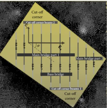
6 describes the geometry modeled. 12

1

Fig. 6 - (Color online) Geometry modelled for the Pleyel P131.

2

The model developed allows having only linear superstructures parallel to the entire 3

plate edges, i.e. in the direction of the wood fibers or perpendicular to them. Taking 4

into account a curved main bridge or a stiffener that is not parallel to an extended 5

plate edge will imply expressing variable 𝑥 as a function of 𝑦 and vice-versa. 6

Therefore it will be impossible to carry out simplifications useful for maintaining an 7

analytical approach as long as possible. Thus the bridges and “cut-off” corner beams 8

become exactly parallel to the strongest Young’s modulus Ex. The main bridge is cut

9

into two parts and shifted between ribs 3 and 4. Each has a constant height and 10

width. They are placed at position yc in the coordinates of the extended rectangular

11

plate. All the dimensions were measured on a real Pleyel P131 piano soundboard. 12

Table 2 gives the dimensions and properties of the superstructures. 13

The ribs are oriented perpendicular to the direction of the wood fibers and 14

perpendicular to the bridges to compensate for the weakness of the wood (weak 15 Rib 1 Rib 2 Rib 3 Rib 4 Rib 5 Rib 6 Rib 7 Rib 8 Rib 9 Rib 10

Cut-off corner beams 2

Cut-off corner beams 1

Cut-off corner

Cut-off corner Bass bridge Main bridge part 1

Young’s modulus Ey). Thus the ribs have a predominantly static effect. Their heights

1

are not constant along their lengths. Indeed, they are tapered at their extremities to 2

obtain flexibility near the edges of the soundboard. See Fig. 7-a. 3 4 Fig. 7 - (Color online) Rib geometry. a) Section view of a real soundboard rib. b) Simplified rib in the 5 present model. c) Partial front view of the soundboard. 6

In our model, this progressive decrease of height is simplified. We consider a sudden 7

change of the height, as shown in Fig. 7-b. All the ribs have a height of 5mm at their 8

extremities. Table 3 gives the dimensions and properties of the ribs. 9

The boundary conditions are applied to the middle plane of the plate. The ribs and 10

bridges are bound to it through a double continuity in displacement and rotation at 11

each interface. Moreover, their heights are sufficiently low to neglect the warping 12

phenomenon. Consequently, the plate controls the global motion of the whole system 13

and its motion field can be extended to the superstructures. In addition to the 14

continuity at the interface, the motion fields in the plate / stiffener sections are 15

considered linear [60]. We also take into account bending and torsion phenomena. 16

This leads us to express the Hamiltonians of each superstructure (for more 17 (c) (b) (a) ) ) )

𝐻_lm’ = 1 2 DE DF 𝜌_l 𝐼_”𝑤˙_,;3 _{+ 𝑏𝐻𝑤}˙ 3 _{− 𝐸} l𝐼”𝑤,;;3 + [𝜌l𝐼n𝑤,83 ;–@;Œ—>T ;@;Œ >B 8@A − 𝐺_l𝐼_n𝑤_,8;3 _{] 𝛿(𝑥 − 𝑥} l) 𝑑𝑥𝑑𝑦𝑑𝑡 (12) 𝐻_’lmšnk = 1 2 DE DF 𝜌_› 𝐼_”›𝑤˙_,83 _{+ 𝑏} ›𝐻›𝑤˙ 3 . −𝐸›𝐼”›𝑤,883 + [𝜌›𝐼n›𝑤,;3 >? ;@A 8–@8Œ—> 8@8Œ − 𝐺_›𝐼_n›𝑤_,8;3 _{] 𝛿(𝑦 − 𝑦} ›) 𝑑𝑥𝑑𝑦𝑑𝑡 (13)

Table 4 summarizes all the constants used in the previous equations. As in Eq. (1), 1

the entire Hamiltonian for the whole system (with Nr being the number of ribs and

2

extremities and Nb the number of bridges, for which all the constants and positions

3

are different) becomes: 4 𝐻_{&*•]š’*jlš} = 𝐻_*+ + 𝐻_lm’(l) Jž l@7 + 𝐻_’lmšnk(’) JŸ ’@7 (14)

and the eigenvalue matrix problem as described in section II.A.2: 5

𝑀𝑝𝑙𝑎𝑡𝑒+ 𝑀𝑠𝑝𝑟𝑖𝑛𝑔𝑠+𝑀lm’&_{+ 𝑀}’lmšnk& _{𝑎 + 𝐾}𝑝𝑙𝑎𝑡𝑒_{+ 𝐾}𝑠𝑝𝑟𝑖𝑛𝑔𝑠_{+ 𝐾}lm’&_{+ 𝐾}’lmšnk& _{𝑎 = 0 (15)}

Therefore we determine the new transfer matrix 𝑇 of the Pleyel P131 and the 6

generalized matrix formulation with a second member on the basis of the piano 7

modes: 8

−𝜔3_𝑀

With 𝑀_{&*•]š’*jlš} = 𝑇D 𝑀+ijDk+ 𝑀&+lm]n&+𝑀𝑟𝑖𝑏𝑠 + 𝑀𝑏𝑟𝑖𝑑𝑔𝑒𝑠 𝑇 and 𝐾_{&*•]š’*jlš} = 1

𝑇D _𝐾+ijDk_{+ 𝐾}&+lm]n&_{+ 𝐾}𝑟𝑖𝑏𝑠_{+ 𝐾}𝑏𝑟𝑖𝑑𝑔𝑒𝑠 _{𝑇 . Damping matrix 𝐶 is the same as that}

2

presented in Sec. II.A.3. 3

III.B. A

-

4

The method we propose for acoustic radiation is an alternative to a purely numerical 5

method such as the finite element boundary method, Rayleigh integral or Perfectly 6

Matched Layers. Thus we calculate the acoustic radiation of the structure using the 7

radiation impedances of the extended rectangular un-ribbed plate, which has been 8

studied several times by Wallace, Maidanik and Stepanishen [34], [31], [30], for 9

example. This approach is currently limited to a rectangular ribbed plate [63] but we 10

propose to extend it to the case of a non-rectangular structure. In addition, this 11

approach allows comparing the radiation modal impedances of a non-rectangular 12

ribbed structure to those of an equivalent simple plate, as was done in our previous 13

article [60]. This could be particularly interesting in the frequency range where the 14

modes are similar to un-ribbed plate modes (i.e. at low frequencies). 15

We can consider that the piano case is an obstacle to acoustic short circuiting past 16

the first modes. At low frequency, this results in a decrease of radiation [26], [32]. On 17

the contrary, when focusing on frequencies higher than the first octave, as will be the 18

case in the following, the wavelengths quickly become small enough to consider a 19

baffled hypothesis. Note that this hypothesis does not change the tendencies of the 20

The light fluid assumption is also made as it implies omitting inter-modal coupling 1

brought by the action of a fluid on the structure. Several authors have shown that 2

these couplings are negligible at the first order [31], [68], [29] or do not change the 3

general tendencies [69], [41], [54]. However, other authors have shown that some 4

changes can occur in the case of heterogeneous boundary conditions, high 5

superstructures or at resonances [70], [71]. We assume that they are neglected and 6

thus assign the acoustic radiated power 𝑊 𝜔 of the piano soundboard in the 7 frequency domain as [60], [29]: 8 𝑊 𝜔 =𝜔3 2 𝑏 D ∗𝑇D𝑅(𝜔)𝑇𝑏 (17)

with 𝑅 𝜔 being the real part of the inter-modal acoustical impedance matrix. 9

Due to the light fluid assumption this matrix is diagonal, i.e. inter-modal couplings are 10

neglected. Thus the diagonal terms are calculated numerically and defined as [26], 11 [29]: 12 𝑅\]\](𝜔) = 𝜌_A𝜔 𝜋3 |𝜙_\](𝑘₈, 𝑘_;)|3 𝑘3_{− 𝑘} 83− 𝑘;3 ¨ A 𝑑𝑘8𝑑𝑘; (18)

where 𝜙\](𝑘8, 𝑘;) refers to the bi-dimensional Fourier transform of a simply

13

supported rectangular baffled plate mode. 14

III.C. N

P

P131

15

The vibro-acoustical behavior of the piano soundboard can be split into different 16

frequency ranges in which the vibration and radiation are different, due to the design 17

of the instrument. In the following, we will first focus on the modal aspects of the 1

instrument and then on the vibro-acoustical response of the soundboard. 2

To ensure the convergence of the calculations, the truncation order on the modal 3

basis is overestimated and, as with the unribbed plate, fixed at (M,N)=(82,63). 4

Moreover in order to validate the blocking condition along the non-rectangular 5

contours, the same studies as shown in Figs 4 and 5 were performed (spring rigidity 6

and number). 7

III.C.1. S

8

In terms of modal shapes, many phenomena appear as a function of the frequency 9

range considered. Indeed, the more the frequency increases, the higher the rigidity 10

of the superstructures is. Therefore the superstructures will strongly limit the 11

transverse displacement of the soundboard when the frequency increases. This 12

begins with the strongest of superstructures, i.e. the bridges, and then the ribs. 13

Some studies have also shown that the vibration is localized in certain frequency 14

ranges. Waveguide effects occur when the wavelengths reach the same order of 15

magnitude as the inter-rib spaces [17], [18]. Fig. 8 shows a classification of modal 16

shapes for the 200 first modes (below 3 kHz). We define four families of modes: 17

• “Similar” to plate modes, i.e. unribbed modes that can be named with the 18

number of half wavelengths in the different directions (mode (3,1) for 19

example); 20

• Blocking bridges and ribs, when all the superstructures strongly minimize 1

the plate transverse displacement; 2

• Localized vibrations, when the vibration is localized in a small area 3

delimited by the superstructures. 4

5

Fig. 8 - (Color online) Classification of the first 200 modes of a Pleyel P131 soundboard.

6

To classify the modal shapes into these different families, we use an average 7

quadratic linear velocity to evaluate numerically when the vibration is reduced at 8

the stiffener locations. This allows determining the points at which the transverse 9

displacement is strongly limited. To do this, we define a velocity threshold that 10

allows separating a sample of modes classified visually previously (around 20 11

modes). Regarding the “localized vibrations” family, which is a sub-family of 12

“blocking bridges and ribs”, a criterion of spatial distribution is added. We first 13

detect the maximum velocity magnitude of the structure and then compare the 14

entire space average quadratic velocity with the space average quadratic velocity 15

1 21 41 61 81 101 121 141 161 181 201

"Similar" to plate modes Blocking bridges only Blocking bridges and ribs Localized vibrations Mode number Mode famillies 99 816 1228 1575 1845 2090 2297 2490 2688 2875 3094 3% 4% 66% 24% = 10% + 14% Frequency [Hz] Classified modes: 96% 99 816 1228 1575 1845 2090 2297 2490 2688 2875 3094 3% 4% 66% 24% = 10% + 14% 99 816 1228 1575 1845 2090 2297 2490 2688 2875 3094 3% 4% 66% 24% = 10% + 14% 99 816 1228 1575 1845 2090 2297 2490 2688 2875 3094 3% 4% 66% 24% = 10% + 14%

Into "cut−off" Corners Out of "cut−off" Corners

Localized vibrations Blocking bridges and ribs Blocking bridges only «Similar» to plate modes 24% = 10% + 14% 66% 4% 3%

on a smaller surface around the maximum magnitude determined previously. We 1

gradually increase the surface so that the local average velocity becomes higher 2

than a certain percentage of the entire space average velocity. Similarly, this 3

percentage is determined with a sample of modal shapes classified visually. In this 4

way, we can classify around 73% of the modal shapes that are checked visually as 5

a final control. The unclassified modes are determined visually and we finally 6

classify 96% of the modes into the four families. 7

We can see that the ratios between them are very different. Indeed, for a large 8

majority of modes all the superstructures strongly minimize the transverse 9

displacement (sum of triangle markers around 90%), whereas the modes “blind” to 10

the superstructures amount to only around 3% (see the square markers on Fig. 8). 11

They match with low frequencies when the wavelengths are high compared to the 12

dimensions of the soundboard. Fig. 9 shows two examples of these low frequency 13

modes, with one of them similar to mode (1,1) and the second similar to mode 14

(3,1). This phenomenon is limited to the five first modes of the soundboard. 15

16

Fig. 9 - (Color online) Low frequency modes similar to unribbed plate modes.

17

A second family can be associated with the frequency range 300; 900 Hz when 18

displacement of the plate. This family is illustrated in Fig. 10 and matches with the 1

circle markers in Fig. 8. 2 3 Fig. 10 - (Color online) Modes where the transverse displacement is strongly minimized by the 4 bridges. 5

For the majority of modes (higher than 1 kHz), all the superstructures strongly 6

minimize the transverse displacement. For around 66% of them, the vibrations are 7

spread over the whole plate or at least over a large area (see the triangle markers 8

pointing to the right in Fig. 8). Fig. 11 shows two of these modes, the first around 1 9

kHz and the second around 3 kHz: the location of the superstructures can be 10 easily guessed. 11 12 Fig. 11 - (Color online) Modes where the transverse displacement is strongly minimized by all the 13 superstructures. 14

In addition, the vibrations are also localized in areas delimited by superstructures 15

for the last 24%. It is important to split these 24% into two sub-parts: 10% of “cut-16

off” corner modes (upward triangle markers in Fig. 8) and 14% of vibrations 17

401,9 Hz 790,3 Hz

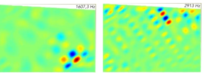
localized between the ribs (downwards triangle markers in Fig. 8). Fig. 12 shows 1

two examples of this 14% of modes. 2 3 Fig. 12 - (Color online) Modes where the vibrations are localized into areas delimited by 4 superstructures. 5

This phenomenon of localization between the ribs seems to begin at around 1600 6

Hz, thus when the wavelengths are around the same order of magnitude as the 7

inter-rib spaces [17], [18]. But as shown in Fig. 12, the percentage of this family is 8

quiet low compared to the “blocked modes” (only 14% vs. 67%): the wavelength 9

condition seems to be a necessary but not sufficient to localize the vibrations in a 10

reduced area of the soundboard. 11

Finally, the last 4% are unclassified modes: the bridges begin to minimize the 12

transverse displacement but not completely. 13

III.C.2. M

,

14

ACOUSTIC RADIATED POWER ALONG THE BRIDGE 15

The mechanical mobility at the bridge is an essential quantity in musical acoustics 16

because it characterizes the transfer between the source and the radiator. Several 17

piano soundboard studies exist on the subject [11], [18]. In the case of a harp 18

2913 Hz 1607,3 Hz

the excitation correspond to the coupling points between the soundboard and the 1

strings) as function of the frequency have been performed by [61], [62]. 2

However, the utility of mobility is limited to the local vibration at the excitation point. 3

In addition, we think it is worthwhile completing the analysis with other indicators, 4

such as space average quadratic velocity and acoustic radiated power, which take 5

into account the entire vibration of the soundboard. In this way, we consider an 6

excitation located on different points of the main bridge, corresponding to the string 7

coupling points ranging from note 32 (E3 with a fundamental frequencyof f0=164.8

8

Hz) to 76 (C7 with f0=2093 Hz), so from the left to the right of the entire main

9

bridge (parts 1 and 2) in Fig. 6. 10

Fig. 13 shows, from top to bottom: the mobility, the space average quadratic 11

velocity and the acoustic radiated power. Each of them is expressed in dB scale, 12

plotted with the same dynamic of 60 dB. 13

Note that in the case of a harmonic problem when considering the modal 14

decomposition Eq. (2) and the relation between the initial and piano basis Eq. (5), 15

the space average quadratic velocity in the soundboard area is given by the 16 following expression [29]: 17 𝑣3_{(𝜔) =} 𝐿8𝐿; 𝑆_m]D 𝜔3 8 𝑎\] 𝜔 3 J ]@7 _ \@7 = 𝐿8𝐿; 𝑆_m]D 𝜔3 8 𝑏 D ∗(𝜔)𝑇D𝑇𝑏(𝜔) (19)

where t refers to the transpose matrix or vector and * to the complex conjugate. Sint

18

is the surface of the soundboard, i.e. the unblocked surface. Regarding the 19

radiated acoustic power, its expression was given in Eq. (17). 20

1 Fig. 13 - (Color online) Evolution of local and general indicators at string/main bridge coupling points: 2 Top: mobility; Center: space average quadratic velocity; Bottom: Acoustic radiated power. 3

Globally, the three indicators follow the same trends. Firstly, dB levels tend to 4

decrease when the frequency increases. Moreover, the strings coupled near the 5

extremity and near the cut-off of the main bridge are sensitive to the local and 6

sudden change of the bridge height. Thus, there is an increase of mobility, space 7

average quadratic velocity and acoustic radiated power around 0.3 m and 1.2 m in 8

Fig. 13, i.e. near the beginning of the bridge and near its break. 9

Secondly, in the frequency range [400;3000] Hz the dynamic level is around 1/3 10

lower than 400 Hz. This becomes more apparent at high frequency when the 11

modal overlap masks the mode resonances. 12

However, the dynamic level of the mobility is higher than the others, regardless of 1

the frequency range (see Fig. 13). This is consistent because mobility is a local 2

indicator whereas the others take into account the entire behavior of the 3

soundboard. Below 400 Hz, the mobility fluctuates around 65 dB whereas the 4

space average quadratic velocity and the radiated power only around 40 dB, so 5

around 1/3 lower. Above 400 Hz, the ratio is around the same order of magnitude. 6

III.C.3. M

7

VIEWPOINT 8

From the musical viewpoint, the large quantity of information in this kind of 9

presentation makes it difficult to interpret the results. Indeed, the response of an 10

instrument is not continuous in frequency but discrete, in addition to the discrete 11

variation of the excitation position. In the case of a harp soundboard, [61], [62] 12

focused on admittance at discrete frequencies corresponding to string 13

fundamentals. These authors also did the same for the first and the second 14

partials, neglecting the inharmonicity brought about by mobility, i.e. by simply 15

multiplying the fundamental frequencies. In the following, we extend this idea to 16

the acoustic radiated power. This study is limited to partials due to string 17

transverse waves below 3 kHz. We present the average values of each indicator 18

and the gradients between successive notes (in absolute values) from the 32th to 19

76th. All the partials have the same magnitudes. We give the following expressions 20

for the average values of mobility and acoustic radiated power: 21

𝐿_ 𝑘𝑒𝑦 = 20 𝑙𝑜𝑔 1 𝑁_+jlDmji& 𝑤(𝑥¨k;, 𝑦¨k;, 𝑛 𝑓¨k;) 𝐹 J«¬ž‰Œ¬-K ]@7 (20) 𝐿_® 𝑘𝑒𝑦 = 10 𝑙𝑜𝑔 1 𝑁+jlDmji& 𝑊(𝑥_¨k;, 𝑦_¨k;, 𝑛 𝑓_¨k;) 𝑊lk” J«¬ž‰Œ¬-K ]@7 (21)

Obviously, we are still far from a realistic force because the different partials do not 1

have the same amplitudes in reality. However, the advantage of these indicators is 2

that they present “pictures” of pianos, making it possible to compare different 3

instrument designs. 4

In all the following figures, the X-axis limits are the same but the labels are 5

different. That of the radiated power corresponds to the note numbers with the 6

related note names whereas that of the mobility corresponds to the fundamental 7

frequencies of each note. Moreover, all these figures are plotted with the same 8

dynamic in order to compare the variation of each indicator. 9

1 Fig. 14 - (Color online) Evolution of mobility (top) and acoustic radiated power (bottom) of a P131 2 soundboard. Left: dB values of indicators; Right: gradients (absolute values) between two successive 3 notes in dB. 4

Up to now, we have only focused on the results relating to the P131 soundboard 5

(Fig. 14). A major tendency is the inhomogeneity of mobility and power levels 6

along the bridge (left Fig. 14), particularly at the bridge break between notes 58 7

and 59, where both increase considerably. The same applies for the notes near 8

the beginning of the main bridge (near notes 32) where dB levels have the same 9

orders of magnitude as at the break. 10

The inhomogeneity of the response along the bridge is not limited to its beginning 11

and break. Regardless of the indicators, focusing on discrete frequencies also 12

shows that the higher variations appear after the bridge break, which is not 13

obvious on the mobility map view in Fig. 13. Above note 59, the wavelengths 14

become small and the waves no longer pass through the bridge break, contrary to 15

waves with lower frequencies. Therefore the second part of the main bridge 16 Rib 1 Rib 2 Rib 3 Rib 4 Rib 5 Rib 6 Rib 7 Rib 8 Rib 9

(almost half the size of the first part of the main bridge, see Fig. 6) cannot 1

distribute the vibration over the whole soundboard. 2

Moreover, the latter notes suffer from poor harmonic richness that maximizes the 3

variations. Indeed, in the case of the first notes, the large number of harmonics will 4

average the soundboard response, partly masking this phenomenon. Thus our 5

model shows that the higher the order of notes is, the greater the variability may 6

be. 7

This raises the question of the “killer-octave” which is, according to piano makers, 8

around the penultimate octave (C6 to C7). Fandrich [72] describes it as a region in 9

the fifth to sixth octave (C5 to C6) of the keyboard. In both cases, it is 10

characterized by low sustain and is present in most pianos regardless of 11

construction method or soundboard design. Our results show two areas that could 12

correspond to this phenomenon: the first with a large increase of the mobility and 13

the acoustic radiated power; the second their decrease. 14

Focusing only on the average values would lead to an incomplete study. Indeed, in 15

a playing situation, a major variation between two consecutive notes implies 16

considerable perceptive inhomogeneity for the pianist and the listener. With this in 17

mind, the gradients between successive notes provide much interesting 18

information (right, Fig. 14). They show considerable variability between two 19

successive notes and thus heterogeneous playing: the average mobility and 20

acoustic radiated power gradients are around 1.33 and 1.23 dB, respectively. 21

The soundboard response can also be split into two ranges of notes. For the third 1

and fourth octaves, the note-to-note gradients are low and the responses are 2

globally homogeneous, which is also the case for both the mobility and the 3

acoustic radiated power. Above the beginning of the fifth octave at around 659 Hz, 4

the gradients increase, with higher values of around 4 dB. Thus, for high-pitched 5

notes, it is common to have a perceived acoustic power division or multiplication 6

by 2.5 compared to the previous notes. The same effect occurs near the beginning 7

of the bridge but to a lesser extent. Note that a significant mobility gradient does 8

not systematically mean the same for the acoustic radiated power and vice-versa. 9

Moreover, we do not find a regular relationship between a decrease of the 10

indicators and the location of the ribs (represented by dashed lines in Fig. 14): 11

sometimes a coupling close to a rib tends to decrease the three indicators and 12

sometimes it tends to increase them. 13

To review, the behavior can be split into two main ranges: after the bridge break, 14

where the note–to-note gradients are higher and where there are major global 15

variations of mobility and acoustic radiated power; before the bridge break where 16

global variations of mobility and radiated power also exist but are lower. High-17

pitched notes (and the first notes) seem to be particularly difficult to control by 18

piano makers, contrary to medium notes. 19

Applying a force at the bridge tends to distribute the force over the entire plate and 20

thus homogenize the piano soundboard response. In the case of discontinuities, 21

this distribution effect is broken if the discontinuity is significant enough compared 22

to the wavelength of the wave propagated: at low frequencies, the wavelengths 1

are long and the discontinuity has no impact on the propagation; at high 2

frequencies, the wavelengths are short and a discontinuity will be an obstacle to 3

the propagation of waves. 4

Finally, as with all string instruments, piano strings have multiple modal 5

frequencies called partials or harmonics. For 32th note, there are 18 frequencies 6

below 3 kHz, whereas there is only one for the last note studied, number 76. Thus 7

a discontinuity could have a higher influence on high-pitched notes and on the high 8

order harmonics of the first notes. Consequently, it seems that if a bridge break is 9

necessary in the design of the instrument it could be placed at low frequency to 10

minimize its effect. On the contrary, the removal of any break at the bridge would 11

homogenize the response of the instrument. 12

III.D. E

13

To confirm the hypothesis made in our model, some comparisons were made with 14

the Nastran FEM method and experimental results. The measurements were 15

performed in the framework of an internship Master degree [73]. We present several 16

results in this paper to validate the hypothesis made in our model. The Pleyel P131 17

soundboard used was separated from the case and clamped to a solid wall made of 18

concrete to recreate baffled conditions. The structure was excited at the bridge in the 19

treble zone with a white noise and the vibration measured on the rib side with a 20

agreement between the modal shapes and those of our model, as shown by the 1

images in the top row in Fig. 15, for low frequency modes. In addition, the lower 2

images in Fig. 15 give examples of high order modes around 2 kHz, where the 3

superstructures strongly minimize the vibrations. 4 5 Fig. 15 - (Color online) Comparison of Pleyel P131 modal shapes between our analytical modelling 6 and experimental results. 7

However the first eigen-frequencies were higher in our model: the experimental 8

eigen-frequency was around 66 Hz whereas that of the analytical model was around 9

100 Hz. Therefore the acoustic radiation was overestimated around the first modes 10

without, however, changing the general trends. These differences highlight that the 11

structure in our model was too rigid. This was not due to geometrical simplifications 12

(superstructures parallel to plate edges, rib heights, etc.) since the spatial aspects 13

(modal shapes) were well-described and compared with the measurements. 14

Experimental results Analytical modelling

However, membrane effects may have had an impact on the eigen-frequencies of the 1

first modes and quickly disappeared. To determine whether this was the case, we 2

compared the experimental and our own results with a Nastran FEM model with the 3

same geometrical simplifications. In order to confirm the geometrical simplifications, 4

they were also simulated in the FEM model. The plate was meshed with PSHELL 5

elements and the superstructures with PBEAM elements deported on each face. The 6

FEM model is shown in Fig. 16 in which we consider two cases: the first with a 7

blocked membrane imposing no displacements of the plate elements; the second 8

with a membrane effect. 9 10 Fig. 16 - (Color online) Nastran FEM model of Pleyel P131 soundboard with the same geometrical 11 simplifications as in our model. a) and c) view of ribs view with cut-off corner beams; b) and d) bridge 12 view. 13

To ensure the convergence of the calculations, the size of the finite elements must be 14

a) b)

if it slightly increases the precision of our calculations. This result also shows that 1

both models converge to the same solution via two different paths: our model 2

converged from the top (increasing the order of truncation provides flexibility) 3

whereas the FEM model converged from the bottom. 4 5 Fig. 17 - (Color online) Eigen-frequency convergences for our model and the Nastran FEM model 6 (without membrane) as a function of truncation order and the mesh size. 7

The comparison of the three modelling and experimental results shows that the 8

modal shapes are very similar, as shown in Fig. 18. This main result confirms the 9

geometrical simplifications made in our model. On the contrary, the frequencies are 10

different and also confirm our hypothesis relating to the membrane effect. Indeed, the 11

frequencies of the FEM model without membrane were close to the frequencies of 12

our model, whereas those of the FEM with membrane were close the experimental 13

frequencies. 14

These comparisons show that the geometrical simplifications were relevant. 15

Membrane effects have an influence on the first eigen-frequencies and thus imply an 16

overestimation of the acoustic radiation at low frequencies. However, it is important to 17

keep in mind that the aim of this model is to perform parametrical studies. Therefore, 18

even if the first frequencies were higher than those of the real soundboard, the 19 0 50 100 150 200 250 300 0 500 1000 1500 2000 2500 3000 3500 Frequency [Hz] Mode number Analytical modelling (P,Q) = (82,63) Analytical modelling (P,Q) = (120,100) MSC NASTRAN 5mm MSC NASTRAN 1mm

membrane effects do not change the conclusions resulting from the comparison 1

made with our model. 2 3 Fig. 18 - (Color online) Comparison of numerical and experimental modal shapes using four methods. 4 From left to right: analytical modelling, Nastran FEM without membrane, Nastran FEM with 5 membrane and experimental results. 6

Analytical modelling FEM Nastran without membrane FEM Nastrant with membrane Experimental results

f = 95,6 Hz f = 142,9 Hz f = 212,2 Hz f = 234,5 Hz f = 273,7 Hz f = 98,6 Hz f = 152,11 Hz f = 221,6 Hz f = 243,3 Hz f = 281,7 Hz f = 70,9 Hz f = 107,6 Hz f = 159,3 Hz f = 162,2 Hz f = 193,6 Hz f = 66 Hz f = 102 Hz f = 138 Hz f = 154 Hz f = 184 Hz

ensure the contact between the strings and the bridges. Applying and tuning the 1

strings have two consequences: the initial crown lowers and compression stresses 2

are applied to the plate edges. This phenomenon is known as “downbearing” and 3

implies an increase of the first eigen-frequencies, as was shown in [74] and [67] 4

where we can find crossed comparisons of [4], [8], [74]–[77]. 5

However, simple reasoning leads to conclusions to the contrary. Indeed, lowering the 6

crown implies decreasing the eigen-frequencies [78]. The same effect occurs when 7

compression stresses are applied to the plate [79], [64]–[66]. In both cases, it quickly 8

becomes negligible when the frequency increases. To explain this, it seems that the 9

initial crown produced by manufacturing implies a non-linear evolution of the first 10

eigen-frequencies of the soundboard. Thus the latter can increase or decrease 11

depending on the initial crown: the consequences depend on the soundboard [80]. 12

Nevertheless, neglecting downbearing effects does hinder parametrical studies in the 13

same as membrane effects: the frequency shift will be around the same order of 14

magnitude in all the following studies. 15

IV. S

16

From subsection III.C.3, we know that structural heterogeneities imply variations of the 17

piano soundboard response, probably leading to a discontinuous timbre or perceived 18

sound, which is a difficulty expressed by piano makers. Although the components of the 19

force injected at the coupling point with the bridge do not have the same magnitudes, 20

we think that ensuring a linear or progressive evolution of each indicator presented in 21

III.C.3 will be interesting from the musical viewpoint. At least, their variations and 22

especially the gradients should be greatly reduced in order to obtain more 1

homogeneous playing. 2

Therefore we wanted to see how the vibro-acoustic behavior is modified through 3

structural changes. Hence we now consider two additional cases illustrated in Fig. 19: 4

Pleyel P131 soundboard with a continuous main bridge; P131 soundboard with ribs 1 5

and 2 removed. These cases are compared to the reference case presented previously 6

in III.C.3. In order to simplify the reading, solid lines are used instead of markers 7

although we continue to focus on a spectrum of discrete frequencies. 8 9 Fig. 19 - (Color online) Different sets of upright piano soundboards based on the Pleyel P131 10 configuration. a) Reference case: Pleyel P131; b) Continuous main bridge; c) Removal of ribs for high-11 pitched notes. 12

IV.A. C

13

Obviously, a continuous main bridge implies eliminating the defect between note 14

numbers 58 and 59 because there is no longer any abrupt and local change of 15

stiffness (Fig. 20, left). Moreover, the waves are better spread all over the 16

Thus the global variations above note 56 are now lower than in the reference case 1

(left Fig. 14), regardless of the indicators. 2 3 Fig. 20 - (Color online) Comparison between the P131 soundboard analyzed in III.C.3 and the P131 4 soundboard with a continuous main bridge. 5

Concerning the note-to-note gradients, their average values are lower than in the 6

reference case, especially that of mobility (see average values in Fig. 20, right). 7

However, we can see that the gradients of high-pitched notes are lower but still 8

remain high for both indicators. In the case of the acoustic radiated power, it leads to 9

a perceived division or multiplication of this power by two from the previous notes (3 10

dB). For the notes originally placed before the bridge break, few changes can be 11

noted on the mobility gradients. On the contrary, a continuous bridge increases the 12

acoustic radiated power gradients in the frequency band [165;650] Hz. Therefore, as 13

the average radiated power gradients are around the same order of magnitude for 14

both cases, it appears that it is to the detriment of mid-frequency notes (fundamental 15 165 Hz 330 Hz 659 Hz 1319 Hz 2637 Hz −80 −75 −70 −65 −60

−55 Average values with all the partials below 3 kHz [dB]

LM = 20 log (Mz P1 3 1 )

P131 / Reference case P131 with a continuous main bridge

165 Hz −> 175 Hz−5 330 Hz −> 349 Hz 659 Hz −> 698 Hz 1319 Hz −> 1397 Hz 2637 Hz −> 2794 Hz 0

5 10 15

20 Gradients between two successive notes [dB] 1.33 1.06

Average values of mobility gradients

32 / E3 44 / E4 56 / E5 68 / E6 80 / E7 65 70 75 80 85 90 LW = 10 log (W P1 3 1 /W ref ) 32 / E3 −> 33 / F3−5 44 / E4 −> 45 / F4 56 / E5 −> 57 / F5 68 : E6 −> 69 / F6 80 / E7 −> 81 / F7 0 5 10 15 20 1.23 1.19 Average values of acoustic radiated power gradients

frequency lower than 650 Hz) and to the advantage of notes with a fundamental 1

frequency higher than 650 Hz. 2

IV.B. R

3

Contrary to the previous case, the removal of two ribs has no effect on the first part of 4

the main bridge (below note number 56 in Fig. 21). In this range, the changes are 5

negligible for both indicators, as much for the average values as for the gradients. 6

Obviously, the effect of the main bridge break remains, with a pronounced increase 7

of the two indicators around note number 58 (Fig. 21, left), and also significant local 8

gradients (Fig. 21, right). For high-pitched notes, the two indicators do not follow the 9

same trends, contrary to the previous cases. For high-pitched notes, the mobility 10

level increases because the stiffness becomes lower locally due to the removal of the 11

stiffeners (top left Fig. 21). The loss of mobility from notes 62 to 67 in the reference 12

case (900 to 1250 Hz) has now been eliminated. At higher frequencies, mobility 13

increases until note number 71 (1550 Hz) and finally decreases. Thus the removal of 14

ribs will lead to a lower sustain due to the quicker injection of string energies in high-15

pitched notes. 16

However, this solution presents the advantage of substantially decreasing the 17

gradient between notes: globally the ratio of average gradients is around 3/4 between 18

the two cases (Fig. 21, top right). Focusing above note number 62, this ratio falls to 19

around 1/2 with average gradients of 1.5 dB and 0.8 dB, respectively, for the 20

1 Fig. 21 - (Color online) Comparison between the P131 soundboard analyzed in III.C.3 and the P131 2 soundboard with ribs 1 and 2 removed. 3

As for the mobility, the acoustic radiated power is impacted after the bridge break and 4

seems to approximately follow a decreasing linear tendency, passing in the middle of 5

the reference case (Fig. 21, bottom right). However, some variations of radiated 6

power moving to high frequency remain. Consequently, the maximum gradient is only 7

slightly lower but its average gradient is the same. 8

Finally, for the high-pitched notes, removing the ribs implies higher mobility and thus 9

a lower sustain. By way of compensation, the variations of the two indicators are 10

lower than in the reference case. From the musical viewpoint, removing the ribs 11

allows more homogeneous playing with lower variations between consecutive notes 12

for this frequency range. 13

These parametrical studies show the difficulty of controlling the piano soundboard 14

response, particularly in the treble zone, which can be considered as a sensitive 15

range. For these notes, a structural change has a considerable effect on their 16 165 Hz 330 Hz 659 Hz 1319 Hz 2637 Hz −80 −75 −70 −65 −60 −55

Average values with all the partials below 3 kHz [dB]

LM = 20 log (Mz P1 3 1 )

P131 / Reference case P131 with two removed ribs

165 Hz −> 175 Hz−5 330 Hz −> 349 Hz 659 Hz −> 698 Hz 1319 Hz −> 1397 Hz 2637 Hz −> 2794 Hz 0 5 10 15 20

Gradients between two successive notes [dB]

1.33 1.01 Average values of mobility gradients

32 / E3 44 / E4 56 / E5 68 / E6 80 / E7 65 70 75 80 85 90 LW = 10 log (W P1 3 1 /W ref ) 32 / E3 −> 33 / F3−5 44 / E4 −> 45 / F4 56 / E5 −> 57 / F5 68 : E6 −> 69 / F6 80 / E7 −> 81 / F7 0 5 10 15 20 1.23 1.24 Average values of acoustic radiated power gradients