A density evolution analysis of turbo product codes

A Density Evolution Analysis of Turbo Product

Codes*

by

RAPR

MASSACHUSETTS INSTITUTE

Laura

M. Durham

JUL 3 1 2002

B.S., Electrical Engineering

United States Air Force Academy, 2000

LIBRARIES

Submitted to the Department of Electrical Engineering and Computer

Science in partial fulfillment of the requirements for the degree of

Master of Science in Electrical Engineering and Computer Science

at the

MASSACHUSETTS INSTITUTE OF TECHNOLOGY

June 2002

@

Laura M. Durham, MMII. All rights reserved.

The author hereby grants to MIT permission to reproduce and

distribute publicly paper and electronic copies of this thesis document

in whole or in part.

Author ...

.

...

Department of Electrical Engineering and Computer Science

May 22, 2002

Certified by ...

Lori L. Jeromin

Techial7ftaff MIT Lincoln Laborat6ry

Thpf Sut(visor

A ccepted by ..

.A

..

Arthur C. Smith

Chairman, Department Committee on Graduate Students

*This work was sponsored by the Department of the Air Force under Contract F19682-00-C-0002. Opinions, interpretations, conclusions, and recommendations are those of the author and not

A Density Evolution Analysis of Turbo Product Codes*

by

Laura M. Durham

Submitted to the Department of Electrical Engineering and Computer Science on May 22, 2002, in partial fulfillment of the

requirements for the degree of

Master of Science in Electrical Engineering and Computer Science

Abstract

Turbo product codes (TPC) are a promising approach for power-efficient communi-cations, particularly in satellite and terrestrial wireless systems. These codes use an iterative decoding method similar to turbo codes. TPCs have been shown to have a bit error rate (BER) performance within a couple of dB of turbo codes without the error floor, however other performance measures of turbo product codes are not well developed. This thesis applies the Extrinsic Information Transfer (EXIT) chart analysis, developed for turbo codes, to turbo product codes. The EXIT chart analysis allows for examination of the evolution of the probability densities of the information passed from iteration to iteration of the decoder. The analysis begins with the EXIT chart analysis for two-dimensional TPCs, similar to the turbo code results, and then extends the analysis to three-dimensional TPCs. Binary phase-shift keying (BPSK) and Gaussian minimum-shift keying (GMSK) modulations are examined in both an unfaded additive white Gaussian noise (AWGN) as well as Rayleigh faded channel. In addition, BER results are predicted in the low Eb/N region, convergence thresholds determined, and lastly a new code construction for a rate 1/2 TPC is designed.

Thesis Supervisor: Lori L. Jeromin

Acknowledgments

There are many people who deserve a hand for helping me complete this thesis. First,

I would like to thank Dave McElroy for bringing me to Lincoln Lab so that I could

attend MIT. Next, my advisor, Lori Jeromin, for not only taking the extra time to be

my advisor, but for the example she set and the knowledge that she passed on to me. In addition, there are several others who need to be mentioned. They are: Wayne Phoel, Kit Holland, Phillip Davis, and Brice MacLaren. Thank you for being good friends, imparting your wisdom, sharing stories (and sushi) and making my time at Lincoln much more enjoyable.

I would also like to thank my family and friends for helping me get through the

past four semesters. Thank you to my family: Diane, my mom, Don, my dad, Lisa, my sister, and Scott, my brother. Thank you for your love and support. Thank you to my friends: Manuel Martinez, for listening and still being there; Ashley Schmitt and Erika

Siegenthaler, for the memories and reminding me why I was here; Arin Basmajian, for being a great roommate and friend; Kenny Lin, for sharing the Boston commute and the EE experience; and Jason Sickler and Rob LePome for the friendship and laughter. Finally, I want to thank all the family, friends, and co-workers not mentioned here who have also helped me complete this thesis.

Contents

2.1.1 Error Correcting Codes . . . . 18

2.1.2 Product Code Encoding . . . . 20

2.2 Modulation and Demodulation . . . . 21

2.2.1 Binary Phase-Shift Keying . . . . 21

2.2.2 Gaussian Minimum-Shift Keying . . . . 22

2.3 Channel Statistics . . . . 23

2.3.1 Additive White Gaussian Noise Channel . . . . 23

2.3.2 Rayleigh Faded Channel . . . . 24

2.4 D ecoding . . . . 25

3 ten Brink's Methods for Turbo Codes 30 3.1 Mutual Information Analysis . . . . 32

3.1.1 The Iterative Decoder . . . . 32

3.1.2 Mutual Information Calculations . . . . 34

3.1.3 Transfer Characteristics . . . . 36

3.2 The Extrinsic Information Transfer Chart . . . . 36

4 Application of ten Brink's Methods to Turbo Product Codes

4.1 Iterative Decoder . . . .. . . . .

4.2 Turbo Code Assumptions .

4.3 Extension from Turbo Codes

4.4 Differences in Analyses . . .

5 Density Evolution Analysis Ut

5.1 BPSK results . . . . 5.1.1 Square codes . . . . 5.1.2 Non-Square codes . . 5.2 GMSK results . . . . 5.2.1 Square codes . . . . 5.2.2 Non-Square codes . .

6 Density Evolution Analysis L

nels

6.1 Turbo Code Assumptions: R

6.2 TPC Assumptions: Ravleigh 6.3 6.4

. . . .

...

....

...

...

...

ilizing EXIT Charts: AWGN Channel

. . . .

tilizing EXIT Charts: Fading

Chan-ayleigh channel channel . . . . BPSK Results . . . . 6.3.1 Square codes . . . . 6.3.2 Non-Square codes . . . . GMSK Results . . . . 6.4.1 Square codes . . . . 6.4.2 Non-Square codes . . . .

7 Density Evolution Analysis Utilizing EXIT Charts: Multidimen-sional Codes

7.1 Transfer Characteristics and EXIT Chart . . . .

7.2 BPSK R esults . . . .

7.3 G M SK R esults . . . .

7.4 Fading Channels Results . . . .

39 39 41 41 44 47 48 48 51 54 54 57 60 60 61 63 63 64 66 66 67 69 70 71 73 75

8 Performance and Convergence Analysis Utilizing EXIT Charts 78

8.1 BER Analysis: AW GN ... 78

8.1.1 M odifications for TPCs ... 79

8.1.2 BPSK BER prediction ... 80

8.1.3 GMSK BER prediction ... 82

8.2 BER Analysis: Rayleigh channel . . . . 84

8.2.1 Rayleigh BER prediction . . . . 85

8.3 Convergence Analysis . . . . 88

9 Code Design with EXIT Charts 93 9.1 Constituent Codes . . . . 93

9.2 Convergence Analysis . . . . 95

9.3 EXIT Chart Analysis in the AWGN Channel . . . . 97

9.4 EXIT Chart Analysis with Rayleigh Fading . . . . 100

9.5 Recommendations . . . . 103

10 Summary and Conclusions 106 10.1 K ey R esults . . . . 108

10.2 Future W ork . . . . 109

List of Figures

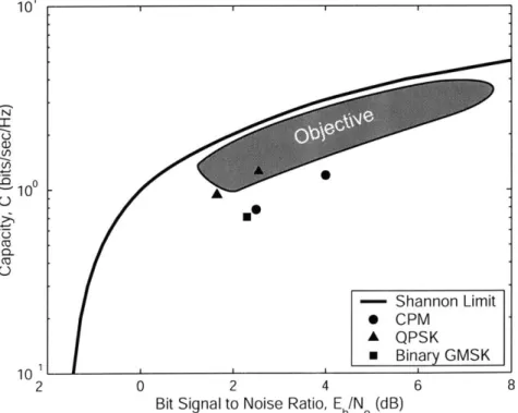
1-1 Comparison of Some Current Satcom Techniques with Shannon Capacity 13

2-1 A Basic Communication System . . . . 17

2-2 (8,4) extended Hamming code . . . . 19

2-3 Turbo Product Code Construction . . . . 21

2-4 Diagram of the Iterative Decoding Process . . . . 27

2-5 Turbo Product Code Performance Curves . . . . 27

2-6 (64,57)2 TPC Performance Curves with Error Bars . . . . 29

3-1 Example EXIT Chart and Decoding Trajectory . . . . 31

3-2 Iterative Decoder for Serial Concatenated Codes . . . . 32

4-1 Iterative Decoder for Turbo Product Codes . . . . 39

4-2 ten Brink's Iterative Decoder for Turbo Codes . . . . 40

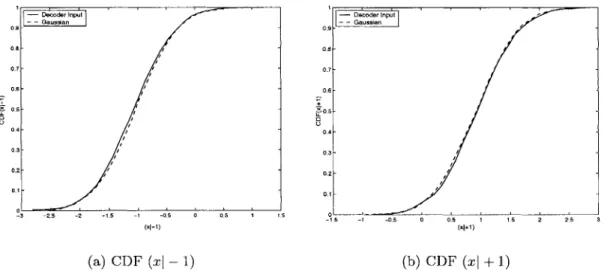
4-3 Decoder Input Bits Conditioned on X = -1 and X = +1 for BPSK in AWGN at Eb/NO = 2.5 dB . . . . 42

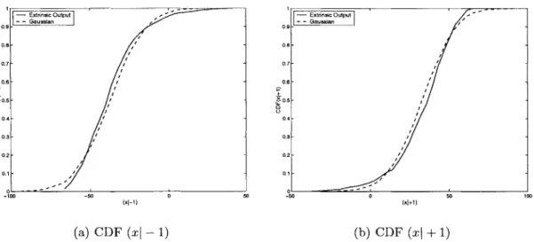
4-4 Extrinsic Output Conditioned on X = -1 and X = +1 for BPSK in AWGN at Eb/NO = 2.5 dB . . . . 43

4-5 Extrinsic Output Conditioned on X = -1 and X = +1 for GMSK in AWGN at E/No = 3.0 dB . . . . 43

4-6 EXIT Chart Development Example . . . . 45

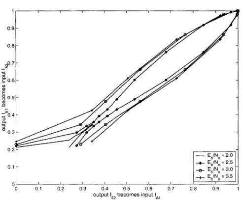
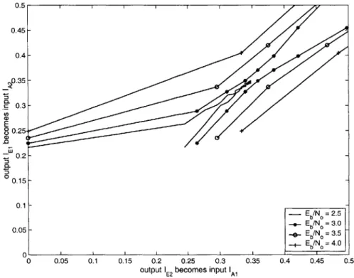
5-1 EXIT chart for the (64, 57)2 TPC . . . . 48

5-2 Close-up view of the transfer characteristics for the (64, 57)2 TPC . . 49

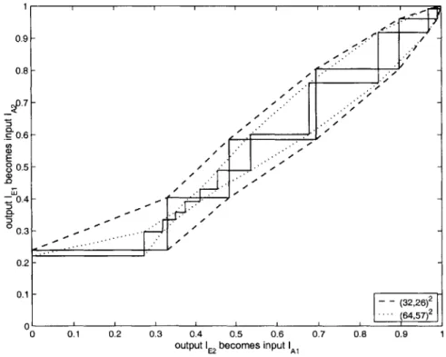
5-4 EXIT chart for the (64, 57)2 and (32, 26)2 TPCs at Eb/N, = 2.5 dB 52 5-5 EXIT chart for the (64, 57) x (32, 26) and (32, 26) x (64, 57) TPCs . 53 5-6 Performance Curves of the Non-square codes with BPSK in AWGN 54

5-7 EXIT chart for the (64, 57)2 TPC . . . . 55

5-8 Close-up view of the transfer characteristics for the (64, 57)2 TPC . . 56

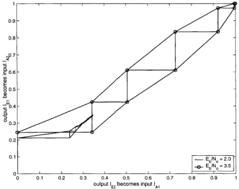
5-9 EXIT chart for the (64, 57)2 TPC at Eb/N, = 3.0 and 4.0 dB . . . . . 56

5-10 EXIT chart for the (64, 57)2 and (32, 26)2 TPCs at Eb/N = 3.5 dB . 57 5-11 EXIT chart for the (64, 57) x (32, 26) and (32, 26) x (64, 57) TPCs . . 58

5-12 Performance Curves of the Non-square codes with GMSK in AWGN . 59 6-1 Decoder Input Bits for the Rayleigh Channel Conditioned on X = -1 and X = +1 at E/N = 7.5 dB . . . . 62

6-2 Extrinsic Output for the Rayleigh Channel Conditioned on X = -1 and X = +1 at E/N = 7.5 dB . . . . 63

6-3 EXIT chart for the (64, 57)2 and (32, 26)2 TPCs . . . . 64

6-4 EXIT chart for the (64, 57) x (32, 26) and (32, 26) x (64, 57) TPCs . . 65

6-5 Performance Curves for the Non-square codes with BPSK in Rayleigh fading . . . . 66

6-6 EXIT chart for the (64, 57)2 and (32, 26)2 TPCs at Eb/N, = 6.0 dB 67 6-7 EXIT chart for the (64, 57) x (32, 26) and (32, 26) x (64, 57) TPCs . 68 7-1 (16, 11)3 TPC with BPSK in AWGN at Eb/N, = 1.0 dB . . . . 70

7-2 (16, 11)3 TPC at Eb/N, = 1.0 dB, front view . . . . 71

7-3 EXIT Chart for the (16, 11)3 TPC with BPSK in AWGN at Eb/N, = 1.0 d B . . . . 72

7-4 EXIT Chart for the (16, 11)3 TPC with BPSK in AWGN at Eb/N = 2 .0 d B . . . . 72

7-5 EXIT Chart with GMSK in AWGN at Eb/N = 1.0 dB . . . . 74

7-6 EXIT Chart with GMSK in AWGN at Eb/N = 2.0 dB . . . . 75

7-7 EXIT Chart in Rayleigh fading at Eb/N = 1.0 dB . . . . 76

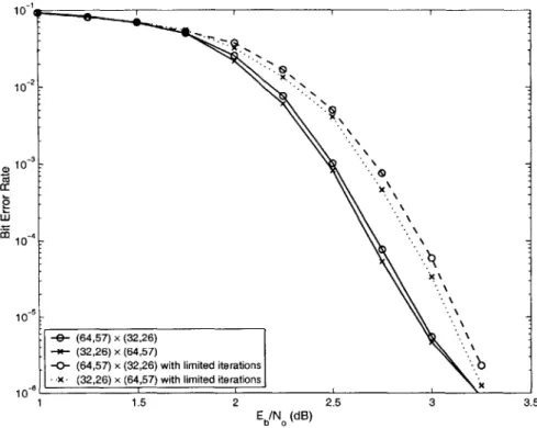
8-1 Predicted and Simulated BER curves for the (32, 26) x (64, 57) TPC .

8-2 EXIT chart with BER contours in AWGN . . . .

8-3 Predicted and Simulated BER curves for the (64, 57)2 TPC . . . .

8-4 Predicted and Simulated BER curves for the (16, 11) x (32,26) x (8,7)

TPC... ...

8-5 Predicted and Simulated BER curves for the (32, 26) x (64, 57) TPC .

EXIT chart with BER contours in Rayleigh Fading . . .

Convergence Thresholds versus Code Rate . . . .

Performance Curves with AWGN . . . .

Performance Curves for the (16, 11)3 TPC . . . .

Convergence Thresholds versus Iterations to Decode . . .

(32, 26) x (16, 11) x (8, 7) with GMSK in AWGN . . . . (16, 11) x (32,26) x (8, 7) with GMSK in AWGN . . . . (32, 26) x (16, 11) x (16,15) with GMSK in AWGN . . . (16, 11) x (32, 26) x (16,15) with GMSK in AWGN . . . (32, 26) x (16, 11) x (8, 7) with GMSK in Rayleigh fading

(16, 11) x (32, 26) x (8, 7) with GMSK in Rayleigh fading

81 81 83 84 86 87 90 91 92 . . . . 97 . . . . 98 . . . . 99 . . . . 99 . . . . 100 . . . . 101 . . . . 102

9-8 (32, 26) x (16, 11) x (16,15) with GMSK in Rayleigh fading . . . . 9-9 (16, 11) x (32,26) x (16,15) with GMSK in Rayleigh fading . . . . 9-10 Performance Curves with GMSK in AWGN . . . . 9-11 Performance Curves with GMSK in Rayleigh fading . . . .

10-1 Comparison of Some Current Satcom Modulation and Coding Schemes

with Shannon Capacity . . . .

8-6 8-7 8-8 8-9 9-1 9-2 9-3 9-4 9-5 9-6 9-7 102 103 104 105 109

List of Tables

8.1 Comparison of the predicted and simulated BER values for the (32,26) x

(64, 57) TPC at Eb/NO = 2.5 dB . . . . 82

8.2 Comparison of the predicted and simulated BER values for the (32, 26) x (64, 57) TPC at Eb/No = 7.0 dB . . . . 87

8.3 Convergence results for Two-Dimensional TPCs in the AWGN channel 88 8.4 Convergence results for Two-Dimensional TPCs in the Rayleigh channel 89 8.5 Convergence results for the (16, 11)3 TPC . . . . 89

9.1 Constituent Codes Available . . . . 94

9.2 Rate One-Half Codes . . . . 94

9.3 Convergence results for the AWGN channel . . . . 95

9.4 Convergence results for the Rayleigh channel . . . . 96

9.5 AWGN Results Summary: Number of Full Iterations to Decode . . . 99

Chapter 1

Introduction

In digital communications, several aspects must be considered when designing a for-ward error correcting code within a defined system. Some of these aspects include the code's block size and rate, the decoder's complexity of implementation, and finally the performance of that code. In general, we wish to maximize the performance and data rate of the code, while minimizing the complexity and size of the code. The above factors are especially true in the area of satellite communications where

on-board resources, such as power, weight/mass, spectrum allocation, and bandwidth may also be limited. Above all, the communication system must be reliable. Our ability to both accurately and quickly transmit large amounts of information over some distance determines the reliability of the communication system. We use for-ward error correction (FEC) in satellite communications to improve our performance, and thus increase the reliability of our communication system.

There has been a large focus on finding error correcting codes to meet our com-munication needs. During the 1990s, concatenated convolutional codes with iterative decoding, or turbo codes, were found to perform well. However, a high degree of complexity is needed to decode these codes [4]. In recent years, turbo product codes

(TPC) have also performed well without the high complexity of decoding required of the turbo codes [7]. To meet the goals of good performance, low complexity, and increasing reliability we want to use the best code for our defined system.

proposed tracking the evolution of the density of the information messages through the

decoding process. In [17] and [18], ten Brink extended the ideas of density evolution to the Extrinsic Information Transfer (EXIT) chart. The EXIT chart examines the evolution of the mutual information between the extrinsic information and the source

bits from one iteration to the next. He showed that the EXIT chart could not only be used to analyze the decoding process, but could also be used as a tool aiding the search to determine good codes for a given system.

1.1

Channel Capacity

In addition to meeting the power, space, and bandwidth requirements of a given communication system, one of the primary goals of coding is to maximize our use of the communication channel. In general, the channel capacity C is

C = max I(X; Y) (1.1)

where I(X; Y) gives the information gain between the transmitted signal X and the received signal Y [12]. This information gain is the mutual information between X and Y and is defined as

I(X; Y) = y) log Yp(x, ) (1.2)

where r = 2 for a binary system, p(x, y) is the probability of the x and y occurring jointly, and p(x) and p(y) are the probabilities of x and y occurring individually. The channel capacity C gives the maximum amount of information for a given channel [12]. The capacity of the channel is further defined to be the maximum rate at which

error-free communication exists, and is often referred to as the Shannon Limit. The maximum rate is usually measured in bits per second.

Gaussian noise (AWGN) channel,

C

R

s

log

( +

bits/sec/Hz.

(1.3)

The channel capacity C is a function of the bandwidth W and the information bit

energy to noise density ratio

[14]. By setting

where R is the code rate,

and using Equation 1.3, we plot the Shannon limit as a function of Eb/N in Figure

1-1. The ratio R/W of code rate to bandwidth is the bandwidth efficiency, which is

upper bounded by the Shannon Limit [14].

In Figure 1-1, as you move to the left on the x-axis with reduced Eb/N, the code

is more power efficient. The code is more bandwidth efficient as you move up along

the y-axis. We desire a code that is not only power efficient, but bandwidth efficient

as well. The desired performance area lies just below the Shannon Limit curve in the

upper left section of the plot. This area is highlighted in the figure.

10 1 100 10 1 2

I

Bit Signal to Noise Ratio, Eb/N (dB)

6 8

Figure 1-1: Comparison of Some Current Satcom Techniques with Shannon Capacity

Also shown are several codes, with associated modulation schemes, being

consid-I C-) a, C,) .0 U C-) CO 0~ CO U

Mow

ered for use in satellite communications. These codes include rate 1/2 and 2/3 turbo codes with quaternary phase-shift keying (QPSK) modulation and continuous phase modulation (CPM), and a rate 1/2 turbo code with binary Gaussian minimum-shift keying (GMSK) modulation. The Eb/N values are those required for a bit error rate

(BER) of 10-. For our purposes, we use the Eb/N required to obtain a BER of

10-5 as our performance measure, and the smaller the Eb/N value, the better the

performance of the code.

1.2

Objective

As shown in Figure 1-1, these codes and modulations have left room for improvement. We will examine TPCs to fill in some of those gaps. The examination will involve analyzing the TPC decoder developed by Advanced Hardware Architectures, Inc.

(AHA) and Efficient Channel Coding, Inc. (ECC), with AHA the hardware developer

and ECC the software developer. The EXIT chart method developed by ten Brink in [17, 18] will be used in this analysis.

There are several goals of this examination. The examination will cover the perfor-mance of the code in the AWGN environment and the Rayleigh fading environment, indicative of satellite and terrestrial wireless communication links as well. Also, we will use the results to determine if the common code combinations are in fact good codes, or which code performs best with a limited number of iterations. Finally, we will use our density evolution results to aid in the design of even better performing TPCs.

We were successful in extending the EXIT chart from turbo codes to TPCs. Also, the EXIT chart analysis was performed for both two-dimensional and three-dimensional TPC structures. This examination included binary phase-shift keying (BPSK), Gaussian minimum-shift keying (GMSK), and a fast Rayleigh faded chan-nel as well as the AWGN chanchan-nel. Finally, we verified the use of the EXIT chart as a code design tool to compare various rate one-half codes.

information on relevant error correcting codes, modulation schemes, and decoding. Chapter 3 will summarize ten Brink's previous applicable work for turbo codes. The details of our application of ten Brink's methods will be given in chapter 4. Chapters

5 and 6 will cover results of the density evolution analyses in the AWGN channel

and the Rayleigh fading channel, respectively. Chapter 7 will extend these analyses to multidimensional codes Chapters 8 will summarize certain results by comparing BER predictions and convergence analysis. Chapter 9 will use the EXIT Chart in a code design example. Finally, chapter 10 will give our conclusions and suggestions for possible future work.

Chapter 2

System Model

A typical communication system with forward error correction is shown in the block

diagram in Figure 2-1. The system begins with an information source which supplies

the message to be transmitted to the destination at the termination of the system. The message can be in any form, but for our purposes we will restrict our discussion to digital binary information sources. The information message first enters the encoder.

The encoder transforms the message into an encoded sequence of code words. These code words then enter the modulator. The modulator converts the code words into a waveform, or signal, for transmission through the communication channel. The chan-nel degrades the signal by adding noise and possible distorting the signal. Typically, the noise is AWGN, but the signal can also suffer from fading in the channel. Fading is common in terrestrial wireless and some satellite communication channels.

After passing through the channel, the received signal enters the demodulator. The demodulator performs the opposite function of the modulator by converting the

signal back into code words. The code words then enter the decoder. The decoder transforms the code words back into an information message. This is the opposite function of the encoder. Finally, the received information message reaches the

destina-tion. If the received message is the same as the transmitted message, the transmission is considered a success. Otherwise, the transmission is said to be in error, with the error rate given in terms of BER.

trans-Transmitter

Information _Encoder

Modulator Source

Channel

Destination Decoder Demodulator

-Receiver

Figure 2-1: A Basic Communication System

mitter functions. Similarly, the functions which occur after the channel can be grouped together as receiver functions. The following will discuss the transmitter

and receiver functions in further detail. Sections concerning the encoding, modula-tion and demodulamodula-tion, channel statistics, and decoding will be covered.

2.1

Encoding

FEC is the concept of applying some form of redundancy, or coding, to the information

we wish to transmit prior to the data being transmitted. This redundancy allows

for the detection and correction of transmission errors at the receiver [13]. Error correcting codes accomplish the goals of FEC. We will consider only binary codes in our examination; that is codes composed solely of the binary elements, or bits, 0 and 1. This section will review some basic error correcting codes, including linear block codes and convolutional codes. Turbo codes and turbo product codes will be addressed as well.

2.1.1

Error Correcting Codes

The most basic class of error correcting codes is the binary block code. A binary block code consists of the set of all fixed-length vectors known as code words. The code maps information bit sequences of length k to code words of length n > k such that

there are 2 k code words in the code. Each code word has n total bits. In systematic

codes, k bits are information bits, and the remaining n - k bits are called parity

bits. For an (n, k) binary block code, if all 2 k length n linear combinations of the

bits are linearly independent, we say that the code is an (n, k) binary linear block

code. Finally, the code rate is defined as R = k/n. This rate gives the number of

information bits per transmitted symbol, or code word [13, 14].

A useful property of binary linear block codes is the Hamming distance of the code.

The Hamming distance between two code words equals the number of corresponding positions where the two code words differ [14]. The minimum distance between any two code words in the code is denoted as dmin. The minimum Hamming distance of the code determines the code's error correcting capability [2]. For an (n, k) binary

linear block code with minimum distance dmin, the code can detect up to (dmin - 1)

errors. However, the same code is capable of correcting

[l(dmin

We will concentrate our discussion on a few types of block codes: single parity check codes, Hamming codes, and extended Hamming codes. These codes are fairly simple and straightforward to use, and are the constituent codes from which the TPCs used in this analysis will be constructed.

The first type of linear block code we will consider is the single parity check (SPC) code. We define SPCs such that

(n, k) = (m, m - 1) (2.1)

where m is any positive integer, however, we will restrict our attention to codes where

m is a power of two. SPCs are formed by first taking m - 1 binary information bits.

Then, the number of ones in the information bits are counted and an overall parity

bit is appended such the total number of ones in the code word is an even number. These codes have a minimum distance of two. Therefore, they can detect one error in a code word, but cannot correct any errors in a code word.

A second type of linear block code is the Hamming code. A Hamming code is

defined such that

(n, k) = (2m - 1, 2m - 1 - m) (2.2)

where m is any positive integer. These codes have a minimum distance of three and can detect up to two errors and correct one error per code word. A third type of linear block code is created by adding an overall parity bit to the Hamming code. This new code is the extended Hamming code. These codes have a minimum distance of four and can now detect up to three errors, but they can still only correct one error per code word. Figure 2-2 shows an (8, 4) extended Hamming code which has four information bits I and four parity bits P.

I I I I P P P P

Figure 2-2: (8,4) extended Hamming code

A second class of codes are convolutional codes. Like linear block codes, the (n, k)

representation is used where each code word has n total bits and k information bits. However, convolutional codes have memory. For a convolutional code with memory m, the current code word depends not only upon the current k information bits, but

upon the previous m information bits as well. The code rate is again R = k/n [13].

Typically, k and n are smaller for convolutional codes than for block codes.

Concatenated codes are formed as the result of combining two or more, separate codes so that a larger code is formed [14]. Either the block codes or convolutional codes mentioned previously may be concatenated together. Turbo codes are one type of concatenated code where the constituent codes, which are convolutional codes, are separated by a non-uniform interleaver. These codes typically perform quite well by performing close to the Shannon Limit at low bit error rates. However, these codes

require a high level of decoding complexity [4].

In recent years, a new type of error correcting code has created much interest. These codes have also performed well, but without the same high-degree of

de-coding complexity as turbo codes. This class of codes is known as turbo product codes (TPC). While TPCs have recently gained interest due to the iterative decoding method introduced by Pyndiah in [15], Elias first mentioned the idea of such a block

product error correcting code in 1954 [8).

2.1.2

Product Code Encoding

A TPC is a multidimensional array composed of linear block codes along each

di-mension, usually resulting in a two- or three-dimensional code. A two-dimensional code is encoded by using one linear block code along a horizontal axis and another along a vertical axis [4]. When encoding higher dimensional codes, the same pro-cess is used except additional axes are added until the higher dimension is reached. The constituent codes are usually comprised of extended Hamming codes or single

parity check codes. The use of such codes helps to keep the encoding and decoding complexity low [7, 2].

As an example, we will describe the encoding of the (8, 4)2 two-dimensional TPC. Since the two constituent codes have the same length, the resulting TPC will be square. The (8,4) code is an extended Hamming code that has four information bits and four parity bits (see Figure 2-2). The TPC is encoded by building first along

one axis and then along the second. The resulting TPC is an 8 x 8 matrix, shown in Figure 2-3, with I being an information bit and P being a parity bit. PH are the parity bits for the horizontally constructed code words, Pv are the parity bits for the vertically constructed codewords, and PVH are the parity bits of the parity bits [7, 2].

These values of PVH will be the same regardless of which axis is used to computer

I I I I PH PH PH PH

I

I

Figure 2-3: Turbo Product Code Construction

2.2

Modulation and Demodulation

In certain systems, especially the next generation satellite systems, the bandwidth available is limited. By using an appropriate modulation scheme, we can use the allocated bandwidth more efficiently. This section will review the two forms of modu-lation used in our examination of TPCs. The first is BPSK and the second is GMSK. While GMSK is a bandwidth efficient modulation used in the communication systems

of interest, BPSK will be used as a benchmark for performance comparisons because it is a standard modulation with straight forward analysis.

2.2.1

Binary Phase-Shift Keying

BPSK is one form of pulse amplitude modulation (PAM) and is relatively simple to implement. For an encoded code word x, the bits {0, 1} are mapped to {-1, +1}. This modulation scheme requires a large amount of bandwidth, and as a result is not very bandwidth efficient, with a 99 percent bandwidth of 1. The transmitted signal is

s(t)

A sin(wot + #)

(2.3)

where

#

The signal may be demodulated by performing matched filter detection and mak-ing a binary decision on the filter output. This process is known as hard decision

negative, the demodulated bit is a -1, and if the sign is positive, the demodulated bit is a +1 [14].

2.2.2

Gaussian Minimum-Shift Keying

GMSK is a form of continuous phase modulation (CPM) which gives the signal a continuous phase and constant envelope. The transmitted passband signal is

s(t) = Re{sbb(t) exp{j2rfj} (2.4)

where sbb(t) is the complex baseband envelope of the signal s(t), and

f,

frequency. The baseband envelope is

2ER

_iT'

Sbb(t) T

exp j2,rh

aq

(2.5)

P

where E is the signal energy, T is the pulse width, and R is the fractional pulsed

chipping rate, with R = 1 for GMSK. ao takes values from the set {-1, 1} with the

phase transition

I

t

Q(ti)

Q(ct

exp(-or

2

_/2)t2

_exp(-

_/2)t2

lq(t)

(2.6)

2 2Tp 2T,

V'

where B is the 3 dB bandwidth of the Gaussian filter,

Q

a

27rB/v%

The modulation occurs when the encoded code words are sent through a pulse shaping filter, the output of which modulates the phase of the transmitted signal. An interleaver reduces the amount of inter-symbol interference present in the signal after demodulation. Demodulation may be accomplished with an application of the soft output Viterbi algorithm (SOVA). While GMSK is more complex to implement than BPSK, it has two important advantages. First, GMSK is much more bandwidth efficient than unfiltered BPSK, with a 99 percent bandwidth of 0.7. Second, additional performance gains can be made through the use of the Viterbi algorithm in the

demodulation of the received signal.

2.3

Channel Statistics

The channel represents the path the signal takes to get from the transmitter to the receiver. For a land-based telephone system, the channel is a wire. A wire can be easily modeled. However, for terrestrial wireless and satellite communication systems, the channel is free space. Due to many factors, including the natural environments, buildings, and other users, the channel is more difficult to model. Usually, we wish to model an average channel, and we use AWGN for this purpose. White noise has a flat power spectral density and is uncorrelated with respect to time. However, when channel is faded, the noise is characterized by a non-Gaussian statistic. In a fading channel, the noise does not have a constant power spectral density and is both time varying and correlated with respect to time. When modeling such channels, we use a statistic such as the Rayleigh probability density function (PDF). The following will

discuss both AWGN and Rayleigh channel statistics.

2.3.1

Additive White Gaussian Noise Channel

The AWGN channel is the standard channel used when designing communication systems. The noise is characterized by the Gaussian PDF as

p(x) = eX 2/2,2 (2.7)

where a.2 is the variance of the zero-mean noise. White noise is also defined to have

a constant, or flat, power spectral density over the entire frequency band [14]. For

AWGN, the one-sided noise spectral density is given as N0 = 2a.2, and the information

bit energy to noise density ratio is given as Eb/N, in dB.

that the resulting complex received signal is given as

z. = xe + nc (2.8)

where zc is the received complex signal, x, is the modulated complex signal, and n, is

the complex AWGN. Both the real and imaginary components of n, are independent

zero-mean Gaussian random variables with variance ca.

2.3.2

Rayleigh Faded Channel

The Rayleigh PDF is usually used to model those channels which are characterized

by several multiple paths with no significant line of sight (LOS) path present. The

fade is Rayleigh distributed according to

prayi(a) =

ae-a2/2,2

072

where a is the magnitude of the fade and u2 _{is the variance, which is different from}

the variance of the AWGN.

In our analysis, the modulated signal was multiplied by the Rayleigh distributed fade and then complex AWGN was added to the signal. The fading envelope was

generated using two independent Gaussian random variables, x1 and X2, as

a(t)

=

The resulting complex received signal can be expressed as

zc = ac - xc

+

where z, is the complex received signal, ac is the complex Rayleigh envelope as in Equation 2.10, xe is the transmitted signal, and n, is the complex AWGN.

Rayleigh fading can be applied in one several ways, and two methods will be described in the following. First, we can model a slow fading scenario. This is when

the duration of the fade is slow with respect to the signaling interval, or symbol duration, and was modeled by applying the same fade over an entire block of data. This will be referred to as block fading. A second application of Rayleigh fading is usually in a fast fading scenario. Since the duration of the fades are fast with respect to the signaling interval, or symbol duration, we modeled this fade by applying an independent Rayleigh distributed fade to each symbol within a given block. This will be referred to as symbol fading.

2.4

Decoding

Decoding estimates which code word was transmitted through the communication system. Several decoding methods exist - ranging from the simple, hard decision decoding, to the complex, soft input-soft output (SISO) iterative decoding. Our desire to maximize performance while minimizing complexity and the code structure determine which decoding method is used. The following will discuss hard decision

decoding and soft decision and SISO iterative decoding.

For a system with inputs

{

the received bits. For our purposes, we used the {0, 1} -+ {-1, +1} modulation, and

as a result, if the sign of the received bit is negative, the input to the decoder is a -1, and if the sign is positive, the input to the decoder is a +1. The decoder chooses the code word that is closest in Hamming distance to the received word. If the decoded word matches the transmitted word, then the block was decoded correctly, otherwise

the block is said to be in error.

In contrast to the hard decision decoder, a soft decision decoder uses the sign of the received bits as well as additional soft input information to make the decoding

decision. This additional information is usually given as reliability information which gives a confidence value regarding the hard decision. One decoding rule that is used in soft decision decoding is the maximum likelihood (ML) decoding rule, which min-imizes the probability of error by maximizing the probability of the received word given a transmitted word, or P(rjv), where r is the received code word and v is the

transmitted code word [13]:

argmax P(r

Ivi)

where ri and vi are the bits of the code words r and v and we assume that the received symbols are independent. ML decoding is considered to be an optimum decoding rule

[13].

Even though soft decision decoding is more complex to implement than hard decision decoding, it is often used due to the significant performance improvements that result. However, to further improve performance iterative decoding algorithms have been developed. These algorithms make use of not only soft input information, but soft output information as well. For more information on Pyndiah's, Chase's, and an application of Viterbi's iterative decoding algorithms, please refer to [15], [5], and [11], respectively.

In the following examination of TPCs, Thesling's cyclic-2 pseudo maximum like-lihood decoding algorithm will be used [19]. This algorithm is sub-optimal, but for TPCs composed of extended Hamming codes and single parity check codes with BPSK in AWGN, the algorithm performs almost at the true correlation decoding value [7]. The first step of this algorithm involves making a hard decision on the received signal. The sign and magnitude, or reliability, information that results are then sent through the iterative process. The rows are decoded first with the soft output adjusted by a weighting function. This adjusted soft output information then becomes the soft

input to the column decoder. The soft output from the column decoder is adjusted

by a weighting function as well. The weighting function following each axis iteration

need not be the same; the parameters of these functions are controlled by an opti-mized feedback value [3]. The extrinsic soft output and input information, noted as

softrow,in, softrow,out, softcolumnin, and softcolumnout in Figure 2-4, are passed between the two decoders in an iterative fashion. The decoding process continues until no further corrections can be made to the code word, or until the maximum number of iterations has been reached [2]. For our purposes, the weighting function

is considered to be part of the decoder function and is not shown in the figure.

Channel Input soft row, out Decoder Output

Row Decoder Column Decoder

Soft _{column, out}

Sotrow, in _S ILIT lMn, 11n

Figure 2-4: Diagram of the Iterative Decoding Process

Using iterative decoding, various two- and three-dimensional TPCs with code rates of 1/3 to 4/5 have performed within 2.5 dB of the Shannon Limit at a bit error

rate (BER) of 105 . Figure 2-5 shows the bit error rate performance curves for a

two-dimensional TPC in a BPSK modulated AWGN channel. The given results were achieved using only a few iterations. On average, this TPC was decoded in four to six complete iterations, with a complete iteration including both one row and column decoding. This code will be analyzed further in later sections of this thesis.

100 10-1 10-2 (1) -3 1 10 - -4 105 10-0 1 2 3 4 5 6 E /N (dB) 7 8 9 10 11

Figure 2-5: Turbo Product Code Performance Curves

(64,57) x (64,57) Uncoded BPSK .... _{Shannon Limit}

The coding gain is based upon a code's performance improvement over the perfor-mance of uncoded data with similar conditions. Figure 2-5 not only gives an uncoded

BPSK curve, but shows the Shannon Limit for codes of rate 4/5, which is at an

Eb/N, of 2 dB [7]. The coding gain is upper bounded by the distance from the

un-coded curve to the Shannon Limit for the code at a given error rate. For the codes of rate 4/5, the maximum coding gain is 7.5 dB at the error rate of 10-5. With BPSK modulation, the (64, 57)2, rate 0.793 TPC has a coding gain of about 6.3 dB at the error rate of 10-5. In contrast, the difference from the Shannon Limit curve to the code's performance curve shows coding, or power, inefficiency. For this code, we have an inefficiency of about 1.2 dB.

To give a measure of the accuracy of the performance curves used throughout the remainder of the thesis, error bars showing the 95 percent confidence intervals are shown for the curve for the (64, 57)2 TPC in Figure 2-5. However, because the error bars are quite small in the preceding figure, a closer view of the BER curve is shown in Figure 2-6. As shown, the confidence interval is quite close to the BER curve, increasing only slightly at the lowest error rates plotted. These intervals are

representative of the accuracy of the data used throughout this thesis.2

In the next chapter, we will begin our discussion density evolution and EXIT charts by examining ten Brink's methods for convolutional codes.

2

This interval size assumes that all bit errors are independent, when they actually occur as part of an errored block. Thus, the error bars illustrated are somewhat optimistic.

0 -- 95 % confidence intervals - - (64,57) x (64,57) 10-10-2 - 10-10- - - 10-107 1.5 2 2.5 3 3.5 E b/N (dB)

Chapter 3

ten Brink's Methods for Turbo

Codes

We have briefly examined how TPCs are constructed and decoded. We have also been given some preliminary performance results. Next, an analysis method is needed to determine which codes will perform best while meeting the system requirements. One such method is density evolution. Density evolution tracks the extrinsic information of the decoders from iteration to iteration in order to map the overall convergence of the decoder. The extrinsic information is the soft output information gained dur-ing the iterative decoddur-ing process. Divsalar, Dolinar, and Pollara applied a density evolution analysis to turbo codes and low density parity check codes. They tracked the evolution of the signal-to-noise ratios (SNR) of the decoders to analyze the iter-ative decoding process [6]. In [17] and [18], ten Brink examined the evolution of the extrinsic information through its mutual information using an Extrinsic Information Transfer (EXIT) Chart. A common goal of both analyses was to use their density evolution method to aid in code design for iteratively decoded systems. We chose to use ten Brink's methods in our density evolution analysis.

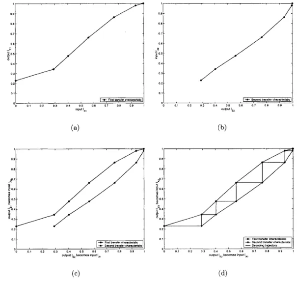
In his examination, ten Brink used the EXIT chart to visually demonstrate the evolution of the extrinsic information through a soft input/output iterative decoding process. By using the standard deviation of the soft input and soft output information, ten Brink calculated the mutual information between the extrinsic information and

the transmitted bits at the various stages of the iterative decoding process. For each constituent decoder, a plot of the mutual information at the input versus the mutual information at the output represents its transfer function. By plotting the transfer functions of the two decoders against each other, he was able to generate the EXIT chart[17, 18].

Using the EXIT chart, one could then plot the decoding trajectory. The decod-ing trajectory shows the evolution of the mutual information through the decoddecod-ing process as a block is completes decoding. The trajectory is a stair-step like line con-necting the two transfer characteristics. However, if the two transfer functions cross, we are unable to plot the decoding trajectory, and we know that that block was not decoded correctly. In addition, ten Brink showed that it was also possible to use the EXIT charts to predict the BER at low Eb/N values [18]. Finally, he listed several possible applications of the EXIT chart, including using it as a tool for code design.

0.9- 0.8-7 -0.6 -E OL0.5 --0.4 - 00.3-0.2

-0.1 - -0- First transfer characteristic

-I- Second transfer characteristic

- Decoding trajectory

0 0.1 0.2 0.3 0.4 0.5 0.6 0.7 0.8 0.9 1

output IE2 becomes input IAl

Figure 3-1: Example EXIT Chart and Decoding Trajectory

Figure 3-1 shows an EXIT chart for the (64, 57)2, rate 0.793 TPC using GMSK

correctly decode the block at this instance. The decoding trajectory is allowed to step through the tunnel created by the two transfer characteristics.

ten Brink developed his methods for examining the density evolution of an iterative decoding process using both serial and parallel concatenated turbo codes. Recently, in [10] his ideas have been applied to non-binary codes. In this thesis, his ideas will be applied to TPCs. However, we will first begin with an in-depth review of the process required to create an EXIT chart. The EXIT chart is a graphical description of the density evolution of the decoding process, and it is the primary tool that will be used for not only the density evolution analyses, but performance, or BER, analysis and convergence analysis as well. This section also sets up the required background and nomenclature used in the TPC analysis.

3.1

Mutual Information Analysis

3.1.1

The Iterative Decoder

Deinterleaver

Channel Z Channel

Input Inner D1 E1 I A2 - Outer Output

Decoder . _{Decoder D}

2

A1

Interleaver

Figure 3-2: Iterative Decoder for Serial Concatenated Codes

Figure 3-2 shows the serial iterative decoder for which ten Brink developed his analysis [17]. From this figure, we can see that a deinterleaver and an interleaver sepa-rate the inner and outer convolutional decoders. These decoders perform maximum a posteriori (MAP) decoding according the the Bahl-Cocke-Jelinek-Raviv (BCJR)

algo-rithm [17]. The decoding process begins when the noisy channel bits, Z, are input to the decoder. These bits are decoded first by the inner decoder, giving the soft output

D

information, D, minus any a priori input information A such that El = D, - A1

[17, 18]. This subtraction is necessary to determine exactly how much information

is gained as the bits pass through the individual decoder. El gives the extrinsic

in-formation of the first decoder and is the a priori input for the second decoder, A2.

Similarly, E2 = D2 - A2 is the extrinsic information of the second decoder and a

priori input to the first decoder. The process of passing the extrinsic information

from decoder to decoder continues until the decoding is completed, which is usually after a certain number of iterations or when the block is decoded to a codeword.

The variables Z,

E1, D

, A

,

[17, 18]. For the AWGN channel, the received signal, z, is given as

z = x + n (3.1)

where x are the transmitted bits and n is the additive noise. The noise n is also

Gaussian distributed with zero mean and o = N,/2. The L-values [17, 18] are then

calculated according to

p(zlx

=+1)

Z =

ln(

1)

p(zIX = -1)

where the conditional PDF of the noisy channel bits, Z, given the transmitted bits

X is

e-((2-X)2/2 n

p(zjX

x)

Using the conditional PDF and the Gaussian channel representation of Equation 3.1, the L-value representation can be simplified to

2 2

Z - . = 2 -(x + n). (3.4)

This representation can also be re-written as

Z = pz -x

+

where

pz = 2/an

and the noise nz is Gaussian with zero mean and variance

UZ = 4/on.

Finally, we can show that the mean and variance of Z are related by

2 cIZ I'Z 2 (3.5) (3.6) (3.7) (3.8)

This development of the received signal Z will be useful for later derivations [17, 18].

3.1.2

Mutual Information Calculations

ten Brink chose to model the a priori input to the individual decoders as an inde-pendent Gaussian distributed random variable A with variance o2 and zero mean

[17, 18]. As a result, it is possible to write the L-values A as

A

x

in accordance with Equation 3.5, and where x are the transmitted bits and nA is the additive Gaussian noise, with zero mean and variance o2. Following from modelling

A as Gaussian distributed and with pALA o/2, the conditional probability density

function of A given X becomes

e-(-X.U2/2)2/2U2

The mutual information is a measure of the gain in information due to the re-ception of a signal. This gain in information is found by determining the difference between the information uncertainty before, the a priori probabilities, and after the reception of the signal, the a posteriori probabilities [12]. A general representation

of this calculation is given in Equation 1.2. The mutual information I = I(X; A)

between the transmitted bits X and the a priori information A is found using the following

IA - E PA((IX = X) X g2 X=X) dPA (3.11) 2_=-00 PAx(W1 -- 1) pA(IX = 1)

Using Equation 3.10 and Equation 3.11, the mutual information IA becomes

+00 e-( /2)2 /22

IA(UA) = - (1 - log2[1 + e4])d< (3.12)

The mutual information is now given as a function of the standard deviation of the a priori input to the decoder [17, 18]. The mutual information is a monotonically increasing value that exists over the range 0 to 1, assuming equally likely binary source symbols, and where OA > 0 always. We can also abbreviate Equation 3.12 as

J(U)

o-).

Because IA is monotonically increasing, it is also reversible according to

oA J(IA)-

(3-14)

We can quantify the mutual information of the extrinsic output IE = I(X; E)

using a similar method. However, ten Brink did not assume that the extrinsic infor-mation is Gaussian distributed [18]. In his work, a Monte Carlo method was used to determine the distributions PE, and the mutual information IE is computed using

equation 3.12 with the derived PE in place a PA. As with the mutual information IA,

3.1.3

Transfer Characteristics

The transfer characteristics of the constituent decoders are found by viewing the

extrinsic output information IE as a function of the mutual information of the a

priori input IA and the signal power to noise density, Eb/No, such that

IE = T(IA, Eb/No). (3.15)

When the signal power to noise density is held constant, this relationship becomes

'E= T(IA). ten Brink was able to isolate his decoders so that he could independently

plot the extrinsic information transfer characteristics of the inner and outer decoders

for a given and constant Eb/NO. Using the inverse relationship between UA and

the mutual information 'A from Equation 3.14, ten Brink applied the independent

Gaussian random variable of Equation 3.9 to the decoder of interest. By choosing

the appropriate value of UA, the desired value of 'A could be achieved [17, 18].

In the plots of the transfer characteristics, the mutual information of the a priori input was plotted on the abscissa and the mutual information of the extrinsic output was plotted on the ordinate for the inner decoder. The axes are reversed for the second, or outer, decoder. These plots are the transfer characteristics of the individual decoders [17, 18]. Since the mutual information ranges from zero to one, the transfer characteristics will also range from zero to one. Finally, the transfer characteristics are monotonically increasing because the mutual information is also monotonically increasing.

3.2

The Extrinsic Information Transfer Chart

To plot the EXIT chart for a complete iterative decoding process, transfer charac-teristics for each of the decoders are used. The transfer characcharac-teristics for the first constituent decoder are plotted such that the input extrinsic information is on the abscissa and the output extrinsic information is on the ordinate. For the second de-coder, the axes are reversed. By plotting the two curves on the same diagram, we

create the EXIT chart [17, 18]. This axis swapping is necessary such that the extrinsic information and channel output of the first decoder I 1 becomes the a priori input

IA2 to the second decoder. Then, the extrinsic information and channel output of the second decoder IE2 becomes the a priori input IA, to the first decoder, and so on.

Please refer to Figure 3-1 on page 31 for an example of the EXIT chart.

The decoding trajectory can be added to the EXIT chart to show the evolution of the mutual information through the decoding process as a block is decoded. The trajectory is a stair-step shaped line connecting the two transfer characteristics. For a block to be decoded correctly, the decoding trajectory must span the range of the transfer characteristics, zero to one. We consider a decoding process to be complete and successful when the mutual information is monotonically increasing over the entire range 0 < IE < 1.

The key idea of the success of a decoding process is that the amount of mutual information must always increase from one half iteration to the next. As long as

IE2,n+1 > IE,,2, the iterations, and ultimately the decoding process, will proceed. If IE 2,n+1 i IE 2,n, the decoding process will not be able to complete [17, 18]. As a result, the two transfer characteristics will intersect, and the corresponding decoding trajectory will terminate at the point of intersection. The current block will not be decoded correctly because the decoding trajectory did not reach one, which is needed for the block to be complete decoding.

3.3

Additional Results

ten Brink continued his examination of turbo codes by using the EXIT chart to predict the BER for a code structure after any number of iterations [18]. ten Brink also applied his methods to a coherently detected, fully interleaved Rayleigh channel, including the BER prediction [18]. Finally, he listed several important additional

uses of the EXIT chart. These include using the chart as a design tool for iterative decoding schemes, including code searches, and using the chart to help gain insight into the convergence behavior of the iterative decoder [17, 18]. His methods for these

Chapter 4

Application of ten Brink's

Methods to Turbo Product Codes

While ten Brink developed the EXIT chart for turbo codes, the main target of the examination was actually the iterative decoder. In chapter 2, it was shown that TPCs are decoded using an iterative decoder. As a result, TPCs are an ideal extension for the EXIT chart analysis. In this chapter, we determine changes necessary due to the differences in TPC decoder structures as well as in the information available from the TPC decoder. Then, ten Brink's assumptions will be extended to TPCs. Finally, differences in the mutual information analysis and methods used for plotting the EXIT chart and associated decoding trajectory will be presented.

4.1

Iterative Decoder

Channel Input soft row, out Decoder Output

Row Decoder Column Decoder

Soft column, _out

sotrow, sof column, in