Deep learning approach to metagenomic binning

(1)

Deep Learning Approach to Metagenomic Binning

by

Ryan Kyong-doc Chung

Submitted to the Department of Electrical Engineering and Computer

Science

in partial fulfillment of the requirements for the degree of

Master of Engineering in Computer Science and Engineering

at the

MASSACHUSETTS INSTITUTE OF TECHNOLOGY

June 2018

c

○ Massachusetts Institute of Technology 2018. All rights reserved.

Author . . . .

Department of Electrical Engineering and Computer Science

June 1, 2018

Certified by . . . .

Bonnie Berger

Professor of Electrical Engineering and Computer Science

Thesis Supervisor

Accepted by . . . .

Katrina LaCurts

Chairman, Department Committee on Graduate Theses

(2)

(3)

Deep Learning Approach to Metagenomic Binning

by

Ryan Kyong-doc Chung

Submitted to the Department of Electrical Engineering and Computer Science on June 1, 2018, in partial fulfillment of the

requirements for the degree of

Master of Engineering in Computer Science and Engineering

Abstract

Understanding the diversity and abundance of microbial populations is paramount to the health of humans and the environment. Estimating the diversity of these popu-lations from whole metagenome shotgun (WMS) sequencing reads is difficult because the size of these datasets and overlapping reads limit what kinds of analysis we can do. Current methods require matching reads to a database of known microbes. These methods are either too slow or lack the sensitivity needed to identify novel species. We propose a convolutional neural network (CNN) based approach to metagenomic binning that embeds reads into a low-dimensional vector space based on taxonomic classification. We show that our method can get the speed and sensitivity necessary taxonomic classification. Our method was able to achieve 13% accuracy on identify-ing novel genus of bacteria as compared to 7% accuracy of k-mer embeddidentify-ing. At the same time, the speed of our method is within an order of magnitude of that of k-mer embedding, making it viable as a metagenomic analysis tool.

Thesis Supervisor: Bonnie Berger

(4)

(5)

Acknowledgments

To the Berger Lab:

Thank you all for the academic support throughout my time in the lab. Bonnie, thank you for the incredible kindness you have shown to me. Your guidance has lead me through some of the toughest times and decisions I have faced. My eternal gratitude goes out to Tristan who’s generosity of his time and talents cannot be un-derstated.

To my parents:

I can’t thank you enough for love you have shown towards me and the quiet sac-rifices you have made.

To my friends:

Thank you for keeping me sane on a daily basis. It’s been a whirlwind adventure, and I’m glad to have shared it with all of you.

(6)

(7)

List of Figures

2-1 Triplet Network . . . 19

2-2 Noise contrastive estimation . . . 21

3-1 CNN Embedding Model . . . 26

4-1 Training and Validation Results . . . 31

4-2 Embedding space and cluster breakdown for CNN and k-mer embeddings. 33 4-3 Read embedding comparison. . . 34

4-4 Embedding space and cluster breakdown for CNN and k-mer embed-dings on WMS dataset. . . 35

(10)

(11)

List of Tables

4.1 Modeling Results . . . 29 4.2 Runtime of Embedding algorithms . . . 36

(12)

(13)

Chapter 1 Introduction

A microbiome is a community of bacteria, fungi, archaea and viruses in the same environment. Understanding the taxonomy, or classification, of each organism in a microbiome is central to many biological and healthcare related questions. In fact, recent research suggests that the human gut microbiome is important for human health. A disfunctional microbial composition could lead to disorders such as irritable bowel syndrome (IBS) [24], asthma [8] and autism [4]. By understanding the diversity of the human gut microbiome, we can better characterize, diagnose, and develop personalized approaches to remedy these gut related diseases. Discovery of novel drugs and biomolecules, such as antibiotics, also hinges on homology based microbial analysis [2]. By forming an understanding of taxonomic space, we can search related microbes for potential therapeutic compounds.

1.1 Metagenomics

Diagnosis of gut related diseases and drug development are difficult because determin-ing the taxonomic composition of a microbial population directly requires isolatdetermin-ing and sequencing pure samples of each microbe [13]. Possibly the most important success in interpreting the diversity of these populations has been in the field of metagenomics. Metagenomics is the application of modern genomics techniques to the study of microbial communities in their natural environments without isolating

(14)

individual species [6]. By sequencing the bulk DNA we can quickly get an estimate of the diversity of a microbiome. The standard method for estimating diversity and abundance is amplicon sequencing. Amplicon sequencing uses primers to amplify a conserved region of the genome (e.g. the 16S rRNA gene). Homology within this re-gion is used as an indicator of taxonomy. By matching the gene variants to a reference database, we can identifying the taxonomic composition of a sample. This approach allows researchers to get a relative understanding of microbial populations. However, amplicon sequencing loses much subspecies and gene specific information [12].

High-throughput sequencing technologies have led to an explosion in the amount of microbiome sequencing data. These whole metagenome shotgun (WMS) sequencing datasets contain millions of short reads (25-300bp) sampled from the organisms in the community. Because this technology allows for high coverage of genetic regions, we get good resolution of genetic variants. Despite this clarity, the size of these datasets means that we cannot use many of the typical bioinformatic tools. The usual approach to shotgun sequencing data is to assemble these short reads by finding overlapping reads and merging them. Unfortunately, assembly typically fails on metagenomic data due to low read coverage or having reads that can map to multiple organisms in the population [18]. To make use of these sequenced genomic fragments, we can group reads by taxonomy (genus, species, strain) in a process called metagenomic binning. These taxonomically similar reads can be used in diversity analysis, genome assembly, or functional analysis of the microbiome [25].

1.2 Related Works

Current approaches to WMS sequence binning fall into two categories: (1) taxonomy dependent and (2) taxonomy independent. Taxonomy dependent methods align reads to the closest reference genome in the database using algorithms like BLAST [1], BWA [16] and Bowtie [15] or find the reference genome with the closest composition (e.g. k-mers or GC content) to the read [25]. Examples of taxonomy dependent binning include CLARK [21], Kraken [27] or PyloPythia [9]. Typically, these methods are

(15)

either too slow to analyze the large quantity of reads or are not powerful enough to understand the full diversity of these reads. On top of these issues, taxonomy dependent methods are unable to correctly classify reads from genes and species absent from the database.

Taxonomy independent methods, on the other hand, use clustering methods to determine similarity between sequences. Tools that fall into this category are Com-postBin [5], AbundanceBin [28], and VizBin [14]. Most of these methods also use k-mer composition or abundance to sort reads into clusters. Although these methods are not constrained by the quality and size of our reference genomes, they are unable to learn critical information from the taxonomy of fully sequenced organisms. Fur-thermore, discriminating reads based on k-mer counts is intolerant because k-mers require exact matches so they cannot represent mutations like mismatches or gaps well. To address this problem of intolerant k-mers, the tool Opal used locality sen-sitive hash functions to represent long but flexible k-mers concisely [18]. However, these methods still suffered from lack of sensitivity with this representation so it was unable to capture information at lower phylogenetic levels (species and strain). To generate a feature vector that better captures taxonomic information from a read, we opted to use neural networks.

1.3 Overview

In this thesis, we will improve on previous k-mer based techniques by using neural networks to embed reads into a learned vector space in which distance between em-beddings is predictive of taxonomic distance. By training a neural network to learn these embeddings we leverage the information from known microbial genomes and the speed of taxonomy independent methods. Using these embeddings we cluster reads based on taxonomic similarity and get taxonomic separation even for reads from taxonomic groups not present in the training set. We describes the architecture of our model, and the motivations for the design decisions made in Chapter 2. We then go on to describes the analysis of our model in chapter 3, as well as how the

(16)

optimizations discussed in section were implemented. Chapter 4 describes our results and conclusions from this project. Possible future expansions to the project are also discussed.

(17)

Chapter 2 Comparative Evaluation of

Metagenomic Binning

In recent years, deep neural networks have grown in popularity due to advances in hardware and innovation in network architecture. These advances have made neural networks a powerful tool capable of understanding complex distributions or classifying images. Since they can be formulated as simple matrix manipulations, high dimensional data can be processed quickly. In our particular application, we use a few neural network architectures to generate a low-dimensional representations, or embedding, of metagenomic reads that preserve taxonomic differences. The best network was then used to generate the read embeddings which were harnessed as features to cluster taxonomically similar reads. With these clusters, we can infer the abundance and composition of the populations it is drawn from.

2.1 Metric Learning

We want to use neural networks to learn a distance which preserves some conception of similarity between inputs. This problem has been studied extensively in the area of image recognition. In image recognition this similarity is determined by the class of the image (i.e. human, car, dog). They learn this distance metric using neural networks to embed the original input into an informative space that preserves these

(18)

similarities. In our problem, the distance metric we want to learn is taxonomic distance.

We embed metagenomic reads in a lower dimensional taxonomic space by training a neural network to determine if a read has the same label or not. In this binary classification problem, we can use the distance between embedded samples as an approximation of probability of being in the same class. The key concept in many metric learning approaches is to maximize the distance between the representations of data with different labels and minimize the distance between representations with the same label. These two competing forces allow samples to cluster and be represented in their own section of an embedding space.

One such metric learning approach uses the Siamese neural network [11]. This network has two subnetworks with shared parameters to process two inputs. In the original application, the network learns a low-dimensional representation of a large number of images. It does this by training the network to maximize a distance between the network embeddings of two samples with different labels. They showed that their network generalized well and could generate useful embeddings even for new data classes. Since the network was not trained to predict specific image classes, it was able to separate unseen images in different categories with no additional training.

In the same way, our metric learning approach does not directly use taxonomic labels so it is not strictly constrained as a classification problem. Instead, the neural network can learn an embedding space that separates reads based on taxonomic clas-sification. By training with enough species we show that this representation extends to unknown species.

2.1.1 Triplet Network

An improvement on this metric learning approach is the Triplet network which uses a comparison function to better optimize distance between different labels [10]. The Triplet network determines if an embedded sample is closer to another embedding with the same label or that of a different label (Figure 2-1). Formally, the network takes three inputs at each step. Two of the inputs have the same taxonomic label

(19)

Figure 2-1: The Triplet network takes three input reads with 𝑥+ _{and 𝑥 having the}

same label. The reads are mapped to an 𝑛-dimensional space with the same CNN (Net). The L2 distance between the two reads with the same label and the two with different is calculated. The comparator, which is MSE loss function, is used to make the distance between the different labeled reads large and the distance between the same labels small.

(𝑥 and 𝑥+_{) and one has a different label (𝑥}−_{). A CNN encoder converts all three}

samples into an 𝑛-dimensional feature vector. The comparator function takes the distance (the L2-norm of the difference) between the embedded features of the two samples that are the same (CNN(𝑥) and CNN(𝑥+)) and the embedded features of the two of the samples that are different (CNN(𝑥) and CNN(𝑥−)). Here, we want to minimize the distance between the representations of the same labeled reads and maximize the difference between the representations for the different labeled samples. We do this by taking the softmax of these two norms and pushing it to (0, 1) with the Mean Squared Error (MSE) objective function. The softmax function makes the norms in the range (0,1) and allows us to treat this as a the probability of a two-class problem. Here the network is giving a probability that one read is more similar to one than another.

(20)

2.2 Noise-Contrastive Estimation

Noise-Contrastive Estimation (NCE) is used in NLP to generate word embeddings and the popular tool word2vec uses an objective function based on NCE [19]. With this tool, a neural network embeds the word token as a vector and uses gradient descent to maximize the similarity (dot product) between word vectors that appear in the same context. Although NCE uses a technique similar to that of triplet networks it solves a different problem [20]. In tese types of problems, we want to estimate the likelihood of a sample 𝑥 being generated from a label class 𝑙 (taxonomy in our case).

𝑃 (𝑥|𝑙) = 𝑃 (𝑥, 𝑙) 𝑃 (𝑥) = 𝑃 (𝑥, 𝑙) ∑︀ 𝑥∈𝑋𝑃 (𝑥, 𝑙) (2.1)

In the problem of binning reads, normalizing these probabilities requires summing over the space of short 200bp reads. This space has 4200 _{= 2.6𝑥10}120 _{combinations.}

Here, summing over all possible samples is computationally infeasible. We can instead solve a different problem: training a model to differentiate between samples from the empirical distribution or from a noise distribution [7]. Instead of predicting whether an sample 𝑥 was generated from the same class as 𝑥+ _{or 𝑥}−_{, it predicts whether a}

sample was generated from the true label class 𝑙 as 𝑥+, or was generated from the noise distribution 𝑁 as 𝑥𝑁 _{(uniform random sample over all classes). We denote the}

probability that a sample was generated from the same class as 𝑃 (𝐶 = 1) and from the noise distribution as 𝑃 (𝐶 = 0) [7]. The log likelihood can be approximated as:

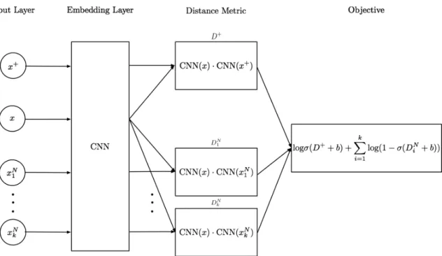
ℒ = ∑︁ (𝑥,𝑙)∈𝐶 (log 𝑝(𝐶 = 1|𝑙, 𝑥+) + 𝑘 ∑︁ 𝑖=0; 𝑥𝑁_∼𝑞 log 𝑝(𝐶 = 0|𝑙, 𝑥𝑁)) (2.2) Here, 𝑘 is the number of samples from the noise distribution. Letting 𝑃 (𝐶 = 1) = 𝜎(𝐷+) and 𝑃 (𝐶 = 0) = 𝜎(𝐷_𝑖𝑁) where 𝐷 is the cosine similarity between the samples, we get the formulation of the objective function in Figure 2-2. We add a bias term 𝑏 to the distance function so that our network can translate the distance to probability easier. Looking at the objective function, the first term brings reads with the same label together. The second term allows the network to learn to push

(21)

Figure 2-2: Noise contrastive estimation takes 2 + 𝑘 input reads with 𝑥+ and 𝑥 having the same label and 𝑥−_𝑖 being sampled from the noise distribution. The reads are mapped to an 𝑛-dimensional space with the same CNN (Net). The dot product between the embeding of 𝑥 and the other reads. These distances 𝐷 are converted to probabilities and the log likelihood is calculated as the objective.

away embedded samples indiscriminately. These two forces allow the network to form clusters of samples with the same labels.

This network is well suited for conserved regions across genomes. If there are regions of DNA that are found across many genomes, reads from these regions will be sampled many times from the noise distribution. By maximizing the distance between these embedded reads and all other embeddings, we expect these embeddings to be reduced to zero magnitude. In this way, non-informative reads can be quickly separated by looking at its magnitude.

(22)

(23)

Chapter 3 Methods for Model Generation and

Analysis

3.1 Data

In our study, we use two datasets: a simulated metagenomic dataset for training and selecting our model and a WMS sequencing dataset to test how well our model does on real data.

We use NCBI’s microbial genome database as our reference genome dataset [3]. This dataset serves as the basis for training and measuring the success of our models against each other. The dataset contains 2860 complete genomes from 739 genus of bacteria. In this reference set, the average length of a genome is 2.2M base pairs. To train our networks we sampled 200bp reads from our reference genomes. 200bps is approximately the length of Illumina’s shotgun sequencing reads. Each base pair in our dataset is one of five labels: A, C, T, G or N (unknown). The taxonomic labels we indirectly used to train our models are based on the genus of the bacteria. For selecting our model we made our training, testing and validation split 70%, 15% and 15% respectively of the reference genome set. We split based on number of genus so that none of the datasets would have overlapping taxonomic labels. We did this so we could test the embeddings of never before seen bacteria.

(24)

of known microbe DNA. This public dataset was generated for analyzing the taxon-omy dependent tool Braken [17]. This dataset contains shotgun sequencing reads from a purified DNA mixture of nine isolate skin bacteria: Acinetobacter radioresistens, Corynebacterium amycolatum, Micrococcus luteus, Rhodococcus erythropolis, Staphy-lococcus capitis, StaphyStaphy-lococcus epidermidis, StaphyStaphy-lococcus hominis, StaphyStaphy-lococcus warneri, and Propionibacterium acnes (NCBI Bioproject PRJNA316735). DNA was extracted and purified from each species. The genomic DNA was mixed together in equal amounts by mass. The DNA mixture was sequenced using Illumina HiSeq to yield 78,439,985 read pairs of length 200bp per spot. Since we know the amount of DNA used in the sample, we can know the exact taxonomic composition.

3.2 Models

To generate the metagenomic read embeddings we train both the triplet network and noise contrastive estimation.

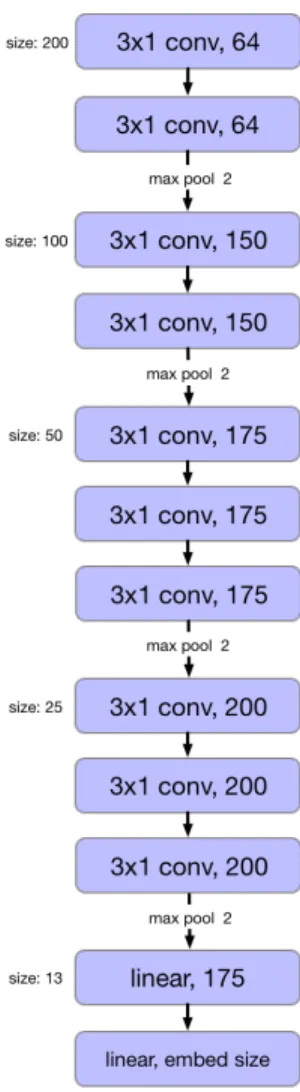
The CNN we use to embed the reads is similar the VGG network [26]. Our CNN contains 10 convolutional filters of size 3x1 each of which is followed by a ReLU and batch norm. By using many small convolutional filters we can get a large receptive field with fewer parameters to train. We summarize the model in Figure 3-1. The final layer of this network determines our embedding size. We try embedding size of 200, 400, and 800 for both the triplet and NCE models. While training the network we sample 1M pairs or triplets from the training set per epoch. We divide the number of sampled reads equally between all genus. Within each genus we divide the samples equally between all genomes.

For for each batch of the triplet network, we have 𝑏𝑎𝑡𝑐ℎ𝑠𝑖𝑧𝑒 triplets (two reads with the same genus and one with a different genus). For each batch of the NCE model, we have 𝑏𝑎𝑡𝑐ℎ𝑠𝑖𝑧𝑒 number of pairs of samples with the same genus and k noise samples from random genus. We share these k noise samples across the batch to make the sampling and computation faster. After embedding the noise samples and the original sample 𝑥, we compute the dot product distance between these samples

(25)

by expanding the first dimension to 𝑏𝑎𝑡𝑐ℎ𝑠𝑖𝑧𝑒. Therefore, the number of reads we sample for each batch is 𝑏𝑎𝑡𝑐ℎ𝑠𝑖𝑧𝑒 * 3 for the triplet network and 𝑏𝑎𝑡𝑐ℎ𝑠𝑖𝑧𝑒 * 2 + 𝑘 for the NCE model. We sample reads uniformly at random from any point in any of the genomes for that taxonomic category.

We train each variation of the model and use validation classification accuracies to select the best model. This validation accuracy determines how well a logistic regression classifier can classify embedded reads from the validation set. To accom-plish this, we split the validation set in half making sure that both sets have at least one genome from each genus. We sample 250,000 reads from each of the validation set splits. We embed these reads using our CNN without the distance or objective function. We train the logistic regression on the first half of these embeddings by including the actual taxonomic class of the embedding. We use the other half to get an accuracy of how well we can predict the labels from this embeddings. The model with the best classification accuracy is chosen as the CNN for our clustering analysis. We also generate a k-mer embedding baseline to compare our accuracy to. We get this baseline by repeating the previous process on the validation set using a k-mer embedding instead.

3.3 Synthetic Clustering

After selecting the best CNN embedding model, we test how well our model can separate reads from novel genus. From our testing dataset, we generate 1000 reads sampled equally across each genus. We embed the reads using k-mer and CNN em-bedding. We perform principal component analysis (PCA) on these embeddings and plot the first two principal components. We cluster these embeddings in this new space using a Bayesian Gaussian mixture model with a Dirichlet process prior. By modeling this using a Dirchlet process prior, we estimate both the number of clusters and the parameters of these clusters (mean and covariance). We compare the true taxonomic label distribution within each cluster to determine how well the model is able to cluster on these embeddings.

(26)

Figure 3-1: Architecture of the CNN encoder. Each convolutional layer is followed by a batch norm and ReLU layer. The convolutional layers are also padded so that the input size does not change.

(27)

3.4 WMS Clustering

To test how well our model can predict the composition of a population, we form clusters from the skin microbiome dataset. We use the same process to generate clusters as the in silico dataset. Here, we use the paired-end reads in each spot of the sequencing data as one read into our model. Although the paired-end reads are not whole, they come from the same region of the same organism. This assumption allows us to work with 200bp reads.

We assign the true taxonomic labels to these reads by generating a BLAST database from genomes of the original nine species of skin microbes. We do a lo-cal BLAST against this database to label these sequencing reads. We measure the success of our tool from how many clusters we get and from how homogeneous these clusters are.

3.5 Implementation Details

After designing the network and analysis, we constructed both networks in Python using PyTorch [22]. Our 𝑏𝑎𝑡𝑐ℎ𝑠𝑖𝑧𝑒 for training the model was 32. We used Adam optimizer with a learning rate of 0.0001 to train our models. We also used k=100 negative samples for NCE where the samples were shared across the batch. All experiments were run using NVIDIA Tesla-K40c GPUs. We ran each model for 50 epochs or until they converged which took about 30 hours. In implementing the validation classifier and the Gaussian mixture model we used the scikit-learn library [23]. The Bayesian Gaussian mixture model had a weight concentration prior 𝛼 = 1𝑒 − 3 and number of components (max number of clusters) of 30.

(28)

(29)

Chapter 4 Results and Discussion

4.1 Results

4.1.1 Modeling

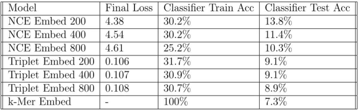
After running the models for 50 epochs, or until it converged, we obtained the loss, classification training and testing accuracies as summarized in Table: 4.1.

The second column shows the final loss for the NCE and Triplet embedding mod-els. Although we cannot directly compare these values, we can see that the Triplet network’s loss varied less with embedding size. This trend can also be seen in the classifier test accuracy. The classification accuracy of the noise-contrastive estimation model had a larger variation in test accuracy. Comparing the classifier test accuracy

Table 4.1: Modeling Results

Model Final Loss Classifier Train Acc Classifier Test Acc

NCE Embed 200 4.38 30.2% 13.8% NCE Embed 400 4.54 30.2% 11.4% NCE Embed 800 4.61 25.2% 10.3% Triplet Embed 200 0.106 31.7% 9.1% Triplet Embed 400 0.107 30.9% 9.1% Triplet Embed 800 0.108 30.7% 8.9% k-Mer Embed - 100% 7.3%

(30)

between the NCE and Triplet network models we notice that all the NCE models out-performed the Triplet models. We hypothesize that because the Triplet model was enforcing a strict comparison between read embeddings with the same label and those with different labels, conserved regions of DNA skewed the model. It seems that the Triplet network has difficulty with samples that appear in multiple contexts. NCE, on the other hand, can deal with these conserved regions by minimizing the magnitude of these embeddings. The NCE model with embedding size of 200 performed the best and was used as our model for the rest of our analysis.

The classifier train accuracy for each of the models was at or around 30% whereas the training accuracy of the k-mer embedding was 100%. The low training accuracy indicates that the embeddings were not completely separable. This suggests that the model has room for improvement. However, it is also important to note that both models had classifier test accuracies that were significantly better than k-mer embed-ding. For classifying reads from novel genus, its better to use a CNN embedembed-ding.

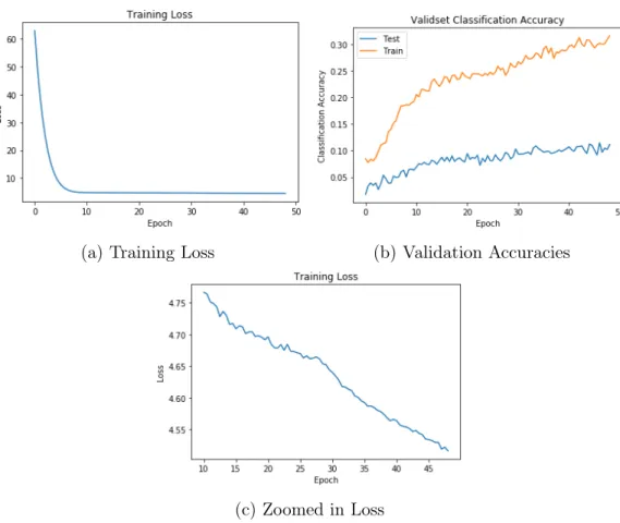
We now look at the training results of our best model (Figure 4-1). These results show that the model converged as the classification test accuracy has stopped in-creasing (Figure 4-1b). Although the training loss seems to have reached a minimum after 10 epochs (Figure 4-1a), on closer inspection we can see that the loss was still decreasing slowly (Figure 4-1c). We hypothesize that the initial decrease in the loss is from tuning our bias term in NCE (Figure 2-2). We initialized this to be zero. We noticed that small changes in this value changed the starting loss dramatically and in some cases caused the model to not converge.

4.1.2 Clustering on Synthetic Data

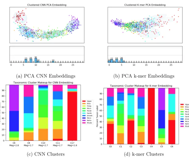
After sampling and embedding reads using k-mer embedding and CNN embedding, we transformed each embedding space using PCA. We generated a graph of the embedded reads over the first two principle components (Figure 4-2a and 4-2b). These plots show each embedded read and its corresponding taxonomic label (one of 10 colors). The overlaid ovals are each cluster from the Bayesian Gaussian mixture model and below it are the percentage breakdowns of the number of read embeddings in each cluster.

(31)

(a) Training Loss (b) Validation Accuracies

(c) Zoomed in Loss

(32)

The CNN embedding has separated some reads with different labels in the taxonomic space. In Figure 4-2a the embedded reads with the red label has been almost entirely separated from the other reads. We see that the CNN is generating an embedding space where reads are clustered by taxa.

This separation can also be seen in the cluster distribution (Figure 4-2c and 4-2d). The red labeled reads are distributed across many clusters in the k-mer embedding space. In the CNN embedding space, almost all of these reads are in one cluster. We can say a similar thing about cluster 10 in the CNN clustering. This cluster captures much of the green labeled read embeddings. Figure 4-2c also presents the the average magnitude of the read embeddings for each cluster. The magnitude of the read embeddings for the less structured clusters (C8, C10, C11) were lower than the magnitudes of the more structured clusters (C6 and C17). This data supports our original hypothesis that reads that are similar to many other reads (close in taxonomic space) would be pushed closer to zero magnitude by our NCE model than those that are more unique to a genus.

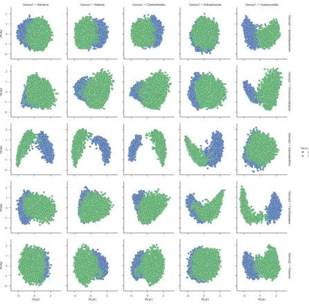
We plotted pairwise comparision of 10 genus in our test set (Figure 4-3). For each square in this 5x5 grid we showed all of the embeddings from two genus in our test set. This allowed us to characterize when read embeddings were separable. Figure 4-3a is colored based on the taxonomic label where each column has the same taxonomic label for the blue embedded reads and each row has the same taxonomic label for the green embedded read. To understand the effect of base pair composition on embedding separation we plotted adenine composition for the same embedded reads (Figure 4-3b). Generally, many of the pairwise comparisons had some separation between the embeddings with the middle row and the rightmost column having the best. 4-3b shows that nucleotide composition is important for good separation of reads.

4.1.3 Clustering on Real Metagenomic Data

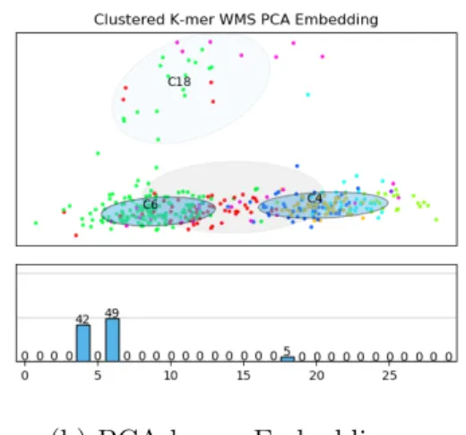
We performed the same clustering techniques on a section of the skin microbiome dataset. In Figure 4-4 we see the clustering results of 400 embedded reads from this

(33)

(a) PCA CNN Embeddings (b) PCA k-mer Embeddings

(c) CNN Clusters (d) k-mer Clusters

(34)

(a) Pairwise comparison of embeddings for 10 genus

(b) Adenine composition for each read in pairwise comparison.

(35)

dataset. We see similar patterns on this dataset as we did on the synthetic dataset. The CNN and k-mer read embedding space are closely related. However, as the clustering shows, the CNN has separated some of these embeddings (Figure 4-4a and 4-4b). The label breakdown of the clusters also shows this trend with C7 and C11 in the CNN Clusters being almost entirely Micrococcus and Staphylococcus respectively. The k-mer clusters do not show this separation as most of the reads are clustered into two large clusters.

(a) PCA CNN Embeddings (b) PCA k-mer Embeddings

(c) CNN Clusters (d) k-mer Clusters

Figure 4-4: Embedding space and cluster breakdown for CNN and k-mer embeddings on WMS dataset.

We analyzed the runtime of each algorithm in our embedding scheme and com-pared it to the runtime of the local BLAST algorithm we used (Table 4.2). Although CNN embedding is not as fast as k-mer Embedding, it is much faster than the local BLAST algorithm we used to generate the labels for the WMS data. This shows that

(36)

Table 4.2: Runtime of Embedding Algorithms per Million Reads

Model Local BLAST CNN Embed 4-mer Embed

Runtime (sec/million reads) 5350 24.0 4.88

CNN embedding is a viable option for processing WMS data.

4.2 Discussion

In this thesis we proposed and analyzed a novel method for taxonomy independent metagenomic binning. We used common tools from NLP and image recognition prob-lems to create a CNN embedding model. The model that preformed the best used noise-contrastive estimation and cosine similarity as the distance function between embeddings. We were able to show that this CNN could be useful for embedding reads into a taxonomically informative space. By training this CNN, we were able generate read embeddings that could be classified better than k-mer embeddings on never before seen organisms. Using a Gaussian mixture model with a Dirichlet pro-cess, we were able to show that our model’s read embeddings were clustered better than k-mer embeddings. On top of our clustering results, our runtime analysis showed that this tool is viable for large scale analysis of WMS data.

One future expansions to this project is more rigorous hyperparameter testing of the models. In particular, varying the model complexity might increase the accuracy of our model. We believe that the model could perform better as our classifier was unable to separate a significant number of read embeddings. We also need to explore why the smaller embedding models performed better on the classification task even though the space of taxonomic labels is much larger than the embedding size. Higher dimensional embeddings should be easier to separate by a classifier, however the training accuracy for our classifier remained mostly the same across embedding sizes. Despite this, our tool has a number of uses. We can use this model to embed reads from a gene of interest. Based on where these genes land, we could identify

(37)

similar organisms with this gene or gene variants that are important in to that class of organisms. The model can also be used to cluster metagenomic reads so that other pipelines can align these reads and reconstruct genomes of bacteria.

(38)

(39)

Bibliography

[1] Stephen Altschul. Basic local alignment search tool (blast). 215:403–410, 10 1990.

[2] Yasir Bashir, Salam Singh, and Bolin Konwar. Review article metagenomics: An application based perspective. 2014:1–7, 08 2014.

[3] Dennis A. Benson, Mark Cavanaugh, Karen Clark, Ilene Karsch-Mizrachi, David J. Lipman, James Ostell, and Eric W. Sayers. Genbank. Nucleic Acids Research, 41(D1):D36–D42, 2013.

[4] Marilia Carabotti, Annunziata Scirocco, Maria Antonietta Maselli, and Carola Severi. The gut-brain axis: Interactions between enteric microbiota, central and enteric nervous systems. 28:203–209, 04 2015.

[5] Sourav Chatterji, Ichitaro Yamazaki, Zhaojun Bai, and Jonathan A. Eisen. Com-postbin: A dna composition-based algorithm for binning environmental shotgun reads. In Martin Vingron and Limsoon Wong, editors, Research in Computa-tional Molecular Biology, pages 17–28, Berlin, Heidelberg, 2008. Springer Berlin Heidelberg.

[6] Kevin Chen and Lior Pachter. Bioinformatics for whole-genome shotgun se-quencing of microbial communities. PLoS Computational Biology, 1(2):e24, 07 2005.

[7] Chris Dyer. Notes on noise contrastive estimation and negative sampling. CoRR, abs/1410.8251, 2014.

[8] Kei Fujimura, Alexandra Sitarik, Suzanne Havstad, Din L Lin, Sophia Levan, Douglas Fadrosh, Ariane Panzer, Brandon LaMere, Elze Rackaityte, Nicholas W Lukacs, Ganesa Wegienka, Homer A Boushey, Dennis Ownby, Edward M Zo-ratti, Albert M Levin, Christine Johnson, and Susan Lynch. Neonatal gut micro-biota associates with childhood multisensitized atopy and t cell differentiation. 22, 09 2016.

[9] Ivan Gregor, Johannes Drage, Melanie Schirmer, Christopher Quince, and Alice C. McHardy. Phylopythias+: A self-training method for the rapid reconstruction of low-ranking taxonomic bins from metagenomes. 4, 06 2014.

(40)

[10] Elad Hoffer and Nir Ailon. Deep metric learning using triplet network. CoRR, abs/1412.6622, 2014.

[11] Gregory Koch, Richard Zemel, and Ruslan Salakhutdinov. Siamese neural net-works for one-shot image recognition. 2015.

[12] Anna Kopf, Elmar Pruesse, Timmy Schweer, JÃČÂűrg Peplies, Christian Quast, Matthias Horn, and Frank Glackner. Evaluation of general 16s ribosomal rna gene pcr primers for classical and next-generation sequencing-based diversity studies. 41, 08 2012.

[13] Victor Kunin, Alex Copeland, Alla Lapidus, Konstantinos Mavrommatis, and Hugenholtz Philip. A bioinformatician’s guide to metagenomics. 72:557–78, Table of Contents, 01 2009.

[14] Cedric C. Laczny, Tomasz Sternal, Valentin Plugaru, Piotr Gawron, Arash Atashpendar, Houry Hera Margossian, Sergio Coronado, Laurens van der Maaten, Nikos Vlassis, and Paul Wilmes. Vizbin - an application for reference-independent visualization and human-augmented binning of metagenomic data. Microbiome, 3(1):1, Jan 2015.

[15] Ben Langmead, Cole Trapnell, Mihai Pop, and Steven Salzberg. Langmead b, trapnell c, pop m, salzberg sl.. ultrafast and memory-efficient alignment of short dna sequences to the human genome. genome biol 10: R25. 10:R25, 04 2009. [16] Heng Li and Richard Durbin. Fast and accurate long-read alignment with

burrows-wheeler transform. 26:589–95, 03 2010.

[17] Jennifer Lu, Florian P. Breitwieser, Peter Thielen, and Steven L. Salzberg. Bracken: estimating species abundance in metagenomics data. PeerJ Computer Science, 3:e104, January 2017.

[18] Yunan Luo, Y. William Yu, Jianyang Zeng, Bonnie Berger, and Jian Peng. Metagenomic binning through low density hashing. bioRxiv, 2017.

[19] Tomas Mikolov, Kai Chen, Greg Corrado, and Jeffrey Dean. Efficient estimation of word representations in vector space. CoRR, abs/1301.3781, 2013.

[20] Andriy Mnih and Yee Whye Teh. A fast and simple algorithm for training neural probabilistic language models. 2, 06 2012.

[21] Rachid Ounit, Steve Wanamaker, Timothy Close, and Stefano Lonardi. Clark: Fast and accurate classification of metagenomic and genomic sequences using discriminative k-mers. 16, 03 2015.

[22] Adam Paszke, Sam Gross, Soumith Chintala, Gregory Chanan, Edward Yang, Zachary DeVito, Zeming Lin, Alban Desmaison, Luca Antiga, and Adam Lerer. Automatic differentiation in pytorch. 2017.

(41)

[23] F. Pedregosa, G. Varoquaux, A. Gramfort, V. Michel, B. Thirion, O. Grisel, M. Blondel, P. Prettenhofer, R. Weiss, V. Dubourg, J. Vanderplas, A. Passos, D. Cournapeau, M. Brucher, M. Perrot, and E. Duchesnay. Scikit-learn: Machine learning in Python. Journal of Machine Learning Research, 12:2825–2830, 2011. [24] Marta Pozuelo, Suchita Panda, Alba Santiago, Sara Mendez, Javier Santos, and Francisco Guarner. Reduction of butyrate- and methane-producing microorgan-isms in patients with irritable bowel syndrome. Scientific Reports, 5, 2015. [25] Karel Sedlar, Kristyna Kupkova, and Ivo Provaznik. Bioinformatics strategies

for taxonomy independent binning and visualization of sequences in shotgun metagenomics. 15, 12 2016.

[26] Karen Simonyan and Andrew Zisserman. Very deep convolutional networks for large-scale image recognition. CoRR, abs/1409.1556, 2014.

[27] Derrick E. Wood and Steven L. Salzberg. Kraken: ultrafast metagenomic se-quence classification using exact alignments. Genome Biology, 15(3):R46, Mar 2014.

[28] Yu-Wei Wu and Yuzhen Ye. A novel abundance-based algorithm for bin-ning metagenomic sequences using l-tuples. In Bonnie Berger, editor, Research in Computational Molecular Biology, pages 535–549, Berlin, Heidelberg, 2010. Springer Berlin Heidelberg.