A design optimization framework for enhanced compressor stability using dynamic system modeling

A Design Optimization Framework for Enhanced

Compressor Stability Using Dynamic System Modeling

by

Vincent P. Perrot

Submitted to the Department of Aeronautics and Astronautics in partial fulfillment of the requirements for the degree of

MASTER OF SCIENCE IN AERONAUTICS AND ASTRONAUTICS

MASSACHUSETTS INSTITUTE OF TECHNOLOGY

September 2003

@Vincent P. Perrot 2003. All rights reserved.

The author hereby grants to MIT permission to reproduce and distribute publicly paper and electronic copies of this thesis document in whole or in part, and to grant others the right to do so.

Author - ,

Departme I+-on6ri s and Astronautics August 22, 2003

Certified by

Accepted by

Profissor olt6n S. Spakov ky C.R. Soderberg Assistant Professor of Aeronautics and Astro utics Thesis Stipervisor

I

Profesdor Edward M. Greitzer

H.N. Slater Professor of Aeronautics and Astronautics

MASSACHUSETTS INSTITUTE OF TECHNOLOGY

NOV 0

5

2003

A Design Optimization Framework for Enhanced

Compressor Stability Using Dynamic System Modeling

by

Vincent P. Perrot

Submitted to the Department of Aeronautics and Astronautics on August 22-2003, in partial fulfillment of the

requirements for the degree of

Master of Science in Aeronautics and Astronautics

Abstract

This thesis constitutes the second year effort of a joint engineering project initiated in 2001 by Snecma Moteurs, ENSAE, ECL and MIT. The long term objective of this joint project is to conceive, design, implement and operate an advanced core compressor for an unmanned air vehicle. This thesis addresses the issue of compressor design in the light of enhanced stability, introducing a novel approach with respect to industry-practice: compressor dynamic stability is to be considered as a prime design variable.

This present study focuses on the development and implementation of a compressor design optimization framework for enhanced stability based on an existing reduced order dynamic system modeling approach [15]. Stall margin, a common metric for compressor stability, is chosen as an optimization objective in the light of performance constraints. Modifications of the shape of the blade-row loss buckets are the optimization design variables since they directly impact compressor performance and dynamic stability.

An optimization framework is defined, with the goal to redesign a baseline compressor through geometric modifications, optimized for enhanced stability. The framework is comprised of a mean line calculation including end-wall effects, and the computation of the unsteady flow field perturbations using the existing dynamic compression system model. A solution to the resulting inverse-design problem introduced by the optimization problem is devised. Changes in blade-row loss buckets are linked analytically to a modification of the blade channel angle.

The inverse-design optimization framework is implemented on a 3-repeating-stage compressor leading to a 6.4% improvement of the stall margin while changes in performance are kept to a minimum of 2% loss in pressure ratio and 0.5% loss in efficiency. The definition of a new compressor geometry is obtained from the baseline compressor through the introduction of modifications to the blade channel angles of the blade-rows which range between -0.3' and 2.7.

Thesis Supervisor: Professor Zoltin Spakovszky

Acknowledgements

I first want to thank Professor Spakovszky for all the fruitful discussions that we had over the

year. I am thankful for his support, his always critical look at my work leading to deeper understanding and better outcomes.

I am also grateful to my research partner Josep M. Dorca-Luque for the great moments we spent

working together during which he shared with me his experience in the turbo-machinery world. Beyond work, we developed a real friendship and I must acknowledge that he taught me how to talk to computers in Catalan.

I am indebted to my officemates Chris, David and Mark for teaching me each day new things

about this country and who took a real part in my introduction to the true American Experience. I also want to thank Alexis, my lab mate and social hour co-organizer, for the always enjoyable moments spent talking together.

My last thanks go to Professor Carrere from my engineering school ENSAE in France, for being

one of the instigators of the joint project with MIT and who enabled me to enjoy this wonderful time spent here at the Gas Turbine Lab.

Contents

1.1 Technical Background: Rotating Stall and Surge... 19

1.2 W hy Design for Enhanced Stability?... 23

1.3 The Joint Project ... 23

1.4 Previous W ork and Ongoing Efforts... 25

1.5 Thesis Organization...25

1.6 Objectives ... 26

1.7 Contributions...26

The O ptim ization Loop: M ajor Features... 28

2.1 Overview of the Optim ization Loop ... 29

2.2 M ean-Line Calculation ... 30

2.3 Reduced Order Dynam ic Com pressor M odel ... 31

2.3.1 Underlying Theory ... 31

2.3.2 Eigenvalue Search to Determine the Point of Limit Stability... 33

2.4 End-W all Correlations...36

2.5 Conclusion ... 41

Influence of Blade-Row Losses on Compressor Performance and Stability ... 42

3.1 Com pressors Characteristics From First Principles ... 42

3.2 Demonstration of Blade-Row Contribution to Compressor Dynamics...45

Analytical Dependence of Blade-Row Losses on Blade Geometry ... 51

4.1.2 Thickness M odification...53

4.1.3 Blade Chord Effects on the M inimum Loss Level ... 53

4.1.4 M od ifications to the Blade Channel ... 54

4.2 Practical Implementation of M odifications to the Blade Channel... 54

4.2.1 Geometric Implementation...54

4.2.2 Effect of M odifications to the Blade Channel on Blade-Row Loss: Diffusion Effects...55

4.2.3 Least Squares Interpolation Between Losses, Incidence and Abc ... 57

4.2.4 Example of Implementation of the Least Squares Interpolation... 58

4.2.5 Another Possible M ethod to Interpolate the Computed Losses ... 61

4.3 Conclusion ... 62

Assessment of Effects of Blade Channel Modifications on Compressor Performance and Stability ... 64

5.1 Analysis of the Sensitivity of Compressor Performance and Stability to Blade Channel M odifications -Profile Loss Only ... 64

5.1.1

Qualitative

5.1.2 Quantitative Analysis ... 67

5.1.3 C on clusion s...69

5.2 Analysis of the Sensitivity of Compressor Performance and Stability to Blade Channel M odifications -Profile and End-W all Loss ... 69

5 .3 C on clu sion ... 72

Preliminary Design Optimization of a 3-Stage Repeating Stage Compressor for Enhanced Stability ... 73

6.1 Presentation of the Objectives and Design Variables of the Optimization ... 73

6.2 Optimization Details...74

6.2.1 A lg orithm s ... 75

6.2.2 M ulti-Objective Problem: Weighted Sum Approach...77

6.3 Proof of Concept: Results and Discussion... 78

6.3.1 Formal Formulation of the Problem... 78

6.3.2 Algorithm Settings ... 80

6.3.3 Optimization Results ... 80

6.3.4 Parametric Study on the Weights Used in the Objective Function... 85

C onclusions and Future W ork ... 87

7.1 Sum m ary and Conclusions...87

7.2 Future W ork...88

A ppendix A...90

A ppendix B...93

List of Figures

Figure 1-1: Pressure ratio - Mass flow characteristic showing the location of the stall point...20

Figure 1-2: Physical mechanism for inception of rotating stall (from [6]) ... 21

Figure 1-3: Schematic presenting the circumferential modes... 22

Figure 1-4: Types of compression system instability (adapted from [7])...22

Figure 1-5: Joint project fram ew ork ... 24

Figure 1-6: Diagram presenting the optimization framework ... 25

Figure 2-1: Optimization loop overview ... 29

Figure 2-2: Single-stage axial compressor model...31

Figure 2-3: Eigenvalues for a 3-stage compressor for a given operating point shown on the corresponding compressor characteristic ... 34

Figure 2-4: Schematic of the search routine to determine the point of limit stability ... 35

Figure 2-5: Definition of the blades staggered spacing (g) ... 37

Figure 2-6: Calculation procedure implementing end-wall effects ... 38

Figure 2-7: Additional stagnation pressure loss due to end-wall effects... 38

Figure 2-8: Loss bucket for rotor 1 of the 3-stage, repeating-stage compressor with and without end-w all correlation s ... 41

Figure 3-1: Howell's breakdown of loss for an axial stage (From Cumpsty [31)... 43

Figure 3-2: Sketch of a compressor characteristic ... 44

Figure 3-3: Blade-row loss buckets of the 3-stage, repeating-stage compressor - baseline and with m od ifications to rotor 1 ... 46

Figure 3-4: Characteristics of the baseline 3-stage compressor and of the compressor with m odifications to rotor 1 ... 47

Figure 3-5: Blade-row loss buckets of the 3-stage, repeating-stage compressor - baseline and with m odifications to rotor 1 ... 48

Figure 3-6: Characteristics of the baseline 3-stage compressor and of the compressor with m odifications to rotor 1 ... 49

Figure 4-1: Influence of airfoil camber line on stagnation pressure loss (adapted from [3])...52

Figure 4-2: Influence of airfoil thickness on stagnation pressure loss (adapted from [3])...53

Figure 4-3: Influence of airfoil chord on stagnation pressure loss...53

Figure 4-4: Illustration of modifications to the blade channel...55

Figure 4-6: Preliminary analysis to determine an analytical relation between 2D blade-row loss and

blade channel geom etry ... 58

Figure 4-7: Loss buckets and their interpolation based on a least squares method ... 59

Figure 4-8: Interpolation of the computed loss data... 60

Figure 4-9: Schematic of a method to describe analytically the computed blade-row losses ... 62

Figure 4-10: Example of implementation of the blade channel / loss relation ... 63

Figure 5-1: Rotor 1, baseline and with a blade channel angle change of Abc = +3", loss bucket as a function of flow coefficient ... 65

Figure 5-2: Loss buckets as the function of flow coefficient for the baseline compressor and modified com p ressor ... 66

Figure 5-3: 3-repeating-stage compressor characteristics -baseline compressor and with a blade channel angle change of Abc = +3o for rotor 1 ... 66

Figure 5-4: Sketch presenting two possible optimization strategies... 71

Figure 5-5: Dependency of the difference between results computed with and without end-wall effects on the angle of blade channel modification Ab...72

Figure 6-1: Sketch presenting the iterative process for a gradient-based algorithm (adapted from [171) ... 7 6 Figure 6-2: Blade-row loss of the baseline and optimized compressors ... 83

Figure 6-3: Compressors characteristic of the baseline and optimized configurations...84

Figure 6-4: Blade passage geometries before and after the optimization ... 84

Figure A-1: Definition of the angles and notations used in the mean line calculation ... 90

Figure A-2: Sketch presenting the gaps numbering used in the mean line calculation as well as the d u ct geom etry ... 93

List of Tables

Table 2-1: Comparison of the 3-stage repeating-stage compressor performance with and without

end-w all effects ... 40

Table 3-1: Comparison of performance and stability between baseline and modified configuration ...47

Table 3-2: Comparison of performance and stability between baseline and modified configuration ...49

T able 4-1: B lade geom etry ... 56

Table 4-2: Blade DF, turning and area ratio at 1.60 incidence ... 57

Table 4-3: Comparison between computed and interpolated data for the three loss buckets shown in F ig u re 4 -7 ... 59

Table 4-4: Comparison between computed and interpolated data for the three loss buckets ... 61

Table 5-1: Sensitivity analysis of rotor 1 modification... 67

Table 5-2: Effects of rotor 1 blade channel modifications on the diffusion factor of the blade-rows...67

Table 5-3: Sensitivity analysis of stator 1 modification ... 68

Table 5-4: Effects of stator 1 blade channel modifications on blade-row diffusion factor... 68

Table 5-5: Sensitivity analysis of compressor-wide modifications ... 68

Table 5-6: Impact of modifications of the blade channel angle of rotor 1 on performance and stability ... 7 0 Table 5-7 Impact of modifications of the blade channel angle of stator 1 on performance and stability ... 7 0 Table 5-8: Impact of compressor-wide modifications of blade channel angles on performance and stab ility ... 70

Table 6-1: Results of the optimization calculations... 81

Table 6-2: Blade channel modifications for the optimized compressor's blade-rows ... 82

Table 6-3: Diffusion factors and turning of the baseline and the optimized compressor...82

Table 6-4: Summary of the optimized compressor's performance and stability (compared to the baselin e com p ressor)...82

Table 6-5: Results of optimizations carried out on objective functions with different weight d istrib u tion s...85

Table B-1: Duct geometry of the 3-repeating-stage compressor ... 93

Table B-2: Blades geometry of the 3-repeating-stage compressor ... 93

Nomenclature

B transmission matrix

c polynomial interpolation coefficients

CFD Computational Fluid Dynamics

DF Diffusion Factor

EC exit conditions

ECL Ecole Centrale Lyon

ENSAE Ecole Nationale Sup6rieure de lAronautique et de l'Espace

f function linking blade-row loss and geometry

g blade staggered spacing

g inequality constraint GA Genetic Algorithm h equality constraint i incidence, index IC initial conditions j j = V1

J

L blade-row loss coefficient

m correlation coefficient

M Mach number

fiz mass flow

n correlation coefficient, harmonic number

OPR Overall Pressure Ratio

P pressure Pt total pressure R stage reaction Re Reynolds number s Laplace variable S search direction SM Stall Margin

T transmission matrix

U mean wheel speed

V tangential velocity

V non dimensional absolute velocity, relative velocity

x design vector

X transmission matrix

Y transmission matrix

greek

a absolute flow angle, distance from previous point

p

6* end-wall axial-velocity boudary layer displacement thickness

A difference (when used as a prefix)

Abc _{blade channel angle modification}

flow coefficient

y blade stagger angle

11 adiabatic efficiency

X blade-row inertia, interpolation coefficient, Lagrange multiplier, objective weight

pt stator blade-row inertia

4

p fluid density

a growth rate / rotor frequency

T time lag

) end-wall tangential-force boundary layer thickness

'T pressure rise

o0 blade-row loss coefficient

o0 rotation rate / rotor frequency

subscripts

1 inlet or upstream

2 outlet or downstream

ax axial

design at design point

gap inter-blade-row gap

peak at the peak R rotor ref reference rot rotor s stator sta stator

stan at stall point

Sys system 0 circumferential direction tip x cartesian coordinate cartesian coordinate supercripts is _isentropic ts _{total-to-static}

Chapter 1

Introduction

Currently, a number of research efforts focus on the optimization of the geometry of compressor blade-rows. For instance, Buche et al. [21 focus on the optimization of single subsonic compressor rows for aerodynamic performance (operating range and loss level) and mechanical integrity. As reflected in [2], the industry-practice main objective for compressor optimization is aerodynamic performance. In industry, compressors are designed for enhanced performance while stability requirements are introduced as constraints, but not prime design variables. This research features a new approach: a compressor design optimization framework for enhanced stability is established, based on dynamic compression system modeling. The overall stability of a compressor, in the light of its performance, is to be optimized. The inclusion of stability as a new design objective re-shapes the design space boundaries and thus opens regions never explored before, leading to new possibilities and enabling more aggressive designs. Such an approach could help engine manufacturers develop more robust engines (i.e. more resistant to transient operation, inlet distortion, icing, engine deterioration, etc.) at low cost, since stability problems encountered, once the engine is designed, can lead to costly modifications. These costly modifications could be avoided by design optimizations for enhanced stability.

This chapter first outlines some theoretical principles regarding rotating stall and surge mechanisms, then presents the motivations of this thesis with the objectives and contributions.

1.1

Technical Background: Rotating Stall and Surge

Rotating stall and surge in axial compressors have been the subject of numerous academic theses, research articles or technical books for many years. This indicates the importance attached to the understanding of the physical mechanisms leading to rotating stall and surge in order to prevent them from occurring in-flight. It is hence useful to review succinctly the stall and surge inception

Rotating stall is a localized phenomenon in which regions of stalled flow (referred to as stall cells) appear over a sector of the circumference of a compressor. This is basically a way for the compressor to adapt to small mass flows. Some regions contain locally high mass flows. Others contain almost no flow at all: these are the stalled regions. These regions of stalled flow travel circumferentially at a fraction of the compressor rotation rate, at frequencies between 20-50 % of rotation speed.

Surge is, on the other hand, a compression-system instability. The annulus averaged mass flow and the system pressure rise during surge undergo large amplitude oscillations. The frequencies of these oscillations are generally at least one order of magnitude below those associated with passage of a rotating stall cell and depend on the parameters of the entire system. In addition, during the surge cycles, the instantaneous mass flow through the compressor changes from values at which (in steady operation) the compressor would be free from stall, to values at which one would find rotating stall or totally reversed flow.

Both of these phenomena (surge and rotating stall) are seen to be quite distinct. However, they are not unrelated, since often the occurrence of the local instability (associated with the onset of rotating stall) can trigger the more global type of instability (leading to surge). Reducing the mass flow from the operating point, a maximum pressure ratio is achieved as shown in Figure 1-1. Beyond this point, the compressor enters into either stall or surge. The point of occurrence of this phenomenon is referred to as the stall point.

Stall point 0

Mass fio reduction

Operating point

msurge _{Mass flow}

Figure 1-1: Pressure ratio - Mass flow characteristic showing the

location of the stall point.

Stall Inception Mechanisms

The basic explanation of the mechanism associated with the onset of stall propagation can be summarized as follows (described by Greitzer in [6]). Consider a row of axial compressor blades operating at a high angle of attack, such as shown in Figure 1-2. Suppose that there is a nonuniformity in the inlet flow such that a locally higher angle of attack is established near blade B which is enough

to stall it. If this happens, the flow can separate from the suction surface of the blade so that a substantial flow blockage occurs in the channel between B and C. This blockage causes a diversion of the inlet flow away from blade B and towards C and A (as shown by the arrows), resulting in an increased angle of attack on blade C and a reduced angle of attack on blade A. Since C was on the verge of stall before, it will now tend to stall, whereas the reduced angle of attack on A will inhibit its tendencies to stall. The stall will thus propagate along the blade-row in the direction shown, and under suitable conditions it can grow to a fully developed cell covering half the flow annulus or more. When covering a wide circumferential sector of the annulus and extending over the full length of the machine, the flow disturbances are referred to as modal oscillations. The term "modal" defines circumferential modes, the first mode having a wavelength equal to the circumference, the second

twice its circumference, etc. (see Figure 1-3).

C -7 ; 47 B Direction of stall propagation A Compressor blade-row

Figure 1-2: Physical mechanism for inception of rotating stall (from [61).

It has to be kept in mind that rotating stall and surge are the mature forms of small amplitude flow perturbations that are the natural resonances of oscillations in the compression system, these small disturbances grow when background flow conditions are such that their damping becomes negative and the compression system drops into an unstable state, rotating stall or surge.

Spakovszky (see [15] and [16]) developed an analytical, dynamic compression system model aimed at the determination of the fundamental flow resonances (circumferential modes or eigenvalues of the unsteady flow field) in axial and radial compressors. Spakovszky's dynamic compression system model is the central part of this thesis, and is used to predict the stability of axial compressors. The model will be presented with more detail in Chapter 2.

LII~

Front view of an axial compressor duct

0

Mode 1

oode22

Stability Analysis of a Compression System

Two criteria have to be met for a compression system to be stable: static stability and dynamic stability. Static instability (illustrated on the left of Figure 1-4) is associated with a pure divergence from initial state (analogous to a mechanical system with negative spring constant) and is related to the slopes of the throttle line and the compressor characteristic. For a small perturbation in mass flow (a decrease, say), if the system is operating at point A, a pressure imbalance will arise to cause fluid accelerations that return the system to operation at the initial point. Point A is thus a stable operating point. At point B, however, where the throttle line is tangent to the compressor characteristic, the pressure forces associated with a small decrease in mass flow will cause the system to depart further from the initial operating point, so that point B is an unstable operating point.

STATIC INSTABILITY DYNAMIC INSTABILITY

B AD B

4Compressor

Throttle lines Throttle line

Mass flow Mass flow

UNSTABLE IF SLOPE OF COMPRESSOR EVEN IF STATICALLY STABLE, SYSTEM

CHARACTERISTIC GREATER THAN SLOPE CAN BE DYNAMICALLY UNSTABLE

OF THROTTLE LINE (POINT B) (POINT D)

This first criterion is, however, too simple to describe the real phenomenon, since it only considers the static stability of the system. In fact, it is generally the dynamic stability criteria which are violated first, leading to growing oscillatory motion. As indicated on the right side of Figure 1-4, a compression system can be statically stable (according to the foregoing slope criterion) and still exhibit instability. In summary, static stability is necessary for a compression system to be stable but is not sufficient.

The static and dynamic stability behavior of compression systems is captured by Spakovszky's dynamic model.

1.2

Why Design for Enhanced Stability?

Why should stability be taken into account at the early stage of compressor design?

Blanvillain [1] assessed how much an in-flight surge event potentially costs an airline operating such an aircraft. This type of problem is a very unwanted event because it can cost the airline up to

$3.5 million. Furthermore, running a fleet of reduced-stability engines can cost a major airline up to $10 million a year. These expenses can represent up to 8% of the total revenue potentially generated by the fleet powered by these engines. The probability of in-flight surge could be reduced and engine

stability enhanced if stability was taken into account from the early stage of design.

Furthermore, to limit potential risks associated with surge events, industry design practice and certification authorities impose a substantial margin, called stall margin (or surge margin), intended to keep the engine operating away from the stall boundary. Several uncertainties are associated with stall margin, such as inlet distortion, transient operation, icing or engine deterioration. All these uncertainties are built into stall margin that is consequently increased, leading to a reduction in blade loading and diffusion, entailing sub-optimal designs as operating conditions are typically moved away from points of high efficiency. The key idea of this research is to incorporate dynamic stability as a prime design objective and to establish a compressor design framework optimizing for enhanced stability.

First, the background and motivation for this thesis are introduced followed by the presentation of a joint project in which this research is embedded.

1.3

The Joint Project

This thesis is part of a joint project initiated in 2001 by Snecma Moteurs, the Ecole Nationale Sup6rieure de l'Aronautique et de l'Espace (ENSAE), the Ecole Centrale de Lyon (ECL) and the

them an opportunity to work in an international environment on complex systems and to develop their skills in the gas turbine engine field. A detailed description of the respective contributions of the parties involved is reviewed in Blanvillain [1].

MIT's part of the project focuses on the inverse-design of an axial compressor using an existing reduced order dynamic compressor model embedded in an optimization framework for performance and stability.

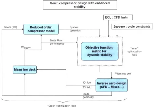
The architecture of this framework is presented in Figure 1-5. From an original aerodynamic design, performance characteristics of a compressor can be obtained and its dynamic behavior can be evaluated using the reduced order model. Once the dynamics of the modal oscillations are determined, a metric is involved to assess the dynamic stability of the system. The shape of the loss buckets can then be altered in an inner optimization loop in order to increase the level of stability to pre-defined objectives. The shapes of the loss buckets are chosen to be the optimization design variables since compressor stability is affected by the loss characteristics. This is because the compression system dynamics consist of pre-stall modes which depend on the background flow field.

Goal compressor design with enhanced

stability

ECL: CFD limits

Geom (2D) Reduced order System Supaero cycle constraints

compressor model dynamics

Blade Row performance

loss - -ObjeCtive fUNction: *1nner"

metric fOr optimization

dynmiC stability loop

Moan line dock

loss opt. perf

3D flow Ines w slg 2D field (CFD -Mss.)

Blade geometry

"Outer" optimization loop

Figure 1-5: Joint project framework.

The last task is the definition of the geometric modifications leading to the prescribed loss buckets. This inverse-design problem can be solved using CFD calculations and a mean line deck. The new geometry obtained from the prescribed loss buckets is then fed into the dynamic calculation and the process is repeated until convergence in performance and stability is achieved.

1.4

Previous Work and Ongoing Efforts

This thesis is the second step of the project. Blanvillain's work represented the first-year effort. He implemented Spakovszky's reduced order model [151 for a multi-stage axial compressor, and carried out a series of parametric studies aimed at defining preliminary compressor design guidelines for enhanced stability.

The project was then divided into two parallel efforts. This thesis focuses on the inverse-design optimization for enhanced stability. A more thorough description of the optimization framework is given in next section. The other effort carried out at the same time by Dorca [4] focuses on an energy-based analysis of compressor stability and is aimed at the development of a metric for stability that could eventually be used as an optimization objective.

1.5

Thesis Organization

The optimization framework developed in this thesis is now presented. It is an implementation of the inverse-design architecture presented in section 1.3, although it differs from it since the inverse design optimization for enhanced stability is solved in a single optimization loop.

j

/

S

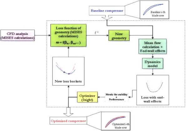
Figure 1-6 depicts the path followed from a given baseline compressor to the eventual optimized compressor for enhanced stability. The main idea as follows: a baseline compressor to be optimized for stability is defined in terms of its geometry and individual blade-row losses. The performance of the baseline compressor is computed using a mean line calculation including end-wall effects and the eigenvalues for modal flow oscillations are found using Spakovszky's model (performance and dynamic calculations are described in Chapter 2). From the aforementioned calculations, the level of performance and stability of the baseline compressor are measured.

The loss buckets of the blade-rows are then modified by using the commercially available optimizer Isight, with the objective of achieving a prescribed level of stability in the light of performance constraints. The shapes of the blade-row loss buckets prescribed by the optimizer are then linked to geometric modifications inside the optimization loop. The steps (based on a preliminary CFD analysis) leading to the determination of a function f, the solution to the inverse-design problem linking a change in a blade-row loss bucket to a modification of a blade-row geometry, are described in Chapters 3, 4 and 5.

Once the new geometry stemming from the new loss buckets is defined, the calculation is iterated until an optimized solution meeting the stability and performance requirements is found. The optimization process is explained in Chapter 6 leading to the optimization of a 3-stage repeating-stage compressor.

1.6

Objectives

The objectives of this thesis are to:

e Assess and analytically describe the relation between blade-row loss, geometry, performance and stability.

" Identify and implement geometric design variables linked to modifications of the blade-row loss in order to perform a compressor design optimization for enhanced stability.

" Propose a design framework capable of optimizing a compressor for enhanced stability in the light of performance constraints, using an existing dynamic compressor model.

" Demonstrate the framework capabilities by solving an optimization problem for a generic 3-stage, repeating-stage compressor comprised of blade-rows with NACA0012 profiles.

* Devise design implications using the optimization framework.

1.7

Contributions

* Definition of an inverse-design optimization framework for enhanced compressor stability, based on dynamic compression system modeling,

* Feasibility assessment of the compressor design framework optimizing for enhanced stability,

* Implementation and demonstration of this design-framework for a 3-repeating-stage compressor.

Chapter 2

The Optimization Loop: Major

Features

To perform the optimization loop as presented in Figure 1-6 going from a baseline compressor to the optimized one, a simulation code or optimization loop is needed to implement and to combine the mean line calculation, the dynamic model, the loss interpolations and the end-wall correlations. This loop will eventually be closed by the optimizer which enables the iterative optimization process. Without going into the details of the optimization, this chapter focuses on all the components that have to be combined to form the optimization framework. The aim is the following: a compressor geometry is specified, given the losses and deviations corresponding to each blade-row, and the operating conditions (speed, external thermodynamic conditions). From this set of data, one wants to be able to predict:

* the compressor performance (typically overall pressure ratio and overall adiabatic efficiency) computed using a compressible mean flow calculation including end-wall effects and taking into account deviation and loss data. Performance is to be computed at low speed because Mach number effects on the losses and additional shock-induced losses are neglected.

e _{the compressor stability (taking for instance stall margin as a metric for stability)} computed using an incompressible compression system dynamic model.

Keeping these objectives in mind, this chapter first introduces an overview of the different steps encountered in the optimization loop. Next, all the linked modules are presented along with their limitations and the assumptions made.

2.1

Overview of the Optimization Loop

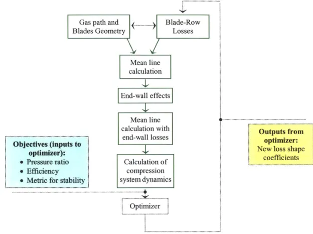
Before describing all the modules, an overview of the framework is given, together with the links between the different components. Figure 2-1 presents a sketch of the loop that is eventually closed

by the optimizer.

... _{n 1 W ll l S e}

-endt-wall tosses Objectives (inputs to

optimizer):

* Pressure ratio Calculation of

* Efficiency compression

e Metric for stability system dynamics Optimizer

Outputs from optimizer. New loss shape

coefficients

... .

Figure 2-1: Overview of the optimization loop.

Conceptually, the aim of the optimization loop is to compute the overall pressure ratio, adiabatic efficiency and stall margin of a given compressor.

The inputs to the calculation are the geometry of the gas path and the blades, as well as the loss descriptions of all the blade-rows. To get the compressor performance, a first mean line calculation using these inputs is performed. From this performance, end-wall correlations are implemented, leading to a re-definition of the blade-row loss, including end-wall effects.

The mean line calculation is then performed for the second time using the loss buckets with end-wall effects as inputs. This mean line calculation also provides the velocity field, flow angles, blade-row loss and loss derivatives, which are necessary inputs to the calculation of the compressor

pre-stall dynamics. This calculation enables the computation of the compressor pre-stall margin which is another objective function in the optimization loop.

Next, more details on the mean line calculation, the dynamic compressor model, and the implementation of end-wall effects are given.

2.2

Mean-Line Calculation

The mean line calculation is used to compute the performance of any given compressor (one is interested in the overall pressure ratio and the overall adiabatic efficiency). For that calculation to be carried out, the following inputs have to be specified:

* number of stages,

* hub and tip radii at mid-axial position between each blade-row, * lengths of the blade-row and inter-stage gaps,

* blade chords,

* inlet and outlet metal angles as well as stagger angles for all blade-rows.

Furthermore, the inlet flow conditions and rotational speed have to be specified: * inlet static pressure and temperature,

* rotation speed, e inlet swirl angle.

Finally, the effects of blade-row loss and deviation (functions of incidence) have to be input.

Using this data, the compressor performance is obtained, that is the overall pressure ratio and the overall adiabatic efficiency maps as functions of corrected mass flow.

The mean line calculation used in this research makes the following assumptions:

e A 1D pitchline calculation is performed at the mean radius (mean radius computed

using Euler's definition).

" The calculation is compressible, implying that an iterative solution procedure is needed to define the axial velocity along the compressor. However, losses are assumed to be only function of incidence: Mach number effects are assumed to be negligible. This assumption is valid if the blades are thin and have small camber, and if the relative Mach

numbers stay below 0.7, value above which Mach number effects on loss become significant.

A more detailed description of this mean line calculation is given in Appendix A.

2.3

Reduced Order Dynamic Compressor Model

2.3.1 Underlying Theory

The other goal of the optimization loop apart from computing performance is to predict compressor stability. Spakovszky [151 developed a dynamic compression system model well-suited for the stability prediction of any axial compressor. This compression system model is implemented in this research and a brief description of the major features is given in this section. For more details and the derivation, see [15].

The idea of the dynamic compressor model is to examine the behavior of unsteady, small amplitude perturbations to a known steady-state flow field. For that purpose, each of the flow field quantities is decomposed into a steady component and an unsteady, small amplitude perturbation. The unsteady perturbations are then decomposed into their circumferential spatial harmonics. The behavior of these spatial harmonics is computed and the system stability is determined by analyzing the resulting eigenvalues or system modes.

A modular approach is adopted and casts each system component (rotor, stator, gap or duct) into

a transmission matrix that can be linked to any other system component by simply stacking the matrices.

The model is illustrated in an example implementation for a single-stage axial compressor as shown in Figure 2-2.

0 1 2 3 4 5

Flow

Upstream Duct Rotor Gap Stator Downstream Duct x

The eigenvalues of the modeled compression system are given by the solution of the eigenvalue problem presented in equation (2-1), for each spatial harmonic number n. The solution of this equation is non-trivial since both the eigenvalues and the function Y

Y.'n

det(YSY,,n(s))= 0 Vn - 0 (2-1)

EC -X sys.n

(s)

(2-2) With Y,,,,n (S) = I IC"(22

0C=

'1

[0"

IC

L

[1

and where Xy n(s) Taxn (X4,s) Bsta,n

(s).

(s)

(s)

The eigenvalues s =

a

an

Furthermore, in equation (2-2), Xssn contains all the stacked matrices modeling each system component as described in equation (2-3).

Taxn is the transmission matrix for an axial duct, defined as:

e"x e-"x e

ny- -n -"=+jn n

Tax,n= je"l -je "- + e__ v.1 e

Vxn Vx

s _Snx

0 VB --

jVi

jVore-"oor

n n

1

tan 82

tan82 - Ar (s +

jn)

+

-LR

tan8

l

1 V(1+ rR (s +

jn))

0 0

aLR 1

a

tan i

Bsta,n is the transmission matrix for a stator:

1

tana

2

[-As+ _8tana, s tan 1 -V. 2 tana 2l

VX(1+ss) _I

0 0

aL 1

-tn tan a, V,(+rS1 +I( s)+ V

and finally, Bgapn =Taxn (X3iS).Tax,n(X2S)

-After this brief presentation of the model, its implementation is presented in order to determine the level of stability of a given axial compressor.

2.3.2 Eigenvalue Search to Determine the Point of Limit Stability

The solution of equation (2-1) provides a set of eigenvalues corresponding to different modes and harmonics (Figure 2-3 depicts the example of a 3-stage compressor, the eigenvalues of five strings of modes are represented, four harmonics per string).

B rotn 0 1 Bsta,n = 0 0 e 1i 0

5 -i 1.5 -1 2, -40 -35 -30 -25 -20 -15

growth rate / rotor frequency

-10 -5 0

Figure 2-3: Eigenvalues for a 3-stage compressor for a given operating point shown on the corresponding compressor

characteristic.

The stall point occurs when the growth rate (a) of the least stable eigenvalue becomes positive.

Hence, one can focus on the real part of that particular eigenvalue in order to determine stability:

a > 0 : unstable compressor, a <0 : stable compressor.

As shown in Figure 2-3 for an unstable compressor, only one string of modes (the one with non-dimensional growth rate near 0) is of interest near the stall point, as all other strings of modes are well

damped (non-dimensional growth rate lower than -3).

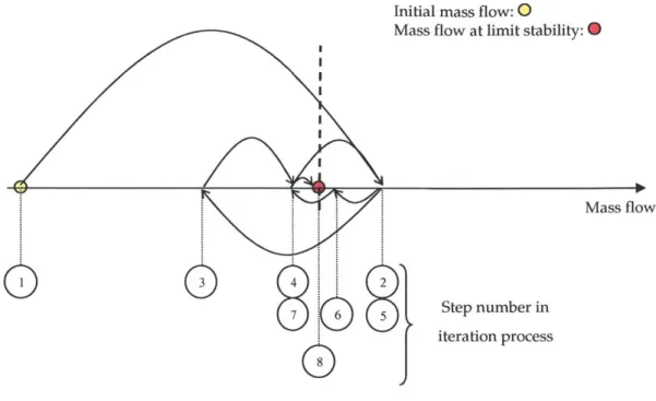
Using the eigenvalue properties above, a method to sweep the compressor characteristic is needed until the point of limit stability is found. Such a method was developed and is illustrated in Figure 2-4, sketching the iterative process as a function of the compressor mass flow. A detailed description of this process is given below.

String of eigenvalues, harmonics 1, 2, 3 and 4 4.3 -. + 2,2-+ 3.2+ 4.2-+ 1.2 + 22+ 5 4.A --523- -45+23 ,7 225 - Slightly unstable 2.5-++ operating point 4.4 +~ 521-3.4 -4 +4 .4- 2.4-05' 03 032 034 0 0Fw 0 4 042 044 046 Fl- 035 wm

Initial mass flow: 0

Mass flow at limit stability: 0

Mass flow

Step number in iteration process

Figure 2-4: Schematic of the search routine to determine the point of limit stability.

The principle is the following: an initial mass flow is given, at which the compression system dynamics are determined, and the eigenvalue belonging to the least stable mode, usually the first harmonic, is found. Depending on the sign of the real part of the eigenvalue (a), that is depending on the system stability, the mass flow is increased or decreased to get closer to the point of limit stability. As soon as a changes sign, meaning that the compression system switched from an unstable configuration to a stable configuration (or vice versa), the step in mass flow is reduced, and the iteration process carries on until the point of limit stability is found.

In the calculation procedure, the following parameters need to be defined:

" initial mass flow * step in mass flow

* tolerance (convergence criterion)

These parameters can be adjusted, depending on the type of compressor, in order to improve the speed of convergence.

2.4

End-Wall Correlations

To refine the mean line calculation and also to be potentially able to use a 3D calculation including end-wall effects as a check, a module computing end-wall losses is implemented. A version of the flow solver MISES extended by Lavainne [9], who implemented end-wall correlations in the calculation, is available. Hence, if one wants to compare the performance of the optimized compressor computed by the optimization loop to the one computed with MISES, end-wall effects on losses need to be implemented inside the optimization loop.

The correlations used are the ones presented by Smith, based on an experimental study of casing boundary layers in multistage axial-flow compressors [13]. The main ideas of these correlations are presented next.

The correlations are based on the hypothesis that the axial velocity distribution along a blade span inside a repeating-stage compressor can be divided into three regions: a free-stream region (modeled by the mean line calculation) and two end-wall-boundary-layer regions. Smith further shows that the end-wall boundary layer thicknesses depend primarily on three quantities: the blade-to-blade passage width, the aerodynamic loading level, and clearances. Correlations are set up to compute this information in order to be able to predict how the pressure-flow and efficiency-flow characteristics are modified by end-wall effects.

To determine the performance of a compressor-stage with end-wall effects, a three-step calculation method is performed:

* First, performance is computed for each stage using the mean line calculation (presented in

section 2.2), ignoring end-wall effects (quantities obtained from this first calculation step are denoted

by tilde (-)).

* Then the end-wall axial velocity boundary layer displacement thicknesses (6*) and end-wall

tangential-force boundary layer thicknesses (v) at hub and tip are computed (the precise definition of these quantities can be found in [13]). The correlations presented by Smith [131 are used to obtain these quantities. They mainly depend on the blade staggered spacing (as defined in Figure 2-5), static pressure rise of the stages, maximum static pressure rise and tip clearance.

e Finally, the efficiency and flow coefficient are computed using the previously calculated

.. compressor blades

Figure 2-5: Definition of the blades staggered spacing (g).

For high hub/tip ratio stages, the efficiency with end-wall effects can be approximated by

1 2

1- ,h . . (2-4)

1_h +Vt h

Similarly, from the flow coefficient computed for the compressor without end-wall effects, the actual flow coefficient can be correlated using the following approximate formula

p I_ I L t I (2-5)

gt g,)h

From the efficiencies and flow coefficients including end-wall effects, it is possible to get the pressure rise across each of the stages. The efficiency and pressure rise obtained from the calculation without end-wall effects are used to compute the isentropic pressure rise (using, the definition of efficiency:q = Vt/Vf isentropic ). Then, using the isentropic pressure rise and the efficiency calculated with

equation (2-4), the definition of the efficiency is used a second time to get the pressure rise with end-wall effects. A flow coefficient shift is finally applied using equation (2-5), yielding the new pressure rise / flow coefficient characteristic. The procedure adopted is sketched next, followed by the explanation of the blade-row loss definition.

Calculation of flow coefficient taking

into account the end-wall effects Calculation of end-wall quantities: S* and v Computation of characteristic including end-wall effects Calculation of ' efficiency taking into account

end-wall effects

Figure 2-6: Calculation procedure implementing end-wall effects.

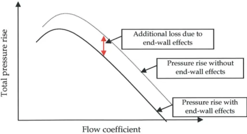
After performing this analysis, one wants to redefine the loss buckets adding the end-wall effects to the originally defined losses. To do so, the definition of the loss coefficient L as used in the dynamic compressor model is:

P - P, ou

L=

P.

pU2

It is possible to compute individual stage loss with end-wall effects using the overall additional blade-row loss due to end-wall effects obtained from the compressor characteristic as shown in Figure

2-7.

--.. Additional loss due to

end-wall effects

Pressure rise with end-wall effects

0

H%

Flow coefficient

Figure 2-7: Additional stagnation pressure loss due to end-wall effects.

(2-6)

Mean flow calculation

The computation of the stage stagnation pressure loss from the overall stagnation pressure loss is obtained by splitting the losses in as many stages as the compressor has. This assumes that the compressor has repeating stages, meaning that the flow pattern is similar in all the stages, hence that the overall additional loss due to end-wall effects can be divided into as many equal parts as there are stages. Then, to compute the blade-row losses from the stages loss, the stage reactions are used

Lrotor L stage * R , (2-7)

Lstator Lstage -(1 - R). (2-8)

Limitations

It has to be kept in mind that the data used to determine the losses due to end-wall effects is limited. Smith [13] reports considerable scatter in the tangential force thickness of hub and casing boundary layers obtained from experimental data. As a consequence, numerical values can be taken within a certain uncertainty range, leading to uncertainties of the performance and stability calculations estimated to 4%.

Furthermore, the data given for the determination of the peak pressure rise coefficient is limited to:

* a Reynolds number of 200,000 * aspect ratios ranging from 2 to 5

* axial gap spacing non-dimensionalized by blade spacing (or pitch), ranging from 0.2 to 0.6 * multistage compressors made up of repeating stages

This means that the results obtained from these correlations are not applicable to compressors with any geometry. Other correlations will have to be applied to include Reynolds number effects and axial gap spacing effects. Concerning the aspect ratio, Smith [141 reports that the applicability of the method to low aspect ratio compressors is of particular concern, and that additional experimental data would be needed to justify the use of the same correlations for these types of low aspect ratio compressors.

Implementation

This section presents results obtained by the mean line calculation with and without end-wall effects. These two different sets of results are compared in Table 2-1 in order to check the relevance of the end-wall effects implementation. Calculations were performed on the 3-stage, repeating stage

compressor (the geometry of this compressor is presented in Appendix B, this particular compressor is used throughout the thesis and is optimized for enhanced stability in Chapter 6).

Overall Pressure Overall adiabatic

Ratio efficiency

Calculation without 1.349 0.936

end-wall effects

Calculation including _1.317

end-wall effects ₀

Table 2-1: Comparison of the 3-stage repeating-stage compressor performance with and without end-wall effects.

Both efficiency and overall pressure ratio follow the expected trend, with a decrease of 2.4% and

1.3% respectively due to losses stemming from end-wall effects.

Note that the level of adiabatic efficiency is high. This is because the secondary loss, that accounts for about 4% of the total loss in a compressor (as will be shown in Figure 3-1), is not taken into account in the calculations. That additional source of loss would yield more realistic values of the adiabatic efficiency, close to 0.88.

Finally, Figure 2-8 presents the losses before and after the end-wall effects are added. These two loss buckets are displayed here to show that the results obtained are reasonable. Although data available comparing blade-row loss buckets with and without end-wall effects are limited, a comparison was done with numerical calculations implementing end-wall effects for similar configurations (for more details, refer to Lavainne [9]). The loss variation due to end-wall effects is of the same order of magnitude in the numerical calculations and in the computations performed with the framework implemented in this thesis.

014

00 - without end-00 _ wall effects

Incidence [0]

Figure 2-8: Loss bucket for rotor 1 of the 3-stage, repeating-stage compressor with and without end-wall correlations.

2.5

Conclusion

This chapter presented the optimization loop. All modules necessary to conduct the performance and stability calculations are defined, together with their limitations and the assumptions made. It was seen how overall pressure ratio, overall adiabatic efficiency and stall margin can be computed

from the input of the geometry and blade-row loss of a compressor, enabling the implementation of the optimization loop.

This tool is used in the next chapters where influence of loss on performance and stability are dissected. The eventual step will be the implementation of this tool for the optimization of the 3-repeating-stage compressor.

Chapter 3

Influence of Blade-Row Losses on

Compressor Performance and Stability

The following two chapters aim at showing the process that was adopted to find a geometric modification of the blade-rows (linked to loss modifications) to be implemented in the optimization framework. This process starts with the exploration and description of the way the shape of a blade-row loss bucket influences compressor performance and stability. The first aim of this chapter is to review mechanisms leading to stagnation pressure loss in turbo-machinery. The second goal is to analytically relate compressor stability to blade-row performance using the Moore-Greitzer model

[11]. The final aim is to demonstrate how each blade-row contributes to the compressor pre-stall

dynamics using the existing dynamic compressor model [15].

3.1

Compressor Characteristics From First Principles

First, some basic definitions are reviewed in order to provide physical insight about blade-row losses and their impact on stability and performance of a given compressor.

Definition of Losses

The end result of losses in turbo-machinery is a rise in entropy and a reduction in stagnation pressure compared to the inlet value or to an ideal value.

The following definitions of the stagnation pressure loss are used:

* total pressure loss coefficient, non-dimensionalized by the blade-row inlet dynamic pressure:

for compressible flow: A

for incompressible flow: w = P Pt2 .t

1

₂

e total pressure loss coefficient used in incompressible dynamic compressor model:

L- Apt _PtlPt2

pU2

pU2

Note that for incompressible flow, stagnation pressure loss is proportional to 1/2 pV 2 and is function of incidence (where incidence is a function of axial and circumferential velocities Vx and V0).

If an IGV fixes the inlet flow angle into a compressor, small changes in Vx and Vo are not independent.

Thus, the flow coefficient (# = Vx /U ) effectively determines the incidence and hence the performance

of a given compressor stage. For this reason, in incompressible flow, the loss as a function of incidence 4i) is equivalent to the loss as a function of flow coefficient L(#).

Several mechanisms lead to stagnation pressure loss in turbo-machinery. One possible breakdown of the overall loss is: profile loss, secondary loss and end-wall loss or annulus loss.

Profile loss is usually taken to be the loss generated in the blade boundary layers well away from the end-walls. The extra loss arising at a trailing edge due to the mixing process of the velocity non-uniformities is usually included as profile loss. Secondary loss arises from the secondary flows that develop in a compressor duct, lead to mixing processes and generate entropy. End-wall loss or annulus loss arises from the end-wall-boundary-layer regions of the blades.

Cumpsty ([31) quotes the estimate for the different loss sources given by Howell (1945), shown here in Figure 3-1.

100- 22% Annulus loss only

4.2% Annulus + secondary loss 80-Annulus + 70 secondary loss + profile loss Flow coefficient

Compressor Characteristic

For the sake of transparency, the example of an incompressible one-stage compressor is taken. From Euler turbine equation, the isentropic total pressure rise across the stage can be written as:

/s = - $(tan#2 + tan a)

The angles in that formula are fixed primarily by the metal angles of the compressor, although they are not strictly constant since the flow undergoes some deviation at the blade-rows exit.

The single-stage compressor pressure rise is obtained from the isentropic pressure rise, subtracting stagnation pressure loss across the rotor (LR) and across the stator (Ls)

y = yVs -LR- LS - .s - L

-The following sketch depicts the influence of losses on the isentropic pressure rise leading to the single-stage compressor characteristic:

"s-s... Loss La+ Ls

os- _{characteristic}

Figure 3-2: Sketch of a compressor characteristic.

Compressor Stability

Compressor stability is directly linked to the loss slopes aL/a. The relation between loss and stability of a compression system was analytically formulated by Moore and Greitzer [111. They modeled a compressor using the following assumptions: all blade-rows are lumped into a single semi-actuator disk, inlet and outlet ducts are infinitely long, and the effects of unsteady loss are neglected. The Moore-Greitzer model has the advantage of being analytically solvable, and the linearized solution to the eigenvalue problem yields for the n" harmonic compressor mode

1V/ts

=- 2 and o An2

n n

X is the blade passage fluid inertia of the rotors, and p of the rotors and stators.

In this simplified case, the compression system is stable (negative growth rate s) for operating points with a negative slope of total-to-static pressure rise coefficient with respect to flow coefficient and unstable for a positive slope (positive growth rate). Although it is not always possible to analytically express the relation between compressor performance and stability like in Moore-Greitzer model, the modes of a compression system and the blade-row performance are always coupled. This is because the compression system dynamics consist of pre-stall modes affected by the background flow field, driven by the blade-row performance.

Conclusion

Recalling Figure 3-2 and the expression of the growth rate obtained from Moore-Greitzer model, the effects of changes in loss on compressor performance and stability are as follows: a shift of the loss level will have an impact on performance (y will be changed) but stability, directly linked to the slopes ( BL/8$ ), will not be affected. On the other hand, a modification of blade-row operating range (incidence range between two points where losses are twice the minimum losses -this expression is used to describe the width of the loss buckets) will change the slopes distribution ( aL/8# ) and eventually affect compressor stability.

3.2

Demonstration of Blade-Row Contribution to Compressor

Dynamics

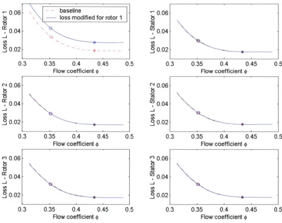
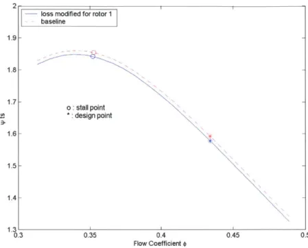
In this section, the dynamic compression system model is implemented as well as the mean line calculation presented in Chapter 2. Results presented were obtained for the 3-stage, repeating-stage compressor where the geometry is given in Appendix B. Changes in the loss distribution of the first-stage-rotor are studied in order to assess the contribution of blade-row performance on the compressor dynamics.

Introduction of a Loss Level Change: Performance is Altered, not Stability

This section presents the results of a loss bucket modification for rotor 1 of the 3-stage compressor in terms of loss level. A bias Aei was artificially introduced on the loss bucket of rotor