A simple extension of FFT-based methods to strain gradient loadings - Application to the homogenization of beams and plates

HAL Id: hal-02942202

https://hal.archives-ouvertes.fr/hal-02942202v2

Preprint submitted on 23 Dec 2020

HAL is a multi-disciplinary open access archive for the deposit and dissemination of sci-entific research documents, whether they are pub-lished or not. The documents may come from teaching and research institutions in France or abroad, or from public or private research centers.

L’archive ouverte pluridisciplinaire HAL, est destinée au dépôt et à la diffusion de documents scientifiques de niveau recherche, publiés ou non, émanant des établissements d’enseignement et de recherche français ou étrangers, des laboratoires publics ou privés.

A simple extension of FFT-based methods to strain

gradient loadings - Application to the homogenization of

beams and plates

Lionel Gélébart

To cite this version:

Lionel Gélébart. A simple extension of FFT-based methods to strain gradient loadings - Application to the homogenization of beams and plates. 2020. �hal-02942202v2�

A simple extension of FFT-based methods to strain gradient loadings –

Application to the homogenization of beams and plates

Lionel Gélébart

CEA Paris-Saclay, DEN/DMN/SRMA, 91191, GIF/YVETTE, FRANCE Email : lionel.gelebart@cea.fr

Abstract:

Because of their simplicity, efficiency and ability for parallelism, FFT-based methods are very attractive in the context of numerical periodic homogenization, especially when compared to standard FE codes used in the same context. They allow applying to a unit-cell a uniform average strain with a periodic strain fluctuation that is an unknown quantity. Solving the problem allows to evaluate the complete stress-strain fields.

The present work proposes to extends straightforwardly the method from uniform loadings (i.e. uniform applied strain) to strain gradient loadings (i.e. strain fields with a uniform strain gradient) and proposes an application to the homogenization of beams and plates, while keeping the simplicity of the original method. It is observed that, due to the use of periodic boundary conditions, among the 18 strain gradient components, only 9 can be really prescribed. The identification of a subset of strain gradient loadings allows for a minimally invasive modification of the iterative algorithm so that the implementation is straightforward. In spite of a reduced subset of 9 independent loadings among the 18 available, the second part of the paper demonstrates that it is enough for considering the homogenization of beams and plates. A first application validates the approach and compares it to another FFT-based method dedicated to the homogenization of plates. The second application concerns the homogenization of beams, for the first time considered (to author’s knowledge) with an FFT-based solver. The method applies to different beam cross-sections and the proposition of using composite voxels drastically improves the numerical solution when the beam cross-section is not conform with the spatial discretization, especially for torsion loading.

As a result, the massively parallel AMITEX_FFTP code has been slightly modified and now offers a new functionality, allowing the users to prescribe torsions and flexions to beam or plate heterogeneous unit-cells.

Keywords :

1 – Introduction

The present paper lies in the overall framework of numerical homogenization of heterogeneous materials for which the mechanical behavior at the upper scale derives from spatial averages of stress-strain fields simulated on heterogeneous unit-cells. The first developments and most common applications focus on first order homogenization, the homogenized behavior relating the displacement gradient tensor to a stress tensor, or more specifically, under the small perturbations assumption, the linearized strain to the Cauchy stress. The type of boundary conditions applied to the unit-cell is quite important in that context. First, they must satisfy the Hill-Mandel condition so that the average microscopic strain energy is equal to the macroscopic one. Then, various choices satisfying this condition are available: Kinematic Uniform Boundary Conditions, Stress Uniform BC, periodic BC or even normal-mixed BC [15]. If the choice of periodic BC is obvious for periodic microstructures, it also provides the best estimate for random microstructures [23] [9] compared to KUBC or SUBC, that provide upper and lower bounds (at least for linear material) [19]. If applying PBC is not straightforward in Finite Element codes and can deteriorate the computation performance, it is natural for the FFT-based methods proposed in the 1990’s [27].

These methods have been extensively used and improved during the last decade, reducing the initial drawbacks such as convergence issues for highly contrasted materials, spurious oscillations or sensitivity of the convergence to the reference material behavior (an algorithm parameter). Among significant improvements: modified discrete Green operators reducing spurious oscillations and improving the convergence ([4], [31] [29],…), algorithms replacing the initial fix-point algorithm to improve convergence ([32], [16], [20], [11] …) or composite voxels accounting for multi-phase materials, for voxels crossed by an interface, to improve the numerical solution and reduce spurious oscillations ([4], [17], [22] …). The list is not exhaustive and numerous theoretical works reinforce the mathematical basis of the method.

Due to their high numerical efficiency compared to finite element codes used in the same context (periodic boundary conditions), various works intend to extend the method to various applications. Among these applications, we can cite the extension to non-local behaviors such as strain gradient plasticity [26] or damage phase field [11], the coupling with metallurgical phase fields such as martensitic phase transformation [24] or other physics such as magneto-electricity [3], the coupling with DD codes [2]… Once again, this short list is far from exhaustive but gives an idea of the increasing development of the method towards new research fields.

Another kind of extension concerns higher order numerical homogenization [30][12]. In that case, the homogenized behavior is not only dependent of the first gradient of the displacement but also of higher order terms. Following this idea of going beyond the classical application of an average strain loading (i.e. first order displacement gradient) the present paper lies in the same general context. Actually, it focuses on the extension to average strain gradient loadings (i.e. second order displacement gradient), with an additional constraint of simplicity for the implementation. In other words, in the first part of the paper, the question is to propose a method to apply strain gradient loadings within classical FFT-based codes, initially designed for first gradient loadings, with a minimally invasive modification. If the set of strain gradient loadings fulfilling this constraint is

reduced, the second part of the paper demonstrates that it is still large enough to deal with the question of beams and plates numerical homogenization with FFT-based algorithms.

The first part of the paper proposes a straightforward extension of the classical FFT-based method in order to account for strain gradient loadings. It is observed that, due to the use of periodic boundary conditions, among the 18 strain gradient components, only 9 can be applied. The second part of the paper demonstrates its ability to solve the question of the homogenization of beams and plates. Actually, the questions of beams and plates homogenization can be regarded as second order term homogenizations [13] for which strain gradients are associated to flexion and torsion loadings. For plates, if the classical numerical implementation relies on the finite element method [13] [18], Nguyen also proposes an FFT-based method devoted to this application [28]. It relies on a specific algorithm combined with a dedicated Green operator to account for the traction free boundary conditions applied at the plates’ free surfaces. On the contrary, if the finite element method has also been used is also used for beams homogenization [7], to the best of author’s knowledge, FFT-based methods have never been proposed in that context. One purpose of the paper is then to demonstrate that the same slightly modified FFT-based code can be used for both classical (i.e. first gradient term), as well as beams and plates, numerical periodic homogenization. This is made possible and quite efficient since recent FFT-based methods (see beginning of the introduction) allow for the simulation of unit-cells enlarged with void voxels (i.e. infinite contrast) to account for traction free boundary conditions.

To sum up, the first part of the paper (section 2) introduces the simple extension of the FFT-based method to a reduced set of strain gradient loadings and the second part (section 3) applies the method to the homogenization of beams and plates. In this part, the first sub-section presents the application to plates homogenization and focuses on the comparison with Nguyen’s method using exactly the same cases [28]. Finally, the second sub-section presents the new FFT-based application to beams homogenization with an additional emphasis on the use of composite voxels when the beam cross-section is not conform with the regular grid discretization.

2 – Simple extension of the FFT-based method to strain gradient loadings

Sub-section 2.2 introduces the standard FFT-based algorithm after a small discussion on the different descriptions of the periodicity condition in sub-section 2.1, useful in sub-section 2.3 introducing the simple extension to strain gradient loadings. A final sub-section extends the idea from the small perturbation to the finite strains framework.

2.1 : Periodicity condition

The description of the periodicity condition prescribed on a unit-cell Ω can be done equivalently from two different points of view.: whether the unit-cell Ω is considered alone or an infinite periodic medium Ω is considered. In the first case, fields are defined on Ω and boundary conditions have to be applied on its boundary ∂Ω. In the second case, fields are defined on an infinite space and

Ω −periodicities are assumed for the fields. The first description is more appropriate for Finite-Element solvers, the second is well-suited for FFT-based solvers. The two equivalent descriptions of the equilibrium condition, submitted to a periodicity condition, are given in equation (1). Below,

“𝜎. 𝒏 antiperiodic on ∂Ω” means that the traction vector (𝜎. 𝒏) on opposite points of opposite faces of Ω are opposite. 𝒅𝒊𝒗(𝜎(𝒙)) = 0 𝜎. 𝒏 antiperiodic on ∂Ω ⟺ 𝒅𝒊𝒗(𝜎(𝒙)) = 0 𝜎 Ω − periodic (1)

The periodicity condition of a displacement field 𝒖 in equation (2) is also equivalently formulated on Ω in terms of strain field 𝜀̃, adding a compatibility in that case. Below, “𝒖 periodic on ∂Ω” means that the displacement 𝒖 evaluated on opposite points of opposite faces are equal.

𝒖 periodic on ∂Ω ⟺ 𝒖 Ω − periodic ⟺ 𝜀̃ compatible _{𝜀̃ Ω − periodic} (2)

2.2 : FFT-based algorithm

When considering classical (i.e. first order term) periodic homogenization under the small perturbations assumption, the problem to solve (3) consists of a heterogeneous unit cell Ω described by its stiffness tensor field 𝑐, submitted to an average displacement (first order) gradient ∇𝑼 with periodic boundary conditions. The displacement field is written as the sum of the prescribed linear term and the unknown fluctuation field 𝒖.

⎩ ⎪ ⎪ ⎨ ⎪ ⎪ ⎧𝒅𝒊𝒗(𝜎(𝒙)) = 0 𝜎(𝒙) = 𝑐(𝒙): 𝜀(𝒙) 𝜀(𝒙) = (∇𝒖) (𝒙) 𝒖(𝒙) = ∇𝑼. 𝒙 + 𝒖(𝒙) 𝒖 periodic on ∂Ω 𝜎. 𝒏 antiperiodic on ∂Ω (3)

Using equations (1) and (2), this problem (3) written on Ω, is equivalent to problem (4) written on Ω , removing the 𝒙 dependence for the sake of concision, the average strain 𝐸 being equal to the symmetrized average gradient (𝐸 = (∇𝑈) ).

⎩ ⎪ ⎨ ⎪ ⎧𝒅𝒊𝒗(𝜎) = 0_{𝜎 = 𝑐: 𝜀} 𝜀 = 𝐸 + 𝜀̃ 𝜀̃ compatible 𝜀̃ Ω − periodic 𝜎 Ω − periodic (4)

Now, introducing a homogeneous reference stiffness 𝑐 allows to define equivalently the problem (5). ⎩ ⎪ ⎨ ⎪ ⎧𝒅𝒊𝒗(𝑐 : 𝜀 + 𝜏) = 0_{𝜏 = 𝑐: 𝜀 − 𝑐 : 𝜀̃} 𝜀 = 𝐸 + 𝜀̃ 𝜀̃ compatible 𝜀̃ Ω − periodic 𝜎 = 𝑐 : 𝜀̃ + 𝜏 Ω − periodic (5)

Temporarily assuming the so-called polarization 𝜏 as a known Ω −periodic field, allows defining the auxiliary problem (6) which can be solved by the application of the Green operator Γ ,

straightforward in Fourier space as the stiffness 𝑐 is homogeneous (see the annex of [27] for a detailed description). 𝜀̃ = −Γ ∗ 𝜏 (⇄ Fourier) ⇔ 𝒅𝒊𝒗(𝑐 : 𝜀̃ + 𝜏) = 0 𝜀̃ compatible 𝜀̃ Ω − periodic 𝜎 = 𝑐 : 𝜀̃ + 𝜏 Ω − periodic (6)

Finally, the initial problem (4), equivalent to problem (5), reduces to problems (6) and (7). Note that periodicity and compatibility conditions are gathered in problem (6) and automatically fulfilled when applying the Green operator in Fourier space, so that problem (7) gathers a set of equations, which, followed step by step, defines the simple fix-point algorithm proposed initially by Moulinec and Suquet [27]. Initializing the strain field 𝜀 (with 𝜀 = 𝐸) allows to evaluate the polarization field 𝜏 (7)a.

Then, the Green operator applies (in Fourier space) on the polarization to evaluate the fluctuation strain field 𝜀̃ (7)b, which, added to the average (applied) strain field provides the strain field 𝜀 (7)c (in

practice it can be done easily in Fourier space on the null frequency). This strain field allows to begin a second iterate and so on until convergence.

𝜏 = 𝑐: 𝜀 − 𝑐 : 𝜀̃ (𝑎) 𝜀̃ = −Γ ∗ 𝜏 (⇄ Fourier) (𝑏) 𝜀 = 𝐸 + 𝜀̃ (𝑐)

(7)

2.3 : A straightforward extension to strain gradient loadings with a simple implementation

The purpose of this section is to add a compatible non-uniform applied strain 𝜀∗ _{to the homogeneous}

applied strain 𝐸, modifying the initial problem (4) in problem (8).

⎩ ⎪ ⎨ ⎪ ⎧𝒅𝒊𝒗(𝜎) = 0_{𝜎 = 𝑐: 𝜀} 𝜀 = 𝐸 + 𝜀∗_{+ 𝜀̃} 𝜀̃ compatible 𝜀̃ Ω − periodic 𝜎 Ω − periodic (8)

Following the different steps introduced in section 2.2, problem (8) is equivalent to problem (9) below. It depicts a fix-point algorithm (succession of steps (a)->(b)->(c)->(a)->(b)…). The single and simple difference with algorithm (7) is step (c) with the addition of the applied strain field 𝜀∗_.

In addition, for the sake of simplicity, we would like to use exactly the same algorithm as described by problems (6) and (7) with a minor modification that consists in adding the non-uniform applied strain 𝜀∗ _{when evaluating the strain in equation (7)}

𝜏 = 𝑐: 𝜀 − 𝑐 : 𝜀̃ (𝑎) 𝜀̃ = −Γ ∗ 𝜏 (⇄ Fourier) (𝑏) 𝜀 = 𝐸 + 𝜀∗+ 𝜀̃ (𝑐)

(9)

Among the compatible non-uniform applied strain fields 𝜀∗_{, the simplest ones are linear fields.}

Actually, the compatibility condition, that involves double derivations of the strain components, is satisfied as the double derivations automatically vanish for linear fields. In the following, the heterogeneous applied strain fields are limited to such linear fields characterized by their strain gradients 𝐺 as follows, assuming (𝒙 =0) the center of the unit-cell:

𝜀∗(𝒙) = 𝐺. 𝒙 or 𝜀∗ _{= 𝐺 𝑥 (10)}

Note that 𝐺 is symmetric w.r.t. its first two indices (due to the symmetry of the strain tensor) so that it consists of 6x3=18 components.

The question is now to identify a set of applied strain fields 𝜀∗ _{for which problem (8) reduces to}

problems (6) and .

The first constraint arises from the compatibility equation (8)4 of the strain field (8)3 in problem (8).

Hence, the applied heterogeneous strain 𝜀∗ _{must be compatible. Among the compatible fields, the}

simplest ones are linear fields. Actually, the compatibility condition, that involves double derivations of strain components, is satisfied as the double derivations automatically vanish for linear fields. In the following, the heterogeneous applied strain fields are limited to such linear fields characterized by their strain gradients 𝐺 as follows, assuming (𝒙 =0) the center of the unit-cell:

𝜀∗_{(𝒙) = 𝐺. 𝒙 or 𝜀}∗ _{= 𝐺 𝑥}

The second constraint comes from the application of the Green operator in problem b. Actually,

applying the Green operator is equivalent to solve the auxiliary problem (6), derived from problem (4). Instead, the auxiliary problem derived from problem (8) should have read:

𝒅𝒊𝒗(𝑐 : 𝜀̃ + 𝑐 : 𝐺. 𝒙 + 𝜏) = 0

𝜀̃ compatible 𝜀̃ Ω − periodic 𝜎 = 𝑐 : 𝜀̃ + 𝑐 : 𝐺. 𝒙 + 𝜏 Ω − periodic

Hence, the only way to use the auxiliary problem (6) instead of the auxiliary problem is to have the term 𝑐 : 𝐺. 𝒙 equilibrated (𝒅𝒊𝒗(𝑐 : 𝐺. 𝒙) = 0) and the term (𝑐 : 𝜀̃ + 𝑐 : 𝐺. 𝒙 + 𝜏) Ω −periodic. 𝜀̃ and 𝜏 being Ω −periodic, the second condition on 𝐺 corresponds to the Ω −periodicity of 𝑐 : 𝐺. 𝒙. Following equation (1), these two conditions on Ω are now written on Ω as follows:

𝒅𝒊𝒗(𝑐 : 𝐺. 𝒙) = 0

𝑐 : 𝐺. 𝒙 Ω − periodic ⟺

𝒅𝒊𝒗(𝑐 : 𝐺. 𝒙) = 0

Assuming an isotropic behavior for 𝑐 , with Lamé coefficients 𝜆 and 𝜇 , the first condition on 𝐺 (𝒅𝒊𝒗(𝑐 : 𝐺. 𝒙) = 0), expressed in Cartesian coordinates, reads:

𝜆 (𝐺 + 𝐺 + 𝐺 ) + 2𝜇 (𝐺 + 𝐺 + 𝐺 ) = 0 𝜆 (𝐺 + 𝐺 + 𝐺 ) + 2𝜇 (𝐺 + 𝐺 + 𝐺 ) = 0 𝜆 (𝐺 + 𝐺 + 𝐺 ) + 2𝜇 (𝐺 + 𝐺 + 𝐺 ) = 0

The second condition is the anti-periodicity of (𝑐 : 𝐺. 𝒙). 𝒏 on opposite faces of Ω, it reads: 𝜆 (𝐺 + 𝐺 + 𝐺 ) + 2𝜇 𝐺 = 0 𝐺 = 0 𝐺 = 0 𝐺 = 0 𝜆 (𝐺 + 𝐺 + 𝐺 ) + 2𝜇 𝐺 = 0 𝐺 = 0 𝐺 = 0 𝐺 = 0 𝜆 (𝐺 + 𝐺 + 𝐺 ) + 2𝜇 𝐺 = 0

It is clear that the set equations is automatically satisfied as soon as is fulfilled. Hence, gathers the 9 constraints that must be satisfied by 𝐺 if we want to solve problem (8), with an applied strain

gradient 𝜀∗_{(𝒙) = 𝐺. 𝒙, using the very simple algorithm described by problem . In other words, among}

the 18 coefficients of 𝐺, 6 coefficients 𝐺 (with i ≠ j ) must be set to zero, nine coefficients 𝐺 are constrained by 3 equations and the coefficients 𝐺 (with i ≠ j, a ≠ k and k ≠ i) are free. The coefficients 𝐺 (with i ≠ j ) can be associated to bending loadings and the coefficients 𝐺 (with i ≠ j, a ≠ k and k ≠ i) to torsion loadings.

2.4 : Restrictions on the applied strain gradient

It must be emphasized that among the 18 components of the applied strain gradient only 9 can really be applied in this context of periodic boundary conditions. Mathematical foundations can be found in Annex A. For any 𝐺 applied strain gradient, a periodic and compatible fluctuation displacement component 𝑢 can be found that modifies its effect. For example, a fluctuation displacement 𝑢 = 𝐺 𝑥 can modify the effect of the applied strain gradient 𝐺 . Actually, 𝑢 satisfies the periodicity condition (i.e 𝑢 = 𝑢 − , with ℎ the cell size in direction 2) and it is associated to a fluctuation strain field 𝜀̃ = 𝐺 𝑥 , so that the average strain gradient seen by the unit-cell is not 𝐺 but 𝐺 + 𝐺 . Hence, these strain gradient components ijj cannot be prescribed, they are results of the simulation.

Note that this property has been validated in our FFT-based implementation (algorithm (9)) on a simple homogeneous unit-cell: the resulting stress and strain fields remain homogeneous and independent of the applied strain gradient components 𝐺 .

The nine remaining components are associated to six bending loadings (components 𝐺 with 𝑖 ≠ 𝑗) and three torsion loading (components 𝐺 with 𝑖 ≠ 𝑗, 𝑖 ≠ 𝑘, and 𝑗 ≠ 𝑘).

2.5 : Implementation considerations

Considering an existing FFT-based code able to solve problem (7), transforming this code to solve problem (9) is obvious. It consists in adding the applied strain gradient field when adding the

homogeneous applied strain field to the periodic strain fluctuation. This is done, first when initializing the strain field (with a null fluctuation) and then, at the end of each iteration. The impact on the memory footprint is null, as no additional field needs to be allocated, and the additional computational cost is low compared to the complete cost of an iteration.

The implementation of the algorithm is provided below. Note that during the loops, 𝜀̃ stores the strain fluctuation added to the average strain 𝐸 (using 𝜀̃ (0) = 𝐸). In addition to this fix point algorithm, a convergence acceleration procedure is implemented in the code AMITEX_FFTP [1]. Its description can be found in [10]. It consists of storing 𝑁 couples of solutions (𝜀 ) and residual (𝜀 − 𝜀 ) associated to the last four iterations, and, every 𝑛 iterations, propose a solution deduced from a combination of the stored solutions (in AMITEX_FFTP, 𝑁=4 and the default value for 𝑛 is 3).

𝑖𝑛𝑖𝑡𝑖𝑎𝑙𝑖𝑧𝑒 ∶ 𝜀 = 𝐸 + 𝜀∗ 𝜀̃ = 0 𝑙𝑜𝑜𝑝: 𝜎 = 𝑐: 𝜀 𝜎 = 𝐹𝐹𝑇(𝜎) 𝜀̃ = −Γ : 𝜎 − 𝑐 : 𝜀̃ 𝜀̃ (0) = 𝐸 𝜀̃ = 𝑖𝐹𝐹𝑇 𝜀̃ 𝜀 = 𝜀̃ + 𝜀 ∗ (11)

2.6 : Extension to finite strain

Even if not applied in the present paper, an extension to the general framework of finite strains is proposed below.

The extension of the FFT-based method to finite strain proposed initially by Lahellec [25] is quite straightforward, replacing in problems (5) and (6), the Cauchy stress 𝜎 by the first Piola-Kirchoff stress 𝜋, and strain field 𝜀 by the displacement gradient ∇𝑢, the divergence and gradient operators now acting on the initial configuration. The main difference is that these tensors are no more symmetric and involve nine components. Then, the reasoning proposed to account for heterogeneous loadings, under the small perturbation assumption in the previous section, is straightforwardly extendable at finite strain. For the sake of conciseness, we focus on the main ingredients but not recall the complete reasoning below.

The problem to solve at finite strain, accounting for a heterogeneous applied displacement gradient ∇𝑢∗_{, reads:}

⎩ ⎪ ⎪ ⎨ ⎪ ⎪ ⎧𝒅𝒊𝒗(𝜋) = 0_{𝜋 = 𝑐(∇𝑢)} ∇𝑢 = ∇𝑈 + ∇𝑢∗+ ∇𝑢 ∇𝑢 compatible ∇𝑢 Ω − periodic 𝜋 Ω − periodic (12)

A simple way to satisfy the compatibility condition for ∇𝑢∗ _{is to choose a strain gradient field (13)}

characterized by the tensor 𝐺, which is no more symmetric on its two first indices when considering the finite strain context.

∇𝑢∗_{(𝒙) = 𝐺. 𝒙 or ∇𝑢}∗ _{= 𝐺 𝑥 (13)}

Then, the simple fixed-point algorithm described by problem (14) to solve problem (12) at finite strain is very close to the algorithm (9) used to solve the problem with the small perturbations approximation. Note that here, the Green operator is different from the one introduced in equation (6) as it now applies to non symmetric tensors.

Then, solving problem (12) with the simple fixed-point algorithm described by problem (14) is possible if the applied strain gradient satisfies the same constraints as , with a non-symmetric 𝐺.

𝜏 = 𝑐(∇𝑢) − 𝑐 : ∇𝑢

∇𝑢 = −Γ ∗ 𝜏 (⇄ Fourier) ∇𝑢 = ∇𝑈 + ∇𝑢∗_{+ ∇𝑢}

(14)

As the set of equations does not account for the symmetry of 𝐺, it applies equivalently to the non-symmetric 𝐺. Now, the space of available loading has 18 dimensions (27 components minus 9 equations) instead of 9 under the small strain assumption (18 components minus 9 equations).

2.6 : Conclusion

This work of FFT-based codes, classically implemented to account for uniform applied strain, to account for linearly varying applied strains (i.e. with a constant applied strain gradient). The modification is extremely simple and has a null memory footprint.

The price to pay for this simplicity is a constraint on the components of the applied strain gradient: among the 18 components (or 27 at finite strain) of the strain gradient, 9 equations reduce the space of available loadings to 9 dimensions (or 18 at finite strain). However, the next section will demonstrate that it is enough to consider the problems of the homogenization of beams and plates.

3 : Application to the homogenization of beams and plates

The purpose of this section is to demonstrate that the slight modification proposed in the previous section, applied to an existing FFT-based code that is able to simulate microstructures with null

elastic properties, is enough to consider the problem of thin plates or elongated beams

homogenization. Nguyen [28] has initially addressed the question of thin plates homogenization with an FFT-based solver, but his approach relied on a dedicated Green operator whereas our approach relies on the standard Green operator. and any FFT-based solver able to account for null elastic properties. For the sake of validation and comparison, section 3.1 reproduces all the simulation cases proposed by Nguyen [28]. Then, section 3.2 extends the approach to the

homogenization of beams, treated for the first time, to the author’s knowledge, with an FFT-based solver.

As the convergence properties reported below (section 3.1 and 3.2) depends on the FFT-based code used for the simulation, a brief description is necessary. The two main features influencing the convergence properties in our code AMITEX_FFTP [1] are the iterative algorithm and the discrete Green operator. First, the algorithm corresponds to the fixed-point algorithm [27], described by problem (7), combined with an Anderson convergence acceleration technique reported in ([10], section 3.2.1). This acceleration technique drastically improves the fixed-point algorithm

convergence. In addition, compared to the Newton-Raphson implementation also proposed for FFT-based solvers with non-linear behaviors [14], it is interesting because it does not require the tangent matrix behavior, whose analytical evaluation may be tedious. On the other hand, the memory footprint is higher: our implementation requires four couples of (solution field, residual field). Second, the discrete Green operator is associated to a finite element discretization with linear hexaedral elements with reduced integration [31] [29]. It is efficient to reduce spurious oscillations and improve convergence. Thanks to these two elements, the code is able to account, quite efficiently, for unit-cells containing void voxels (null elastic properties).

3.1 : Homogenization of plates

The purpose of this section is to demonstrate that a general FFT-based code, equipped with the minor modification proposed in this study, extends its application domain to the homogenization of plates. Validation comes from comparisons with analytical results and numerical results obtained by Nguyen [28]. Note that an extensive and refined comparison between our simulations and Nguyen’s simulations is not easy because of the differences between the iterative algorithms, the discrete Green operators and the convergence criterion. Especially, the convergence criterion used by Nguyen is a ‘macroscopic’ criterion based on the ‘relative’ difference of the strain energy between two iterations whereas the criterion used in AMITEX_FFTP relies on the ‘absolute’ equilibrium condition of the ‘local’ stress field.

3.1.1 : Method

3.1.1.1 : General setting

We consider a thin heterogeneous plate described by a unit cell Ω periodically repeated in the plane (𝒆𝟏, 𝒆𝟐), with direction (𝒆𝟑) normal to the plate. Assuming an applied strain field consistent with the

⎩ ⎪ ⎨ ⎪ ⎧𝒅𝒊𝒗(𝜎) = 0_{𝜎 = 𝑐: 𝜀} 𝜀 = 𝐸 + 𝜒𝑥 + (∇𝒖) 𝒖 periodic on ∂ Ω 𝜎. 𝒏 antiperiodic on ∂ Ω 𝜎. 𝒏 = 0 on ∂ Ω (15)

Where ∂ Ω denotes the four faces of normal directions (𝒆𝟏) and (𝒆𝟐), submitted to periodic

boundary conditions and ∂ Ω the two faces submitted to a traction-free boundary condition. The macroscopic applied strain and strain gradient are limited to the in-plane components for both the uniform and non-uniform parts, in bold in equation (16) The prescribed components of both the average strain 𝐸 and strain gradient 𝜒 are limited to the in-plane components (see Annex A.4 for a detailed description of prescribed and ‘measured’ components). However, d Note that, due to mechanical couplings between directions, the out of plane components do not systematically vanish (i.e. even in the simplest case of an elastic, homogeneous and isotropic material, the components 𝐸 and 𝜒 arise from the classical Poisson effect). These out-of-plane components, that are not prescribed, can be evaluated as a post-treatment of the simulation. Note that problem (15) is exactly the same as proposed in ([28] equations 32 and 33) but they mention that the out-of-plane

components 𝑜𝑓 𝐸 and 𝜒 are prescribed to 0. The author’s opinion is that prescribing these quantities is not consistent with the stress free boundary condition applied on the upper and lower plate surfaces (i.e. 𝜎. 𝒏 = 0 on ∂ Ω). For example, the transverse strain 𝐸 (but also 𝜒 ) arising when applying a uniaxial strain 𝐸 depends on the Poisson coefficient and cannot be set to 0. As observed in section 3.2.1, the numerical results obtained with the present approach are consistent with the analytical and numerical results given in [28] for heterogeneous plates.

𝐸 = 𝑬𝟏𝟏 𝑬𝟏𝟐 𝐸 𝑬𝟏𝟐 𝑬𝟐𝟐 𝐸 𝐸 𝐸 𝐸 and 𝜒 = 𝝌𝟏𝟏 𝝌𝟏𝟐 𝜒 𝝌𝟏𝟐 𝝌𝟐𝟐 𝜒 𝜒 𝜒 𝜒 = 𝑮𝟏𝟏𝟑 𝑮𝟏𝟐𝟑 𝐺 𝑮𝟏𝟐𝟑 𝑮𝟐𝟐𝟑 𝐺 𝐺 𝐺 𝐺 (16) 3.1.1.2 : FFT-based resolution on an enlarged unit-cell Ω∗

In their paper, to solve problem (15), Nguyen and al. [28] follow exactly the reasoning described in section 2. However, keeping the traction-free condition on ∂ Ω, they have to modify the Green operator to account for this condition in the auxiliary problem.

Instead, In the present paper, instead of solving problem (15) with a modified Green operator, we solve problem (9) with the classical periodic Green operator, built with full periodic conditions, available in every FFT-based codes. In order to satisfy the traction-free boundary condition that appears in problem (15) but not in problem (9), the fully periodic problem is not solved on the unit-cell Ω but on an enlarged unit-unit-cell Ω∗ _{adding to Ω one layer with null elastic properties on each side}

of ∂ Ω (see Figure 1). In practice the added layers are one voxel thickness in the discretized problem and using one layer on each side allows to keep the same middle surface for Ω and Ω∗ _{(helpful for the}

post-treatment of the stress field). Due to the added void layers, the in-plane components of 𝐸∗ _and

𝜒∗ _{applied to Ω}∗ _{are the same as applied to the sub-domain Ω must be the same but the out of plane}

components of 𝐸∗ _{and 𝜒}∗_{, can be chosen arbitrarily. For the out-of-plane components of 𝜒}∗_{, i.e.}

𝐺∗ , , it has been demonstrated in section 2.4 (and Annex A) that these components cannot be prescribed with periodic boundary conditions. Their value can be arbitrarily set to 0.

𝐸∗₌ 𝑬_𝑬𝟏𝟏 𝑬𝟏𝟐 0 𝟏𝟐 𝑬𝟐𝟐 0 0 0 0 and 𝜒∗₌ 𝝌_𝝌𝟏𝟏 𝝌𝟏𝟐 0 𝟏𝟐 𝝌𝟐𝟐 0 0 0 0 = 𝑮𝟏𝟏𝟑 𝑮𝟏𝟐𝟑 0 𝑮𝟏𝟐𝟑 𝑮𝟐𝟐𝟑 0 0 0 0 (17) To clarify this point, let’s consider the 22 in-plane component and the 33 out-of-plane component successively. Let 𝜀̅∗ _{(𝑥 , 𝑥 ) be the linear average strain (component 22) in direction 2 so that ∀𝒙 ∈}

Ω∗_{, 𝜀̅}∗ _{(𝑥 , 𝑥 ) = 𝐸}∗ _{+ 𝐺}∗ _{𝑥 (the linear average contribution of strain fluctuation 𝜀̃ vanishes).}

As, the linear average in direction 2 is performed in a single domain (whether Ω or in the void) then 𝜀̅ (𝑥 , 𝑥 ), the linear average strain in the domain Ω, follows the same relation 𝜀̅ (𝑥 , 𝑥 ) = 𝜀̅∗ _{(𝑥 , 𝑥 ) = 𝐸 + 𝐺 𝑥 with 𝐸 = 𝐸}∗ _{and 𝐺 = 𝐺}∗ _{. In other words, the macroscopic}

components (𝐸 and 𝐺 ) applied to Ω are the same as the macroscopic components applied to Ω∗

(𝐸∗ _{and 𝐺}∗ _{). Same idea can be followed with components 11 and 12.}

Now, 𝜀̅∗ _{(𝑥 , 𝑥 ) is the linear average strain (component 33) in direction 3 so that ∀𝒙 ∈}

Ω∗, 𝜀̅∗ (𝑥 , 𝑥 ) = 𝐸∗ . In that case, 𝜀̅ (𝑥 , 𝑥 ), the linear average strain in the domain Ω, is different from 𝜀̅∗ _{(𝑥 , 𝑥 ) as 𝜀̅}∗ _{(𝑥 , 𝑥 ) = 𝑓𝜀̅ (𝑥 , 𝑥 ) + (1 − 𝑓)𝜀̅ (𝑥 , 𝑥 ), where 𝜀̅ (𝑥 , 𝑥 )}

represents the linear average strain in the void layers and 𝑓 the volume fraction of Ω in Ω∗_{. As a}

consequence, 𝜀̅ (𝑥 , 𝑥 ) ≠ 𝐸∗ _{and then 𝐸 ≠ 𝐸}∗ _{. In other words, the additional void layers are}

free to deform so that the average 𝐸∗ _{can be chosen arbitrarily. Same idea can be followed with}

components 13 and 23.

Finally, as the out-of-plane components of 𝜒∗ _{cannot be prescribed on Ω}∗ _{(see section 2.4 and Annex}

A), obviously, they cannot be prescribed on Ω (a subset of Ω∗_).

To make short: in-plane components of 𝐸∗ _{and 𝜒}∗_{, prescribed on Ω}∗_{, are also prescribed on Ω. On}

the other hand, the out-of-plane components of 𝐸 and 𝜒 cannot be prescribed on Ω but can be evaluated as post-treatments.

In order to use the method proposed in the previous section to account for linearly varying applied strain, the strain gradient components imposed in equation (17) have to satisfy the constraints established in the general case (set of equations ). In the present case, the imposed component 𝐺 remains unconstrained; it consists of an elementary torsion plate loading. The unique constraint applies to the 𝐺 components:

𝜆 (𝐺 + 𝐺 + 𝐺∗ ) + 2𝜇 𝐺∗ _{= 0}

This constraint allows proposing two elementary flexion plate loadings, governed by the components 𝐺 and 𝐺 applied to Ω, as follows:

⎩ ⎨ ⎧𝐺_𝐺 imposed_{= 0} 𝐺∗ = − 𝜆 𝜆 + 2𝜇 𝐺 ⎩ ⎨ ⎧𝐺_{𝐺 imposed}= 0 𝐺∗ = − 𝜆 𝜆 + 2𝜇 𝐺

It is worth noting that 𝐺∗ _{, the gradient of 𝜀 according to 𝑥 is applied to Ω}∗ _{in the thickness}

these void layers, Ω is free to deform in direction 𝒆𝟑 (to allow for the mechanical coupling between

directions, such as the Poisson effect) and the average value of 𝐺∗ _{on Ω}∗ _{can be different from its}

average on Ω. As a result, if the relations on 𝐺∗ _{in equation must be satisfied on Ω}∗_{, they can be}

completely disregarded when considering their effect on the unit-cell Ω (without added layers). The same consideration holds for 𝐸∗ _{= 𝐸}∗ _{= 𝐸}∗ _{= 0 and 𝐺}∗ _{= 𝐺}∗ _{= 0 applied to the enlarged}

unit-cell Ω∗_.

3.1.1.3 : Homogenization of plates

Once, the problem solved at the micro-scale (on the heterogeneous unit-cell), the last step consists in defining appropriate averages for the macroscopic quantities used for modeling plates. For an homogenized material, considering 𝜎 (𝛼, 𝛽 = 1 or 2) as a function of 𝑥 , the two macroscopic ‘stress’ tensors are the linear force tensor 𝑁 (expressed in N/m) and the linear moment tensor 𝑀 (in N.m/m) defined by:

𝑁 = 𝜎 𝑑𝑥 and 𝑀 = 𝑥 𝜎 𝑑𝑥 (18)

Now considering a heterogeneous unit-cell (and 𝜎 as a function of 𝑥 , 𝑥 and 𝑥 ), the following averaging procedure is used, with 𝑆 the area of 𝑆 the cross-sections of Ω in plane (1,2) :

𝑁 = 1 𝑆 𝜎 𝑑𝑆 𝑑𝑥 = 1 𝑆 𝜎 𝑑𝑉 𝑀 = 1 𝑆 𝑥 𝜎 𝑑𝑆 𝑑𝑥 = 1 𝑆 𝑥 𝜎 𝑑𝑉 (19)

Using the in-plane periodicity of 𝒖 and the equilibrium condition (∫ 𝜎 𝑑𝑆 = 0 for all

sections 𝑆 (𝑥 )), it can be demonstrated that the average of the microscopic energy is equal to the macroscopic energy. In the case of plates, the energy surface density is considered and the so-called macro-homogeneity condition of Hill-Mandel reads:

1

𝑆 𝜎: 𝜀𝑑𝑉 = 1

𝑆 𝜎: (𝐸 + 𝜒𝑥 + 𝜀̃)𝑑𝑉 = 𝑁: 𝐸 + 𝑀: 𝜒 (20)

Finally, the homogenized elastic behavior relates the kinematic tensors (𝐸 , 𝜒 ), restrictions of the tensors (𝐸, 𝜒) to their in-plane components, to the macroscopic ‘stress’ tensors (𝑁, 𝑀) as follows:

𝑁 𝑀 = 𝐴 𝐵 𝐵 𝐷 𝐸 𝜒 (21)

Superscript “𝑃” here is associated to in-plane components. Tensor 𝐴 describes the membrane behavior, 𝐷 the bending and torsion behaviors and 𝐵 the possible coupling arising, for example, with non-symmetric unit-cells with respect to the middle surface. From this definition, the energy surface density reads:

1

𝑆 𝜎: 𝜀𝑑𝑉 = 𝐸 . 𝐴. 𝐸 + 2𝐸 . 𝐵. 𝜒 + 𝜒 . 𝐷. 𝜒 (22)

In practice, the identification of the homogenized behavior results from six simulations corresponding to six independent loadings (𝐸 , 𝜒 ) applied to the unit-cell. The mechanical

approach post-treats the stress fields to evaluate the corresponding resultant ‘stress’ tensors (𝑁, 𝑀) with equations (19) in order to identify the coefficients of relation (21). The energetic approach post-treats the stress-strain fields to evaluate the corresponding energies in order to identify the

coefficients of relation (22).

As soon as the macro-homogeneity condition (20) holds, the energetic approach followed by Nguyen in [28] is strictly equivalent to the mechanical approach followed in the present paper.

3.1.2 : Laminate plate [28]

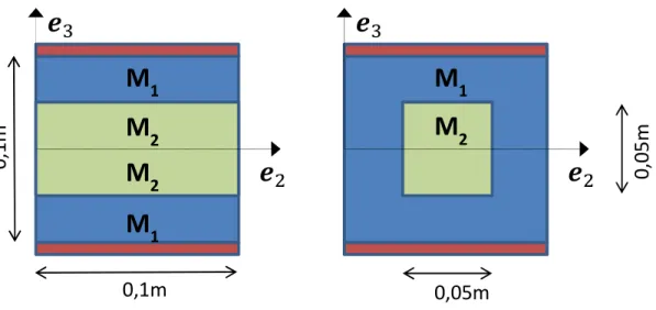
Following the validation test used by Nguyen, we consider the case of a two phases laminate plate for which a closed form solution exists (see [28]). The unit-cell Ω represented on Figure 1, is symmetric so that the coupling tensor 𝐵 vanishes. The volume fractions of phases are equal (50%), and their elastic properties (Young modulus, Poisson coefficient) are respectively (46GPa, 0.3) and (10GPa, 0.3) for phases 1 and 2. According to [28], the spatial resolution used for the simulations are 2n_x2n_{(x1) voxels (the code is 3D) for the unit cell Ω and two additional layers enlarge the unit-cell to}

simulate traction-free boundary condition in Ω∗ _{(see section 2). The non-null components (𝐸 , 𝜒 )}

of 𝐸 and 𝜒 defines the two applied loadings: (1,0) for the tensile loading and (0,1) for the bending loading. They directly allow to evaluate 𝐴 = 𝑁 ⁄𝐸 and 𝐷 = 𝑀 ⁄𝜒 . The corresponding loadings applied to the enlarged unit-cell Ω∗ _are:

𝐸∗ ₌ 𝟎_{𝟎 𝑬}𝟎 0 𝟐𝟐 0 0 0 0 , 𝜒∗ _{= 0 (tension)} 𝐸∗ _{= 0, 𝜒}∗ ₌ 𝟎_{𝟎 𝜒}𝟎 0 𝟐𝟐 0 0 0 0 (bending) ₍₂₃₎

The choice made for the reference material’s Lamé coefficients (𝜆 , 𝜇 ) is 𝜆 = (𝜆 + 𝜆 )/2 with 𝜆 = 0 (for the void layers) and 𝜇 = (𝜇 + 𝜇 )/2 with 𝜇 = 0 (for the void layers). adjusted to obtain a Poisson coefficient 𝜐 = 0.3, the Poisson coefficient common to both phases.

Figure 1 : Description of the two unit-cells used in simulations of heterogeneous plates: laminate plate (left) and composite plate with cylinder (square base) inclusions (right). In orange are represented the additional void layers used in the present simulations.

For the tensile loading, the algorithm reaches convergence after 6 iterations with a convergence criterion on the local equilibrium of 10-15 _{far below the threshold of 10}-4 _{used for the simulation. It}

seems that the solver reaches the exact solution, up to the double precision round-off error.

Actually, the exact solution being constant per layer, it can be observed that the FFT-based method is able to find it if the discretization grid is parallel to the layers. From the macroscopic point of view, Table 1 gathers the comparison with analytical results and numerical results from [28]. The

comparison with analytical result is exact up to the 8th _{digit. The comparison with [28] is perfect up to}

the number of available digits. However, the converged value is obtained after 10 iterations to converge on a macroscopic criterion (10-4 _{on the average energy between two iterations), compared}

to 6 for this study on a more stringent criterion (local equilibrium). Finally, as the solution is constant per layer, it does not depend on the mesh resolution and exactly the same result is obtained with a resolution 4x4 (i.e. with one voxel per layer in the thickness).

Resolution Analytical This work [28] 8x8 3.07692307 3.07692303 3.077 4x4 3.07692307 3.07692303

Table 1 : Axial stiffness 𝐴 obtained for the laminate case: comparison between analytical results and two FFT-based methods

For the bending loading, the algorithm reaches convergence after 15 iterations with, once again, a convergence criterion on the local equilibrium of 10-10 _{far below the threshold of 10}-4_{. As mentioned}

earlier, the method is able to find perfectly equilibrated layered stress fields (up to the precision round off and as soon as the layer are parallel to the discretization grid). However, In the case of bending, the stress field is not constant per phase so that the stress field and consequently the resultant ‘stress’ tensor 𝑀, depends on the mesh size. Table 2 compares the analytical results with the numerical results in [28] and this study, for different spatial resolutions. Both results are in excellent agreement with the analytical case and the error becomes very low as soon as resolution reaches 32x32. For resolution 16x16, results are still in good agreement (relative error ~0.26%) and Nguyen’s method provides a similar precision (a bit less but with a lower, i.e. 10, number of

𝒆

𝒆

M

M

M

M

𝒆

𝒆

M

M

0,

1m

0,1m

0,05m

0,

05

m

iterations). looks better in that case. On the other hand, it required 10 iterations to reach convergence (on a macroscopic criterion), compared to a single iteration in this study.

Resolution Analytical (GPa/m) This study (rel. error) [28] (rel. error) 16x16 0.0038003663 0.0037903502 (26e-4) 0.00382 (52e-4) 32x32 0.0038003663 0.0037978623 (7e-4) 0.003805 (13e-4) 64x64 0.0038003663 0.0037997403 (2e-4) 0.003802 (5e-4) 128x128 0.0038003663 0.0038002098 (4e-5) 256x256 0.0038003663 0.0038003272 (1e-5) 512x512 0.0038003663 0.0038003566 (2e-6) 1024x1024 0.0038003663 0.0038003638 (7e-7)

Table 2 : Bending stiffness 𝐷 obtained for the laminate case: comparison between analytical results and two FFT-based methods

An additional example demonstrating that our FFT-based approach converges towards analytical results can be found in Annex B with a Poisson ratio of 10-4 _{(close to 0).}

To conclude, the minor modification applied to our general FFT-based solver, allows reproducing the analytical solution obtained for a laminate plate, at least as precisely and as efficiently as an FFT-based solver dedicated to the homogenization of plates.

3.1.3 : Plate with periodic fibers [28]

This second validation test proposed in [28] considers a panel with a periodic distribution of

parallelepiped fibers. Figure 1 describes the periodic unit-cell. The matrix and the inclusion have the same Poisson ratio (0.3), and the Young moduli of inclusion / matrix (in GPa) are (0/1), (10/1) and (1/1000). The AMITEX_FFTP code being able to apply whether the average stress or the average strain 𝐸∗ _{for each of the six components, applying a null average stress for the components 33, 13}

and 23, was found to reduce the number of iterations at convergence of about 30% for the tensile loading. Hence, the loading used in this case is identical to the loading introduced for the laminate case in equation (23), except for these three components, now set to null stress instead of null strain. The bending loading remains unchanged. The choice made for Lamé coefficients follows the same rule as proposed in the laminate case. The spatial resolution used for the simulations are 2n_x2n_(x1)

voxels (the code is 3D) for the unit cell Ω and two additional layers enlarge the unit-cell to simulate traction-free boundary condition in Ω∗ _{(see section 2).}

All the simulations reported in [28] have been reproduced and all the results are gathered in tables of annex C, in which the membrane stiffness 𝐴 , bending stiffness 𝐷 and number of iterations are given as a function of the spatial resolution for the three elastic contrasts. The convergence criterion being very different between AMITEX_FFTP and [28], the comparison between iteration numbers at convergence is not significant. Hence, the evaluation of strain energy has been implemented in AMITEX_FFTP and the relative difference between two iterations is evaluated as a post-treatment to determine the number of iterations at convergence if using this criterion with a threshold of 10-4

(used in [28]).

If not useful to discuss all the tables one by one, their analysis allows drawing a few main conclusions. First, even for the coarsest resolution (16x16), with relative errors below 1%, results

obtained with both FFT-based methods are very close to the reference solution obtained from finite element simulations in [28]. Second, if the relative error decreases monotonously with Nguyen’s method, the decrease is less monotonous with our approach and, in addition, the relative error do not seem to decrease below 0.1% for the bending loading cases. If this question could be further investigated, in practice a relative error of 0.1% is yet below the accuracy required by many applications. Second, the results are also quite comparable with [28]’s with a relative error that decreases quite monotonously as a function of the spatial resolution. Third, the number of iterations obtained with our approach (associated to a field equilibrium criterion) remains reasonable with values comprised between 20 and 76. It is a bit lower for bending loadings than for tensile loadings, whereas the type of loading has no influence on [28]’s results. Finally, when post-treating our results with the strain energy based criterion, the number of iterations at convergence are rather similar to [28]’s results., a bit higher for tensile loadings and a bit lower for bending.

Finally, additional results obtained with realistic material properties are also given in Annex C. The material corresponds to a glass fiber/epoxy composite with the couple (Young modulus, Poisson coefficient) being respectively (73.1GPa, 0.22) and (3.45GPa, 0.35) for glass and matrix. The elastic contrast is around 20 and here, the Poisson coefficients are different. The homogenized coefficient exhibit a monotonous convergence and the number of iteration of the algorithm is a bit higher than the previous ones but remains below 100.

To conclude, the minor modification applied to our general FFT-based solver, allows reproducing the numerical results obtained for a matrix/inclusion plate, almost as precisely and as efficiently as a solver dedicated to the homogenization of plates.

3.2 : Homogenization of beams

If the extension of the approach proposed for plates in [28] to the homogenization of beams is not straightforward especially with arbitrary cross-sections, it is direct with our approach. After a description of the method proposed for the homogenization of beams, it is applied to different loadings with various geometries and elastic contrasts. As uniaxial tension is quite straightforward and has already been applied in previous studies [10], the paper focuses on bending and torsion loadings.

This section considers two different beams with a square and a disk cross-section. In the first case the discretization is conform to the geometry while it is not in the second case. Cubic inclusions, with conform discretization are considered in both cases, so that the effect of a conforming discretization is limited to the shape of the cross-section which is of a prime interest in the present context.

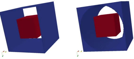
Figure 2 : Rendering of the two unit-cells: on the left with a square cross-section, on the right with a disk cross-section. The cubic inclusion is in red, the added void volume is in blue and the matrix in transparency.

Figure 2 represents the geometry of the unit-cell with a cube diameter of 50mm, a unit-cell length of 100mm, a square and disk diameter of 100mm for the cross-section. Void volumes in blue

complement the unit-cells Ω, with a minimal thickness of two voxels, to form the enlarged unit-cells Ω∗. The center of the inclusion lies on the axis of the unit-cells. The spatial resolutions, defined by the number of voxels on 100mm, are 40, 80 and 160 (so that the unit-cells are 40x44x44, 80x84x84 and 160x164x164). With these resolutions, the discretization of the inclusion is conform to its geometry.

The Young modulus of the matrix is 10MPa with a Poisson coefficient of 0.3 and three elastic behaviors are considered for the inclusion: the matrix behavior, so that the beam is homogeneous, a void behavior leading to an infinite contrast and a behavior stiffer than the matrix with a high contrast 1000.

In addition, the use of composite voxels [17] [22] [21] [8] is tested to improve the description of the geometry when using a non-conforming discretization, as observed with the disk cross-section. The behavior of the composite voxels, crossed by the interface between the matrix and the additional void volume, follows a homogenization rule. Among the three classical rules, the Reuss and laminate homogenization rules are not well-suited with void behavior: the first one simply replaces the voxel by a void voxel and the second leads to an infinitely anisotropic behavior which generates

convergence issues in the FFT-based algorithm (observed in torsion loading). In addition, the Voigt homogenization rule, which assumes a homogeneous strain over the phases, is extremely simple to implement, even with non-linear behaviors. Voigt is used in the following. For the sake of simplicity, an approximate definition of volume fractions is used and reported in annex D.

The choice made for the reference material’s Lamé coefficients (𝜆 , 𝜇 ) is 𝑋 = (𝑋 + 𝑋 )/2, with 𝑋 equal to 𝜆 or 𝜇. Note that here, min and max are evaluated over the beam material, excluding the additional void volume in Ω∗_{: for contrasts 0 and 1000, the difference are null or very small, and}

for contrast 1, the reference material corresponds to the behavior of the homogeneous beam.

3.2.1.1 : General settings

The unit-cell Ω with an arbitrary cross-section is periodic in direction 𝒆𝟏. and, for numerical

resolution purpose, is enlarged by additional voxels of null stiffness to form a parallelepiped unit-cell Ω∗_{, as shown on the two examples on Figure 2. Assuming an applied strain field consistent with}

the Bernoulli modeling for beams, the problem to solve reads:

⎩ ⎪ ⎨ ⎪ ⎧𝒅𝒊𝒗(𝜎) = 0_{𝜎 = 𝑐: 𝜀} 𝜀 = 𝐸 + 𝜒 𝑥 + 𝜒 𝑥 + (∇𝒖) 𝒖 periodic on ∂ Ω 𝜎. 𝒏 antiperiodic on ∂ Ω 𝜎. 𝒏 = 0 on ∂ Ω (24)

Where ∂ Ω denotes the two faces of normal direction 𝒆𝟏, submitted to periodic boundary

conditions, and ∂ Ω the external contour of the beam submitted to a traction-free boundary condition. The macroscopic applied strain is limited to components in bold in equation (25). The component 𝐸 prescribes a tensile loading, the components 𝐺 and 𝐺 prescribe two bending loadings respectively, and 𝛼 = 𝐺 = −𝐺 prescribes the torsion loading. According to the arguments proposed in Annex A based on the vanishing components of 𝐸 and 𝐺 imposed by the periodicity condition in direction 1, only the 11 component of the 𝐸, 𝜒 and 𝜒 can be prescribed. However, the component 𝛼 = 𝐺 = −𝐺 was successfully prescribed for the torsion loading in the simulations below. Additional arguments to explain this point are still under investigation. As mentioned for plates in section 3.1.1, due to mechanical coupling between directions, the other components are not prescribed but do not systematically vanish (the simplest example being the Poisson effect). 𝐸 = 𝑬𝟏𝟏 𝐸 𝐸 𝐸 𝐸 𝐸 𝐸 𝐸 𝐸 ; 𝜒 = 𝑮𝟏𝟏𝟑 −𝛼 𝐺 −𝛼 𝐺 𝐺 𝐺 𝐺 𝐺 and 𝜒 = 𝑮𝟏𝟏𝟐 𝐺 𝛼 𝐺 𝐺 𝐺 𝛼 𝐺 𝐺 ₍₂₅₎

3.2.1.2 : FFT-based resolution on an enlarged unit-cell Ω∗

In order to satisfy the traction-free boundary condition, the full periodic problem is solved on the enlarged unit-cell Ω∗ _{with a void volume surrounding Ω in order to fulfil the traction free boundary}

condition on ∂ Ω. Due to the added void layers, the out of plane components prescribed to Ω∗ _are

the same as prescribed to Ω (in bold) but the in plane components can be chosen arbitrarily. They are set to 0. 𝐸∗ ₌ 𝑬₀𝟏𝟏 0₀ 0₀ 0 0 0 ; 𝜒∗ ₌ 𝑮_−𝛼𝟏𝟏𝟑 −𝛼₀ 0₀ 0 0 0 and 𝜒∗₌ 𝑮𝟏𝟏𝟐₀ 0₀ 𝛼₀ 𝛼 0 0 (26) The discussion on prescribed components and components that can be chosen arbitrarily is similar to the discussion proposed for plates. It has been checked on a homogeneous beam with 𝐸∗ _{= 1 and}

𝐺∗ = 𝐺∗ = 1, that the strain field is homogeneous with an average on Ω corresponding to 𝐸 = 1, 𝐸 = 𝐸 = −𝜈𝐸 (and null shear strain components). The arbitrary choice of the components 𝐺∗ is general (Annex A) and was already checked in section 2.4. As mentioned before, it has been

verified that the torsion loading applied to Ω∗ _{is actually prescribed on Ω. So the torsion loading can}

be applied in our numerical experiments (with numerical results consistent with analytical results for the homogenous beam), but the reason of this has still to be clarified as it is not expected from arguments given in Annex A.

In order to use the method proposed in section 2 to account for linearly varying applied strain, the strain gradient components imposed in equation (26) have to satisfy the constraints established in the general case (set of equations ). In the present case, the torsion component 𝛼 = 𝐺 = −𝐺 remains unconstrained and two constraints apply to 𝐺 and 𝐺 components:

𝜆 (𝐺 + 𝐺∗ + 𝐺∗ ) + 2𝜇 𝐺∗ _{= 0}

𝜆 (𝐺 + 𝐺∗ _{+ 𝐺}∗ _{) + 2𝜇 𝐺}∗ _{= 0}

These constraints allow proposing two elementary bending beam loadings, governed by the components 𝐺 and 𝐺 applied to Ω, as follows:

⎩ ⎨ ⎧𝐺_𝐺∗ imposed_{= 𝛽𝐺}∗ 𝐺∗ = − 𝜆 𝜆 (1 + 𝛽) + 2𝜇 𝐺 ⎩ ⎨ ⎧𝐺 ∗ _{= 𝛽𝐺}∗ 𝐺 imposed 𝐺∗ = − 𝜆 𝜆 (1 + 𝛽) + 2𝜇 𝐺

These two loadings are very similar to the bending plate loadings (one is identical with 𝛽 = 0) given in equation . As mentioned in the case of plates, because of the void volume surrounding Ω in Ω∗_,

the volume Ω is free to deform in the directions 𝒆𝟐 and 𝒆𝟑, so that the values of 𝐺 and 𝐺 (with

(𝑖, 𝑗) ∈ {1,2} ) evaluated over Ω can be different from their corresponding values 𝐺∗ over the enlarged cell Ω∗_{. The same consideration holds for the null components 22, 33 and 23 of 𝐸}∗_{. The}

parameter 𝛽 is set to 1 in the present paper. 3.2.1.3 : Homogenization of beams

Once, the problem solved at the micro-scale (on the heterogeneous unit-cell), the last step consists in defining appropriate spatial averages for the macroscopic quantities used for modeling beams. Classically, integrations of the traction vector (𝜎. 𝒆𝟏) over the cross-section provide the macroscopic

force 𝑵 (expressed in N) and moments 𝑴 (in N.m) as follows:

𝑵 = 𝜎. 𝒆𝟏𝑑𝑆 = 𝜎 𝜎 𝜎 𝑑𝑆 𝑴 = 0 𝑥 𝑥 ∧ (𝜎. 𝒆𝟏)𝑑𝑆 = 𝜎 𝑥 − 𝜎 𝑥 𝜎 𝑥 −𝜎 𝑥 𝑑𝑆 (27)

The 𝑁 component of the force vector is the axial force and the other components are shear forces. The 𝑀 component of the moment vector is the torsion moment and the other components are bending moments. For homogenization purpose, these quantities evaluated on a cross section are averaged over the 𝒆𝟏 direction of the unit-cell Ω so that they can be evaluated from volume

𝑵 =1 𝑙 𝜎. 𝒆𝟏𝑑𝑆 𝑑𝑥 = 1 𝑙 𝜎. 𝒆𝟏𝑑𝑉 𝑴 =1 𝑙 0 𝑥 𝑥 ∧ (𝜎. 𝒆𝟏)𝑑𝑆 𝑑𝑥 = 1 𝑙 0 𝑥 𝑥 ∧ (𝜎. 𝒆𝟏)𝑑𝑉 (28)

Using the axial periodicity of 𝒖 and the equilibrium condition (∫ _{( )}𝜎 𝑑𝑆= ∫ _{( )}𝜎 𝑑𝑆= 0, for all longitudinal sections 𝑆 (𝑥 ) and 𝑆 (𝑥 )), it can be demonstrated that the average of the microscopic energy is equal to the macroscopic energy. In the case of beams, the energy linear density is considered and the so-called macro-homogeneity condition of Hill-Mandel reads:

1 𝑙 𝜎: 𝜀𝑑𝑉 = 1 𝑙 𝜎: (𝐸 + 𝜒 𝑥 + 𝜒 𝑥 + 𝜀̃)𝑑𝑉 = 𝑁 : 𝐸 + 𝑀 : 𝐺 − 𝑀 : 𝐺 + 2𝑀 : 𝛼 (29)

The different terms are respectively associated to the uniaxial, the two bendings and the torsion loadings. The minus sign of the third term comes from the minus sign of 𝑀 in equation (27).

Finally, the homogenized elastic behavior relates the kinematic quantities 𝑼 = (𝐸 , 𝛼, 𝐺 , 𝐺 ) to the forces and moments 𝑭 = (𝑁 , 𝑀 , 𝑀 , 𝑀 ) with a linear relationship:

𝑭 = 𝐾: 𝑼 ₍₃₀₎

As mentioned for plates, the Hill-Mandel condition allows using indifferently the energetic or the mechanical approach. The last one is used in the following: a single kinematic loading is applied and the stress field is post-treated to evaluate forces and moments and identify the stiffness components of 𝐾.

3.2.2 : Beam bending

The bending loading is applied to the unit-cell Ω∗ _{with 𝐺}∗ _{= 𝐺 . Components 𝐺}∗ _{and 𝐺}∗

arbitrarily set to 0 in equation (26) are now set to - 𝜈𝐺∗ _{. Even if components 222 and 332 are not}

prescribed to the unit-cell Ω, they provide a better initialization of the strain field and reduce the number of iterations at convergence. For the homogeneous strain loading, three different

propositions have been tested: all the average strain components equal to 0, all the average stress components equal to 0, average strain components (1𝑗) , , and average stress components

(𝑖𝑗) , , equal to zero. All the propositions provide the same bending moment 𝑀 (up to a

relative difference of ~10-4_{) and none of them outperforms the others regarding the number of}

iterations at convergence. Results below are presented with all the average strain components equal to 0.

In practice, 𝐺 is set to 1 in the simulations so that the bending moment is directly the bending stiffness.

The case of a homogeneous beam is interesting, at first as a validation case for which the analytical solution is known, but also to focus on the question of the non-conforming discretization of the beam (for the disk cross-section) and the potential interest of using composite voxels (with Voigt homogenization rule in that case). This specific case is also interesting because the initialization of the strain field in the FFT-based algorithm directly provides the solution of the problem and

convergence should achieve at the first iterate. Actually, the initial strain field is a null homogeneous strain field added to a linearly varying strain field associated to 𝐺 and 𝐺∗ _{= 𝐺}∗ _{= −𝜈𝐺 (see}

introduction of 3.2.2) and 𝐺∗ _{= 𝐺}∗ _{= −}

( )𝐺 (see equation ). Hence, the initialization of

the strain field imposes 𝜀 = 𝜀 = 𝜀 = 0 for shear strains, 𝜀 = 𝐺 𝑥 for the axial strain and 𝜀 = 𝜀 = −𝜈𝜀 for the transverse strains. This strain field initialized on the whole unit-cell Ω∗

also applies on the sub-volume Ω so that, if the Poisson coefficient of the reference medium 𝜐 is equal to the Poisson coefficient of the beam material 𝜐, the initial strain field it is directly the solution of the bending problem. As a validation part, the implementation in the AMITEX_FFTP code confirms this property : convergence is reached at the first iterate.

The bending moments derived from the Euler-Bernoulli beam theory are:

𝑀 = 𝐸𝜋𝐷

64 𝐺 (disk cross section) and 𝑀 = 𝐸 𝐷

12𝐺 (square cross section) (31)

Figure 3 represents the evolution of the relative error of the bending moments as a function of the spatial resolution. For the square cross-section, with a conform discretization the error is very low even for the lowest resolution (6.10-4_{) and decreases monotonously to around 10}-5_{. On the contrary,}

for the disk cross section, the error is much higher and decreases with the spatial resolution from 0.01 to reach a value around 1.10-4 _{for the highest resolution. This difference clearly exhibits, on the}

macroscopic property, the difference between conforming and non-conforming discretization. For the square cross-section, the error is purely associated to the numerical integration of a quadratic field (𝜎 𝑥 ) on a rectilinear grid, whereas for the disk cross-section, an additional and predominant error due to the non-conforming discretization of the cross-section is added. In that case, the composite voxels demonstrate their efficiency to improve the results: the relative error is between 5 and 100 times lower than without composite voxels. As expected, the factor for resolution 40 (factor 37) is higher than for resolution 160 (factor 5). The factor 100 for resolution 80 was not really expected. It could be the sign of an optimum resolution for the efficiency of composite voxels. The question is beyond the scope of the paper. is 3.10-4 _{for the lowest resolution and stabilizes around}

10-5_{. From the stress field point of view, as observed on Figure 4, the composite voxels only modify}

the stress within the voxels crossed by the interface. In that case, their effect is purely local (it will be different for torsion loading).

Figure 3 : Evolution of the relative error on the evaluation of the bending moment as a function of the spatial resolution, for homogeneous beams with square and disk cross-sections, and with the use of composite voxels for disk cross-sections.

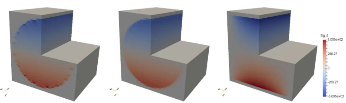
Figure 4 : Axial stress field obtained for the disk cross-section with (right) and without (left) composite voxels, for the lowest spatial resolution (40) (for visualization purpose a quarter of the unit-cell is removed) and an homogeneous beam.

3.2.2.2 : Heterogeneous beam bending

Figure 5 (right) represents the evolution of the bending moments (or bending stiffness as 𝐺 = 1) for the three different elastic contrasts. It is worth noting that in spite of high contrasts, the evolution of the bending stiffness is moderate. Different observations can explain this result. At first, the volume fraction of inclusions is not so high (12.5% and 15.9%, respectively for the square and disk cross-sections). Then, and probably more importantly, the inclusions are located at the center of the beam, which is the less stressed region of the beam. It is also noticeable that the difference on the moments between square and disk cross-sections is almost independent of the contrast (respectively (3.42, 3.42, 3.45)x107 _{for the contrasts (0,1,1000)). In other words, the stiffening (or softening)}

induced by these stiff (or soft) inclusions, with respect to the homogeneous beam, corresponds to an additional positive (or negative) bending stiffness that is rather independent of the beam cross-section.

Regarding the convergence analysis w.r.t. the spatial resolution, Figure 5 (left) displays the evolution of the bending moments, normalized by their converged value (obtained for resolution 160). The

same conclusions as obtained for the homogeneous beam still hold for heterogeneous beams: convergence is very fast for the square cross-section, unlike the case of the disk cross-section without composite voxels, and using composite voxels significantly improves the convergence. The effect of the contrast, moderate on the converged values of the moments (see Figure 5 (right)), is also quite moderate on the convergence curves (see Figure 5 (left)).

Regarding the convergence analysis of the FFT-based algorithm (in our case, a fixed-point algorithm combined with a convergence acceleration procedure), presented on Table 3, four main conclusions can be drawn. First, the convergence is very efficient for void inclusions. Second, stiff inclusions drastically deteriorate the convergence. Note that, in that case, the unit-cell Ω∗ _{exhibits two types of}

large elastic contrast: between the matrix and the infinitely soft voids and between the matrix and the 1000 times stiffer inclusions. Such high and opposite contrasts are not really well suited for FFT-based methods. However, convergence is achieved and the number of iteration remains reasonable. Third, the use of composite voxels deteriorates the convergence by a factor of around 2. Fourth, for the square cross-section, increasing the spatial resolution deteriorates the convergence, but it tends to stabilize in the worst case with the contrast of 1000. The understanding of these last two

unexpected results is still under investigation.

The analysis of the local stress fields focuses on the simulations with an elastic contrast of 1000 that induces the highest contribution to the bending stiffness (compared to the homogeneous beam, see Figure 5 (right)) and exhibits the worst algorithm convergence (see Table 3). The worse convergence of the algorithm is probably to be correlated with the spurious oscillations arising in and around the stiff inclusion. Comparing the disk and square cross-sections, the stress fields in and around the inclusion are almost identical, independent of the cross-section. This is consistent with the previous observation, at the macroscopic scale, of an additional contribution to the bending stiffness independent of the cross-section. Finally, comparing the disk cross-section with and without composite voxels, the conclusion reported for homogeneous beam still holds in the heterogeneous cases: they essentially affect the voxels crossed by the interface, keeping unchanged the rest of the volume (it will be different for torsion loading).

Figure 5 : Evolution of the bending moments (normalized by their converged values obtained for the highest resolution) as a function of the spatial resolution; with solid, dotted and dashed lines respectively for contrasts 1, 0 and 1000 (left). Evolution of the converged values of the moments (obtained for the highest resolution) as a function of the contrast (the arrows symbolize null contrasts in log axis) (right). Note that ‘disk’ and ‘disk+composite voxels’ symbols are superimposed, confirming that the moments obtained with the ‘disk’ (without composite voxel) at resolution 160 are converged values.

Figure 6 : Axial stress field obtained for the square cross-section (right), and the disk cross-section with (left) and without (middle) composite voxels, for the lowest spatial resolution (40) and a contrast of 1000 for the inclusion (for visualization purpose a quarter of the unit-cell is removed). Bottom figures are zooms on the inclusion with an appropriate color bar.

Resolution Square Disk Disk with Composite Voxel C=0 C=1 C=1000 C=0 C=1 C=1000 C=0 C=1 C=1000 40 16 1 456 16 1 423 25 1 699 80 21 1 600 15 1 336 24 1 666 160 28 1 759 15 1 366 24 1 763

Table 3 : Number of iteration at convergence for the different beams, contrasts, resolutions and use of composite voxels (bending loading case)