Dynamic state-space estimation of the hemodynamic response with Near-Infrared Spectroscopy

Dynamic state-space estimation of the

hemodynamic response with Near-Infrared

Spectroscopy

by

Louis Gagnon

B.S. Engineering Physics, M.S. Biomedical

Ecole Polytechnique de Montreal

Engineerin

MASSACHUSETTS INSTITUTE

OF TECI-NOLOGY

SEP 2 7 2011

LiBPARIES

ARCHIVES

Submitted to the Department of Electrical Engineering and Computer

Science

in partial fulfillment of the requirements for the degree of

Master of Science in Electrical Engineering and Computer Science

at the

MASSACHUSETTS INSTITUTE OF TECHNOLOGY

September 2011

©

Massachusetts Institute of Technology 2011. All rights reserved.

Author...

..

Department of

_{El ctrica Engineering and Computer Science}

.

.

..

,.

- %

...

. . . . .

/

September 7, 2011

C ertified by ... . . .... ... ...

David A. Boas

Associate Professor of Radiology

Thesis Supervisor

Accepted by ...

...

Leslie A. Kolodziejski

Dynamic state-space estimation of the hemodynamic

response with Near-Infrared Spectroscopy

by

Louis Gagnon

B.S.

Engineering Physics, M.S. Biomedical Engineering

Ecole Polytechnique de Montreal

Submitted to the Department of Electrical Engineering and Computer Science on September 7, 2011, in partial fulfillment of the

requirements for the degree of

Master of Science in Electrical Engineering and Computer Science

Abstract

Near-Infrared Spectroscopy (NIRS) allows the recovery of the hemodynamic response associated with evoked brain activity. The signal is contaminated with systemic phys-iological interference which occurs in the superficial layers of the head as well as in the brain tissue. The back-reflection geometry of the measurement makes the DOI signal strongly contaminated by systemic interference occurring in the superficial layers. A recent development has been the use of signals from small source-detector separa-tion (1 cm) optodes as regressors. Since those addisepara-tional measurements are mainly sensitive to superficial layers in adult humans, they help in removing the systemic interference present in longer separation measurements (3 cm). Encouraged by those findings, we developed a dynamic estimation procedure to remove global interference using small optode separations and to estimate simultaneously the hemodynamic re-sponse. The algorithm was tested by recovering a simulated synthetic hemodynamic response added over baseline DOI data acquired from 6 human subjects at rest. The performance of the algorithm was quantified by the Pearson R2 _{coefficient and the}

mean square error (MSE) between the recovered and the simulated hemodynamic responses. Our dynamic estimator was also compared with a static estimator and the traditional adaptive filtering method. We observed a significant improvement (two-tailed paired t-test, p < 0.05) in both HbO and HbR recovery using our Kalman

filter dynamic estimator compared to the traditional adaptive filter, the static estima-tor and the standard GLM technique. We then show that the systemic interference occurring in the superficial layers of the human head is inhomogeneous across the sur-face of the scalp. As a result, the improvement obtained by using a short separation optode decreases as the relative distance between the short and the long measurement

is increased. NIRS data was acquired on 6 human subjects both at rest and during a motor task consisting of finger tapping. The effect of distance between the short and the long channel was first quantified by recovering a synthetic hemodynamic response added over the resting-state data. The effect was also observed in the functional data collected during the finger tapping task. Together, these results suggest that the short separation measurement must be located as close as 1.5 cm from the standard NIRS channel in order to provide an improvement which is of practical use. In this case, the improvement in Contrast-to-Noise Ratio (CNR) compared to a standard GLM procedure without using any small separation optode reached 50% for HbO and 100% for HbR. Using small separations located farther than 2 cm away resulted in mild or negligible improvements only.

Thesis Supervisor: David A. Boas

Acknowledgments

I first want to thank David, my advisor, who supervised my research from the

begin-ning and without whom this work would have not been possible. I received encour-agements from a lot of peoples during the course of this work. This includes all my colleagues at the Photon Migration Imaging Lab (now The Optics Division), Bruce Rosen, Jonathan Polimeni, Jean Chen and Doug Greve at the Martinos Center, and

Al Oppenheim, Georges Verghese, Mehmet Toner and Elfar Adalsteinsson at MIT.

Thanks a lot!

I want to thank my collaborators Sol Diamond, Emery Brown, Patrick Purdon, Lino

Becerra and Dana Brooks for interesting discussion about state-space modeling and the Kalman filter. I am also grateful to Drs. Evgeniya Kirilina, Yunjie Tong and Blaise deB. Frederick for fruitful discussions about cerebrovascular physiology. Finally, I want to acknowledge financial support from the Fonds Quebecois sur la Nature et les Technologies (FQRNT), the IDEA-squared program at MIT as well as from the Canadian Center for Mathematical Research. My research was also supported by NIH grants P41-RR14075 and RO1-EB006385.

Contents

1 Introduction

2 State-space modeling for NIRS

2.1 M ethods . . . . 2.1.1 Experimental data . . . . 2.1.2 Synthetic hemodynamic response

2.1.3 Signal modeling . . . . 2.1.4 Standard General Linear Model

2.1.5 Adaptive filtering . . . .

2.1.6 Static estimator . . . .

2.1.7 Kalman filter estimator . . . .

2.1.8 Statistical analysis . . . . 2.2 R esults . . . .

2.3 _{Discussion . . . .} 2.3.1 Simultaneous filtering and estimation

2.3.2 Dynamic versus static estimation

2.3.3 HbO versus HbR . . . .

2.3.4 Impact of initial correlation . . .

2.3.5 Technical notes . .

2.3.6 Future directions . . . . 2.4 Summary ...

2.5 Appendix: Design matrix . . . .

3 Impact of the short channel location 3.1 M ethods . . . . 3.1.1 Experimental data . . 3.1.2 Data processing . . . . 3.1.3 Simulations . . . . 3.1.4 Functional data . . . . 3.2 Results . . . . 3.2.1 Baseline correlation . . 3.2.2 Simulation results . . .

3.2.3 Functional data results

3.3 Discussion . . . .

3.3.1 Systemic interference measured by NIRS is inhomogeneous across

. . . . 5 8 . 35 . 36 . . . . . . . . . . . . . . . . . 3 7 . . . . . . . . 39 . . . . . 39 . . . . . . . . 43 . . . . . . . . . . 49 . . . . . . . . . . . . . . . . . . . . . . 5 2 . . . . 5 2 . . . . 5 4 . . . . 5 8 the scalp

3.3.2 Impact on the short separation method . . . . 64

3.3.3 Future studies . . . . 66

3.4 Sum m ary . . . . 66

List of Figures

1-1 Sensitivity profile of a given source-detector pair in NIRS . . .

1-2 Illustration of the short separation regression method in NIRS

2-1 O ptical probe . . . . 2-2 Tem poral basis set . . . .

2-3 Time courses of the recovered hemodynamic responses . . . .

2-4 Summary of the Pearson R2 statistics . . . .

2-5 Summary of the MSE statistics . .

3-1 Multiple short separation optical probe

3-2 Functional protocol

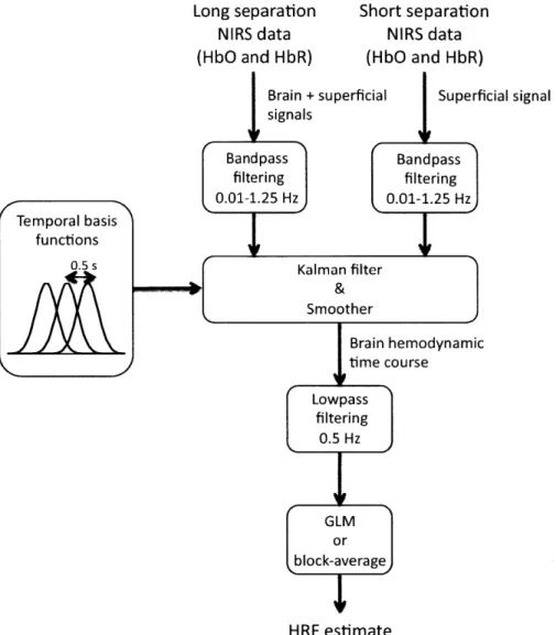
3-3 State-space analysis

3-4 Baseline correlation

3-5 Summary R2 results

3-6 Summary MSE results

3-7 Summary CNR results

. . . . . . . . . . . . 33

. . . . . . . . . . . . . . 4 5

. . . . . . . . . . . . . . . 5 5

3-8 Summary in vivo finger tapping . . . . 59

3-9 Correlation 0.01-0.2 Hz . . . . 61

3-10 Correlation 0.2-0.5 Hz . . . . 62

List of Tables

Chapter 1

Introduction

Diffuse optical imaging (DOI) is an experimental technique that uses near-infrared spectroscopy (NIRS) to image biological tissue [48, 37, 13, 19, 20]. The dominant chro-mophores in this spectrum are the two forms of hemoglobin: oxygenated hemoglobin

(HbO) and reduced hemoglobin (HbR). In the past 15 years, this technique has been

used for the noninvasive measurement of the hemodynamic changes associated with evoked brain activity [48, 20].

Compared with other existing functional imaging methods e.g., functional Mag-netic Resonance Imaging (fMRI), Positron Emission Tomography (PET), Electroen-cephalography (EEG), and MagnetoenElectroen-cephalography (MEG), the advantages of DOI for studying brain function include good temporal resolution of the hemodynamic re-sponse, measurement of both HbO and HbR, nonionizing radiation, portability, and low cost. Disadvantages include modest spatial resolution and limited penetration depth.

The sensitivity of NIRS to evoked brain activity is also reduced by systemic physio-logical interference arising from cardiac activity, respiration, and other homeostatic processes [36, 46, 38, 8]. These sources of interference are called global interference or systemic interference. Part of the interference occurs both in the superficial layers of

the head (scalp and skull) and in the brain tissue itself. However, the back-reflection geometry of the measurement makes NIRS significantly more sensitive to the super-ficial layers as illustrated in Fig. 1-1. As such, the NIRS signal is often dominated by systemic interference occurring in the skin and the skull.

Figure 1-1: Sensitivity profile of a given source-detector pair in NIRS.

Different methods have been used in the literature to remove the systemic interference from DOI measurements. Low pass filtering is widely used in the literature, as it is

highly effective at removing cardiac oscillations [9, 29]. However, there is a

signifi-cant overlap between the frequency spectrum of the hemodynamic response to brain activity and the spectrum of other physiological variations such as respiration, sponta-neous low frequency oscillations and very low frequency oscillations. Frequency-based removal of these sources of interference can therefore result in large distortion and inaccurate timing for the recovered brain activity signal. As such, more powerful methods for global noise reduction have been developed. These include adaptive av-erage waveform subtraction [15], subtraction of another NIRS source-detector (SD) channel performed over a non-activated region of the brain [9], principal component analysis [50, 10] and finally wavelet filtering [33, 35, 28, 34].

A recent development for removing global interference from NIRS measurements is

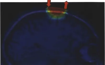
sensitive to superficial layers only [42, 52, 53, 51, 47, 49, 16]. This method is illustrated in Fig. 1-2. Making the assumption that the signal collected in the superficial layers is

Figure 1-2: Illustration of the short separation regression method in NIRS. (Figure taken from Zhang et al [52].)

dominated by systemic physiology which is also dominant in the longer SD separation NIRS channel, those additional measurements can be used as regressors to filter systemic interference from the longer SD separations. Saager et al [41] used additional optodes and a linear minimum mean square estimator (LMMSE) to partially remove the systemic interference in the signal. In a second step, the evoked hemodynamic response was estimated using a traditional block-average method over the different trials. The algorithm was further refined by Zhang et al [52, 53, 51] to consider the non-stationary behavior of the systemic interference. They used an adaptive filtering technique together with additional small separation measurements to filter the systemic interference from the raw signal and then performed the block-average technique to estimate the hemodynamic response in a second step.

Although these methods greatly reduced global interference in NIRS data, the filtering of the systemic interference and the estimation of the hemodynamic response were performed in two steps, which might not be optimal. Previous studies have shown that the simultaneous estimation of the hemodynamic response and removal of the systemic interference using temporal basis functions [32, 39] or auxiliary systemic measurements [7] was possible using state-space modeling. Moreover, Diamond et

al proposed a way to quantify the accuracy of such filtering methods. Real NIRS data collected over the head of human subjects at rest were used to generate realistic noise. A synthetic hemodynamic response was added over the real NIRS baseline time course and the response was then recovered from this noisy data set. The recovered response was then compared with the synthetic one used to generate the time course. This method for evaluating reconstruction algorithms has been reproduced by other groups [33, 35, 34].

The main objectives of this work were:

1. To integrate the short separation regression method in a state-space framework.

2. To test the accuracy of the short separation regression for different short optode placements.

The work presented in this thesis gave rise to the following publications and posters: Gagnon, L., Perdue, K., Greve, D.N., Goldenholz, D., Kaskhedikar, G. and Boas, D.A. (2011). "Improved recovery of the hemodynamic response in diffuse optical imaging using short optode separations and state-space modeling." Neurolmage 56(3):

1362-1371.

Gagnon, L., Cooper, R. J., Yucel, M. A., Perdue, K., Greve, D. N. and Boas, D. A. (2011). "Short separation channel location impacts the performance of short channel regression in NIRS." submitted

Gagnon, L., Cooper, R. J., Yucel, M. A., Perdue, K. L., Greve, D. N. and Boas, D. A. (2011). "Kalman filter estimator for multi-distance Diffuse Optical Imaging", poster at the Organization for Human Brain Mapping, Quebec city, Canada

Gagnon, L., Cooper, R. J., Yucel, M. A., Perdue, K. L., Greve, D. N. and Boas,

D. A. (2011). "Dynamic state-space estimation of the hemodynamic response with

multi-distance Near-Infrared Spectroscopy", poster at the 24th Annual HST Forum, Boston, USA

Gagnon, L., Greve,D. N., Perdue, K. L., Goldenholz, D., Kaskhedikar, G., and Boas,

D. A. (2010). "Improved recovery of the hemodynamic response using multi-distance

NIRS measurements and Kalman filtering techniques", poster at the Functional Near Infrared Spectroscopy Conference, Cambridge, USA

Gagnon, L., Mesquita, R. and Boas, D. A. (2009). "Performance of adaptive filtering to remove global interference for the biomechanical modeling of the neurovascular coupling in NIRS", poster at the SPIE NIH Inter-Institute Workshop on Optical Diagnostic and Biophotonic Methods from Bench to Bedside, Washington DC, USA

Chapter 2

State-space modeling for NIRS

This section was publisehd in:

Gagnon, L., Perdue, K., Greve, D.N., Goldenholz, D., Kaskhedikar, G. and Boas, D.A. (2011). "Improved recovery of the hemodynamic response in diffuse optical imaging using short optode separations and state-space modeling." Neurolmage 56(3):

1362-1371.

In the present study, we combined small separation measurements and state-space modeling for the estimation of the hemodynamic response and simultaneous global interference cancellation. We developed both a static and a dynamic estimator. We evaluated the performance of our algorithms using baseline data taken from 6 human subjects at rest and by adding a synthetic hemodynamic response over the baseline measurements. We finally compared our new methods with the adaptive filter [52] and the standard method using no small SD separation measurement.

2.1

Methods

2.1.1

Experimental data

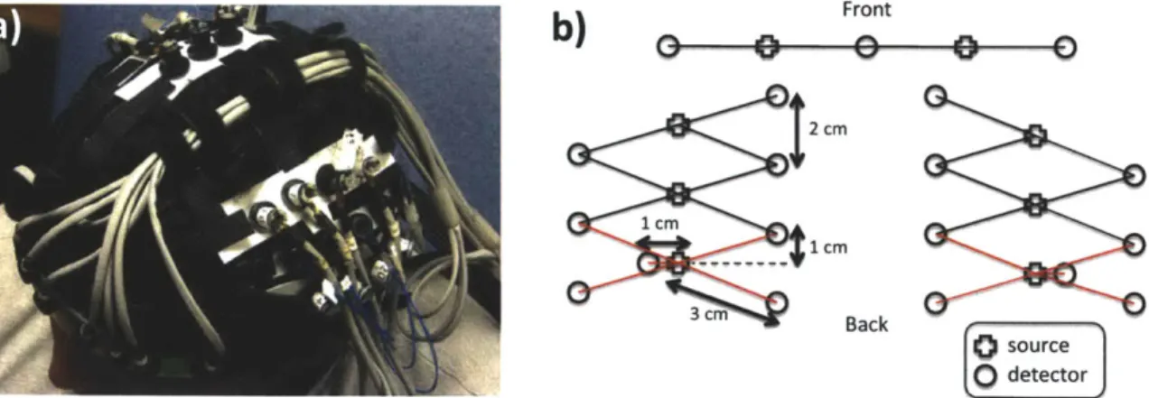
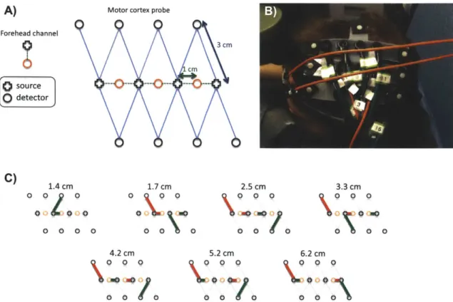
For this study, 6 healthy adult subjects were recruited. The Massachusetts General Hospital Institutional Review Board approved the study and all subjects gave written informed consent. Subjects were instructed to rest while simultaneous BOLD-fMRI and NIRS data were collected. Three 6-minute long runs were collected for each subject. Only the NIRS data was used in this study. The localization and the geometry of the NIRS probe used are shown in Fig. 3-1 a) and b) respectively. Only the two 1 cm SD separation channels and the 8 closest neighbor (3 cm SD separation) channels were used in the analysis.

a)

b)

Front

2

cm

1 cm 1 CM 3 cm Back source 0detector

Figure 2-1: a) Position of the probe over the head of the subjects b) Geometry of the optical probe. Two different SD separations were used: 1 cm and 3 cm. The NIRS channels used for the analysis are shown in red.

Changes in optical density for each SD pair were converted to changes in hemoglobin concentrations using the Beer-Lambert relationship [4, 6, 2] and the SD distances illustrated in Fig. 3-1 b). A pathlength correction factor of 6 and a partial volume correction factor of 50 were used for all SD pairs [26, 27].

2.1.2

Synthetic hemodynamic response

To compare the performance of our two algorithms with existing algorithms, a syn-thetic hemodynamic response was generated using a modified version of a three com-partment biomechanical model [25, 23, 22]. Each parameter of the model was set to the middle of its physiological range [25] which results in an HbO increase of 15

pM and an HbR decrease of 7 pM. The amplitude of this synthetic response was

of the same order as real motor responses on humans using NIRS and those spe-cific pathlength and partial volume correction factors [27]. These synthetic HbO and HbR responses were then added to the unfiltered concentration data with an inter-stimulus interval taken randomly from a uniform distribution (10-35 s) for each individual trial. Over the six-minute data series, we added either 10, 30 or 60 individ-ual evoked responses. The resulting HbO and HbR time courses were then highpass filtered at 0.01 Hz to remove any drifts and lowpass filtered at 1.25 Hz to remove the instrument noise. The filter used was a 3rd order Butterworth-type filter.

Four different methods were then used to recover the simulated hemodynamic re-sponse added to our baseline data. The first two were taken directly from literature and consisted of the standard General Linear Model (GLM) without using a small SD separation measurement and the adaptive filtering (AF) method developed by Zhang et al [52]. The third one was a simultaneous static deconvolution and regression and will be called the static estimator (SE) here for simplicity. The last one was a dynamic Kalman filter estimator (KF).

2.1.3

Signal modeling

For all the methods used in this study, the discrete-time hemodynamic response h at sample time n was reconstructed with a set of temporal basis functions

Nw

h [n] =Z wibi [n] (2.1)

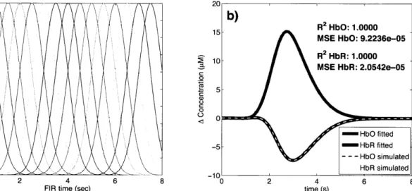
where bi [n] are normalized Gaussian functions with a standard deviation of 0.5 s and their means separated by 0.5 s over the regression time as shown in Fig. 2-2 a). N, is the number of Gaussian functions used to model the hemodynamic response and was set to 15 in our work. Using this set, the noise-free simulated HbO response was fit with a Pearson R2 _{of 1.00 and a mean square error (MSE) of 9.2 x}

10-5 and the noise-free simulated HbR response was fit with an R2 _{of 1.00 and an MSE of}

2.1 x 10-5. The MSE was lower for HbR only because the amplitude of the simulated HbR response was lower. These fits are shown in Fig. 2-2 b). The weights for the temporal bases wi were estimated using the four different methods described in the following sections.

1 20

0 6)

0.9

)V

_b) 2

HbO: 1.0000

0 .515 0.8 MSE HbO: 9.2236e-05

0 2 MSE HbR: 2.0542e-05 0.6 0.5-5 0.4 26 0.3-0.2 0.1- /- b iuae 020 0S 6 80 1 R2 HbR 1.000

FIR time (sec) time (s)

Figure 2-2: a) Temporal basis set used in the analysis. The finite impulse response (FIR) of the temporal basis functions ranged from 0 to 8 s after the onset of the simulated response. b) Noise-free simulated responses (dotted lines) overlapped with the responses recovered with a least-square fit (continuous lines) using the temporal basis set. The RM2 _{and the MSE of the fit are indicated for both and HbR.HbO}

For the standard block average estimator, we modeled the concentration signal in the

3 cm separation channel Y3 [n] by

00

Y3[

Z

h-[k] u[- - k]. (2.2)

k--oo

F [n] is called the onset vector and is a binary vector taking the value 1 when s corresponds to a time where the stimulation starts and 0 otherwise.

For our static simultaneous estimator and our dynamic Kalman filter simultaneous estimator, we modeled the signal in the 3 cm separation channel y3 [n] by a linear

combination of the 1 cm separation signal yi [n] and the hemodynamic response h [n]

by

00 Na

ya [n] = :h [k]u[n -k]+) aiyi[n +1 -i]. (2.3)

k=-oo i=1

Na is the number of time points taken from the 1 cm separation channel to model the superficial signal in the 3 cm separation channel. This value was set to 1 in our work for all three estimators using short SD separation measurements but could be any integer in principle. The ai's are the weights used to model the superficial signal in the 3 cm separation channel from the linear combination of the 1 cm separation signal. The states to be estimated by the static and the Kalman filter estimators were the weights for the superficial contribution ai and the weights for the temporal bases wi. All those weights were assumed stationary in the case of the static estimator, and time-varying in the case of the Kalman filter estimator.

The motivation for Eq. 3.2 is that the residual between the 3 cm channel and the

1 cm channel corresponds to the hemodynamic response of the brain. This is well

justified when the brain activation is detected only in the 3 cm separation channel and when the systemic physiology pollutes both the 1 cm and the 3 cm separation channels. It is a reasonable assumption for cognitive NIRS measurements performed on an adult head. In this case, the hemodynamic response is expected to occur only in the brain tissue and the 1 cm separation channel does not reach the cerebral cortex, making the 1 cm measurement sensitive to scalp and skull fluctuations only. This would also be justified for cognitive measurements on babies by reducing the separation of the 1 cm signal to ensure that this channel remains insensitive to brain hemodynamics. However, our assumption would be violated for specific stimuli (e.g. the Valsalva maneuver) for which the hemodynamic response occurs more globally across the head. Other scenarios that could be troublesome would be if the systemic physiology occurs only in the brain tissue (e.g. an activation-like oscillation a few seconds after the true stimulus response) or if the interference is phase-locked with

the stimulus. In this case, the systemic physiology could potentially be modeled by our temporal basis set (overfitting).

2.1.4

Standard General Linear Model

For this first method, and only for this one, the 1 cm SD separation channels were not used. The pre-filtered concentrations from the 3 cm SD separation were further lowpass filtered at 0.5 Hz using a 3rd order Butterworth filter. Re-expressing Eq. 2.2

in matrix form, we get

Y3 = Uw (2.4)

where y3 is simply the length Nt time course vector y3 [n]

y3

=

[

Y3

[1]

-T

- Y 3 [Nt] _. (2.5)

The columns of U are the linear convolution of the onset vector u [n] with each temporal basis function bi [n]

U =

u

*

b

1

[n]

-.. u * bN [n] (2.6)

and w is the vector containing the weights for the temporal basis wi

-[T

w = W1 ... _{wN, I} (2-7)

The estimates of the weights ' are found by inverting Eq.

Penrose pseudoinverse

n _{= (UTU)l UTy}

3

2.4 using the

Moore-(2.8)

and the hemodynamic response is finally reconstructed with the estimates of the temporal basis weights Ci obtained from *.

the adaptive filter or the Kalman filter), we included a 3rd order polynomial drift as a

regressor. This procedure is used regularly in fMRI analysis. In this case, the matrix

U is expanded

G= [U D (2.9)

where D is an Nt by 4 drift matrix given in the 2.5. The estimates of the weights n' are found by inverting

* = (G T G)- GT Y3. (2.10)

2.1.5

Adaptive filtering

The adaptive filtering technique was taken directly from [52]. Only the salient points are outlined here. The HbO and the HbR responses were recovered independently and the adaptive filter was used for both. The two pre-filtered concentration signals at 1 cm (yi) and 3 cm (y3) were first normalized with respect to their respective standard deviation. This was to ensure that the standard deviation of the two signals used in the computation were close 1 to accelerate the convergence of the algorithm

[52]. The output of the filter, e [In], is then given by

Na

e [n] = y3 [n] )- wk,n yi [n - k] (2.11)

k=0

where the coefficient of the filter, Wk,n, is updated via the Widrow-Hoff least mean

square algorithm [17]:

Wk,n = Wk,n-1 + 2Ae [In - 1]1 Y[In - k]. (2.12)

In our study, w was initialized at Wk,1 = [1 0 0 ... ]T and p was set to 1x10- 4 as in [52].

After trying different values for Na, we identified Na = 1 as the value minimizing the MSE between our simulated and recovered hemodynamic responses. The output e [in]

original scale. The output of the filter was then further lowpass filtered at 0.5 Hz and the hemodynamic response was finally estimated using the standard GLM method (with no drift) by substituting Y3 by e in Eq. 2.8

W = (UTU) UTe (2.13)

where e is simply the length Nt time course vector e [n]

e

=

[e

[1] ... e [Nt]

]

(2.14) and again the hemodynamic response is finally reconstructed with the estimates of the temporal basis weights i obtained from w.

2.1.6

Static estimator

Our static estimator is an improved version of the linear minimum mean square estimator (LMMSE) developed by Saager et al [41, 42]. In their work, they used the small separation signal and an LMMSE to estimate the contribution of the superficial signal in the large separation signal. This superficial contamination was then removed from the large separation signal and the hemodynamic response was then estimated from the residual (large separation signal without the superficial contamination). In our study, we simultaneously removed the contribution of the superficial signal in the

3 cm separation signal and estimated the hemodynamic response.

Eqs. 3.2 and 3.1 can be re-expressed in matrix form

Y3 = Ax (2.15)

2.5, x is the concatenation of the wi's and ai's

X = wi ... wN a, ... aN a (2.16)

and A is the concatenation of the Nt by N, matrix U given by Eq. 3.6 and the Nt

by Na matrix Y

A=

[U

Y

(2.17)

where

Y1 [1] 0 .. .

Syji

[2]

y1

[1]

0

(2.18)

The first Nw columns of A are the linear convolution of the onset vector u

[n]

with each temporal basis function bi

[n]

and the last Na columns of A are simply the signal from the 1 cm separation channel yi [n] delayed by one more sample in each column. In order to compare the different estimators on the same footing, Na was set to 1 for all three estimators using short SD separations. A more explicit expression for A is given in 2.5. The estimates of the weights i are found by inverting Eq. 2.15 using the Moore-Penrose pseudoinverse

k = (ATA) lATy₃ (2.19)

and the hemodynamic response is finally reconstructed with the estimates of the temporal basis weights Cvi obtained from i. This reconstructed response was further lowpass filtered at 0.5 Hz.

2.1.7

Kalman filter estimator

For our dynamic Kalman filter estimator, Eqs. 3.2 and 3.1 need to be re-express in state-space form:

y3 [n] = C [n] x [n] + v [n]

where w [n] and v [n] are the process and the measurement noise respectively. x [n] is the sample n of x given by Eq. 3.5, I is an N, + Na by N, + Na identity matrix and C [n] is an N, + Na by 1 vector whose entries correspond to the nth row of A in

Eq. 2.17. The estimate i [n] at each sample n is then computed using the Kalman

filter [31] followed by the Rauch-Tung-Striebel smoother [40]. The Kalman filter recursions require initialization of the state vector estimate i [0] and estimated state covariance P

[0].

In our study, the initial state vector estimate x [0] was set to the values obtained using our static estimator and the initial state covariance estimate P

[0]

was set to an identity matrix with diagonal entries of 1x10' for the temporal basis states and 5x10-4 for the superficial contribution state. The Kalman filter algorithm was run a first time to estimate the initial state covariance and then run a second time. The initial covariance estimate for the second run was set to the final covariance estimate of the first run. Running the filter twice makes the method less sensitive to the initial guess P [0]. Statistical covariance priors must also be specified for the state process noise cov (w) =

Q

and the measurement noise cov (v) = R. The process noise determines how big the states are allowed to vary at each time step. If this value is small, the estimator will approach the static estimator. If it is large, the state will be allowed to vary significantly over time. In this work, the process noise covariance only contained nonzero terms on the diagonal elements. Those diagonal terms were set to 2.5x10-6 for the temporal basis state and 5x10-6 for the superficial contribution states. This imbalance in state update noise was also used by Diamond et al [7] and caused the functional response model to evolve more slowly than the superficial contribution model. Practically, the measurement noise determine how well we trust the measurements during the recovery procedure. In our study, the measurement noise covariance was set to an identity matrix scaled by 5x102 Different values have been tried for the process noise and the measurement noise covariances. Changing the value of

Q

and R over two orders of magnitude did not result in notable performance changes and we could have drawn all the same (2.21)

conclusions presented in this paper using these alternative

Q

and R values. The values for

Q

and R presented above were empirically determined to minimize the

MSE between the recovered and the simulated hemodynamic response. The algorithm

was then processed with the following prediction-correction recursion [12].

Since the state update matrix is the identity matrix in Eq. 3.3, the state vector x and state covariance P are predicted with

[nn - 1] =i [n - in - 1] (2.22)

P [nmn - 1] = P [n - 1|n - 1] + Q. (2.23)

The Kalman gain K is then computed

K [n] = P [nIn - 1] C [n]T (C [n] P [nIn - 1] C [n]T + R) (2.24)

and the state vector x and state covariance P predictions are corrected with the most recent measurements y3 [n]

i[nn] =:i [nn - 1] + K, (y3 [n] - C [n] i [nIn - 1]) (2.25)

P [nln] = (I - K [n] C [n]) P [nn - 1]. (2.26)

After the Kalman algorithm was applied twice, the Rauch-Tung-Striebel smoother was applied in the backward direction. With the identity matrix as the state-update matrix in Eq. 3.3, the algorithm is given by [18]:

5- [n|Nt] = r [nln] + N [nln]

N

[n + 1|n]- (i, [n + 1|N,] -:k [n + 1|n]) . (2.27)

The complete time course of the estimated hemodynamic response h [n] was then reconstructed for each sample time n using the final state estimates :ki[n|Nt] and the

temporal basis set contained in C [n]

h [n] = C [n]:x [nlNt] . (2.28)

This reconstructed hemodynamic response time course h [n] was further lowpass fil-tered at 0.5 Hz and the standard GLM estimator (with no polynomial drift) was then applied

(UTU) UTi (2.29)

where U is the matrix defined in Eq. 3.6 and

h = [N [1] ... h [N,] (2.30)

to obtain the final weights tiv used to reconstructed the final estimate of the hemo-dynamic response. We observed that these last filtering and averaging steps further improved the estimate of the hemodynamic response compared to reconstructing the hemodynamic response from the final state estimates of the smoother.

2.1.8

Statistical analysis

Only specific channels based on the following criteria were kept in the analysis. The raw hemoglobin concentrations were bandpass filtered with a 3rd order

Butterworth-type filter between 0.01 Hz and 1.25 Hz

[53].

The Pearson correlation coefficient R2 between each 1 cm HbO channel and its 4 closest neighbor 3 cm HbO channels (before adding the synthetic hemodynamic response) were then computed and the

SD pairs for which R2 _{< 0.1 were discarded for the analysis. The mean R2 across}

the selected channels was 0.47 for HbO and 0.22 for HbR. We also computed the Pearson correlation coefficient after adding the synthetic hemodynamic response and similar results were obtained. The mean differences between the R2_{'s computed}

be-fore and after adding the synthetic response was 0.01 for HbO and 0.003 for HbR, with the highest value obtained before adding the synthetic response to the real data.

Those small differences emphasize the fact that the signals were dominated by sys-temic physiology in our simulations. This result also suggests that no resting state measurement is required to select the channels which would benefit from the small separation measurement since the correlation can be estimated from the time course containing brain activation. Zhang et al [51] showed that the adaptive filter method was working well when the correlation between the short and the long separation channel for HbO was greater than 0.6. We used 0.1 in this work to include more channels in the analysis and to show that our state-space method was working well when the initial correlation was lower than 0.5. Using this criterion, 94 out of the 144 possible channels (6 subjects x 3 runs x 8 channels) were kept for further anal-ysis. This represented 65 % of the original data set. The numbers of channels kept for each of the subjects were 16, 14, 13, 17, 19 and 15 respectively. The signal to noise ratio (SNR) for each channel was computed as the amplitude of the simulated hemodynamic response divided by the standard deviation of the time course of the signal. The mean SNR across the selected channels was 0.45 for HbO and 0.38 for HbR.

We used two different metrics to compare the performance of the different algorithms. The first one was the Pearson correlation coefficient R2 between the true synthetic hemodynamic response and the recovered response given by each algorithm. This metric was used to access the level of oscillation in the recovered hemodynamic re-sponse created by the global interference not removed by the algorithms and still contaminating the signal. Since the R2 _{coefficient is scale invariant, it could not give}

any information about the accuracy of the amplitude of the recovered hemodynamic response. To overcome this problem, we also used the mean square error (MSE) as a metric to compare the performance of the different algorithms.

Since the random position of the trials across the same time course can greatly affect the accuracy of the recovered hemodynamic response, we repeated the procedure 30 times with 30 different random onset time instances for each of the 94 selected chan-nels. The mean and the standard deviation of the 2820 R2 _{coefficients (94 channels}

x 30 instances) for each algorithm were then computed after applying the Fisher transformation

z = tanh- 1 (R2_{) (2.31)}

and the results were then inverse transformed. The mean and the standard deviation of the 2820 MSEs were also computed. This procedure was repeated independently for 10, 30 and 60 trials in each six-minute data series. The different algorithms were compared together by computing two-tailed paired t-tests on their MSEs and Fisher transformed R2 _{coefficients.}

2.2

Results

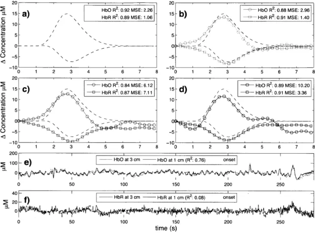
Typical time courses of the recovered hemodynamic response overlapped with the true simulated response are shown in Fig. 2-3 a) to d) for the four algorithms tested. The SNR for this particular simulation was 0.33 for HbO and 0.81 for HbR. The R2_'s

and the MSEs for HbO and HbR are shown in the legend of each individual panel. Those individual results were obtained from a single simulation with 10 trials. The time courses for this specific simulation are shown in panel e) for HbO and f) for HbR. Both the initial 1 cm channel and the 3 cm channel containing the added synthetic hemodynamic responses are shown as well as the position of the 10 individual onset times. The R2 between the initial 1 cm channel and the initial 3 cm channel (no response added) is also shown in the legend of panel e) and f) for HbO and HbR respectively. All concentrations are expressed in micromolar (tM) units.

The summary R2 _{statistics over all subjects, all channels and all instances are shown}

in a bar graph in Fig. 2-4 for both HbO and HbR. These values represent the Pearson R2 coefficients computed between the recovered and the simulated hemodynamic

responses. The bars represent the mean and the error bars represent the standard

deviation. Both the mean and the standard deviation were computed on the Fisher transformed values and then inverse transformed. Two-tailed paired t-tests on the

20 20

2HbO R 2 0.92 MSE: 2.26 HbO R 2:0.88 MSE. 2.96

1 15 - ) HbOR2: 9 MSE:- 1 ) HbRR2 091 MSE140

C HbR R2: 0.89 MS E: 1.06 10- -4 10- / N A/ 5 -5 -5 -10 1 0 1 2 3 4 5 6 7 8 0 2 4 5 6 7 20 2 e.1

-C HbO R 2 :0.84 MSE: 6.12 e HOR2:.9ME 0

-15 -C)15-d2 E3 HbR R2: 0.87 MS E: 7.11E3 HRR 09 I 10 - -Cz 5 --0 ' C 0 010 o5 -0

5--5--10

)HbO

at 3 cm - HbO at 1 cm (R 2: 0.76) onset 100-1) 0 0 50 100 150 200 250 4011 0- f)HbR at 3 cm - HbR at 1 cm (R2: 0.08) onset 0 20 0 50 100 150 200 250 time (s)

Figure 2-3: a) to d) Typical time courses of the recovered hemodynamic responses overlapped with the simulated hemodynamic response. For these specific traces, the SNR was 0.33 for HbO and 0.81 for HbR. R2 _{coefficients and MSEs between the}

recovered (circles) and the simulated (dashed) response are shown in the legends. a) Kalman filter estimator b) Static estimator c) Adaptive filter d) Standard GLM with 3V order drift. e) HbO and f) HbR time courses of the 3 cm channel (with synthetic responses added) overlapped with the 1 cm channel. The positions of the onset time are also shown and the correlation coefficients between the 1 cm and the

3 cm channels (before adding synthetic responses) are indicated in parenthesis.

Fisher transformed values were performed between all the different estimators and statistical significance at the level p < 0.05 is illustrated by a black line over the bars

for which a significant difference was observed. In our three simulations using 10,

30 and 60 trials respectively, the R2's for HbO and HbR obtained using our Kalman filter dynamic estimator were significantly higher (p < 0.05) than the ones obtained

using the adaptive filter. Moreover, the R2's obtained were higher with the Kalman filter than with the static estimator. These differences were significant (p < 0.05)

except in our 10 trial simulation for HbO.

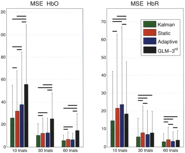
Similarly, the summary MSE statistics over all subjects, all channels and all instances are shown in Fig. 2-5. These values represent the mean square error computed be-tween the recovered and the simulated hemodynamic responses. The bars represent the mean while the error bars represent the standard deviation. Two-tailed paired t-tests were performed between all the different estimators and statistical significance at the level p < 0.05 is illustrated by a black line over the bars for which a significant

difference was observed. The MSEs obtained for HbO and HbR in our three simu-lations (10, 30 and 60 trials) were significantly lower (p < 0.05) with our Kalman

filter estimator than with the adaptive filter. Futhermore, the MSEs obtained with the Kalman filter were also lower (p < 0.05) than the ones obtained with the static

estimator for both HbO and HbR in our three simulations.

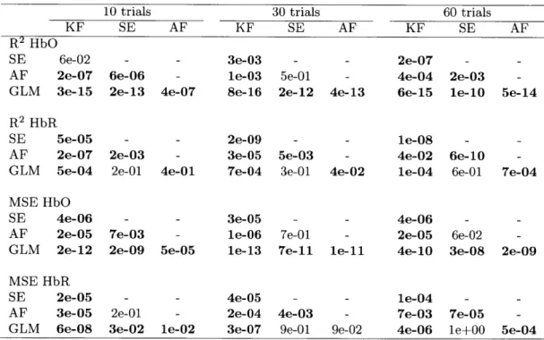
Table 2.1 summarizes the statistical analysis over all the subjects, all the channels and all the instances for both HbO and HbR and for the simulations with 10, 30 and

60 trials. Each algorithm was compared to every other. The values shown are the

p-values obtained from a two-tailed paired t-test. Statistical differences at the level

p < 0.05 are indicated with bold script. These p-values were computed from the data

R2 HbO

-a

1

.Ilk

.I

10 trials 30 trials 60 trials

R

2

_HbR

0.81 0.6 0.41 0.2 0

Kalman

Static

-

Adaptive

-

GLM-3rd

10 trials 30 trials 60 trials

Figure 2-4: Pearson R2 _{coefficients between simulated and recovered hemodynamic}

responses. The bars represent the means and the error bars represent standard devia-tions computed accross all subjects, all channels and all intances. The means and the standard deviation were computed in the Fisher space and then inverse transformed. Two-tailed paired t-tests were performed on the Fisher transformed R2_{'s. Statistical} differences (p < 0.05) between the four algorithms are indicated by black horizontal

lines over the corresponding bars.

1

0.8

0.6

0.4

MSE

HbO

120

10 trials 30 trials 60 trials

Figure 2-5: Mean squared errors (MSE) between simulated and recovered hemody-namic responses. The bars represent the means and the error bars represent the standard deviations computed accross all subjects, all channels and all instances. Two-tailed paired t-tests were performed between the four estimators and statisti-cal differences at the level p < 0.05 are indicated by black horizontal lines over the

corresponding bars.

60 trials

Table 2.1: Cross-comparison of the different algorithms. P-values for the two-tailed paired t-tests accross all subjects, all channels and all intances are shown. For the R2 coefficients, the tests were performed on the Fisher transformed values. Bold face indicates significant difference at the p < 0.05 level. KF: Kalman filter estimator, SE: Static estimator, AF: Adaptive filter, GLM: Standard GLM with ₃rd order drift.

10 trials 30 trials 60 trials

KF SE AF KF SE AF KF SE AF

R2 _HbO

SE 6e-02 - - 3e-03 - - 2e-07 -

-AF 2e-07 6e-06 - le-03 5e-01 - 4e-04 2e-03

-GLM 3e-15 2e-13 4e-07 8e-16 2e-12 4e-13 6e-15 le-10 5e-14

R2 HbR

SE 5e-05 - - 2e-09 - - le-08

-AF 2e-07 2e-03 - 3e-05 5e-03 - 4e-02 6e-10

-GLM 5e-04 2e-01 4e-01 7e-04 3e-01 4e-02 le-04 6e-01 7e-04

MSE HbO

SE 4e-06 - - 3e-05 - - 4e-06 -

-AF 2e-05 7e-03 - le-06 7e-01 - 2e-05 6e-02

-GLM 2e-12 2e-09 5e-05 le-13 7e-11 le-11 4e-10 3e-08 2e-09

MSE HbR

SE 2e-05 - - 4e-05 - - le-04 -

-AF 3e-05 2e-01 - 2e-04 4e-03 - 7e-03 7e-05

2.3

Discussion

2.3.1

Simultaneous filtering and estimation

One of the salient features of our Kalman filter estimator is that it filters the global interference and simultaneously estimates the hemodynamic response. This feature resulted in a more accurate recovery of the hemodynamic response with our Kalman filter estimator compared to the adaptive filter, for which the filtering and the es-timation were performed in two distinct steps. Independent regression of the small separation channel potentially removes contributions of the hemodynamic response in the signal which lead to an underestimation of the hemodynamic response thereafter. Our Kalman filter estimator avoids this pitfall. Compared to the adaptive filter, our Kalman filter estimator showed significant improvements at the p < 0.05 level in both HbO and HbR recoveries for our 10, 30 and 60 trial simulations. Those improvements

were observed in both Pearson R2 and MSE metrics.

2.3.2

Dynamic versus static estimation

The systemic interference present in NIRS data is non-stationary. This has been nicely shown by Lina et al [33] who performed a detailed wavelet analysis of resting NIRS data with blood pressure, respiratory and heart rate data acquired simultaneously on awake human subjects. The amplitude of the systemic physiology measured by the 1 cm and the 3 cm channel depends on the respective pathlength of the light for each channel. Systemic physiology could alter the optical properties of the tissue over time. As a result, a sustained change in absorption could modify the pathlength of the light independently in the 1 cm and the 3 cm channel, modifying at the same time the relative amplitude of the systemic physiology detected in each channel. This feature of the systemic interference explains why our Kalman filter, which is a dynamic estimator, performed better than the static estimator. Using our Kalman

filter estimator, improvements in the HbO and HbR recovery were observed in both the Pearson R2 and the MSE metrics compared to the static estimator. All these improvements were significant at the p < 0.05 level except for the HbO Pearson R2

improvement which was not significant in our 10 trial simulation.

2.3.3

HbO versus HbR

In their wavelet analysis, Lina et al [33] also showed that the HbO time courses were more contaminated by global interference than the HbR time courses. As such, the correlation between the 1 cm and 3 cm channel should be higher for HbO than HbR, and filtering methods using 1 cm SD separations should work better for HbO than for HbR. In our data, the mean initial Pearson R2 _{correlation between the 1}

cm and 3 cm signals were higher for HbO than HbR (0.47 vs 0.22). Comparing our Kalman filter estimator with the standard block average estimator, the p-values obtained in the t-tests performed on the Fisher transformed Pearson R2_{'s and the}

MSEs were at least five orders of magnitude lower for HbO than HbR. This indicates that the improvements observed with our Kalman filter were more prominent for HbO than HbR. This better performance in the recovery of HbO over HbR using a small separation method was also reported by Zhang et al [51] using their adaptive filter.

2.3.4

Impact of initial correlation

In the case where the systemic physiology present in the 3 cm separation did not correlate with the systemic physiology present in the 1 cm channel, the performance of the Kalman filter was similar to the standard GLM. In this case, the model cannot reproduce the data and the ai coefficients in Eq. 3.2 converge to zero. As such, the wi's estimated by the Kalman filter are very close to the ones obtained using the GLM. An important point is that in the case of low initial R2 _{coefficients (0.1 <}

decrease the performance of the recovery compared to the GLM. On the other hand, the performance of the adaptive filter for (0.1 < initial R2 < 0.2) was worst than the GLM. This counter-performance of the adaptive filter for poor initial correlation between the short and the long channel was also reported by Zhang et al [51]. These findings suggest that the Kalman filter can be used even if the correlation between the 1 cm and the 3 cm channel is low as opposed to the adaptive filter. In the worst case, the Kalman filter will be as good as the standard GLM. However, the higher the initial correlation between the 1 cm and the 3 cm channel is, the more significant is the improvement using a small separation measurement. This is illustrated by the larger improvement obtained for HbO than HbR when using a small separation measurement together with our Kalman filter.

2.3.5

Technical notes

The MSEs obtained in our simulations and presented in Fig. 2-5 were lower for HbR than HbO. This occurred because the amplitude of the simulated HbR response was lower than the simulated HbO response which resulted in lower MSEs for HbR. This is illustrated for noise-free data in Fig. 2-2b.

For all the results presented in this paper, a single time point was taken from the 1 cm channel to regress the 3 cm channel. In practice, this value could be any integer.

A simple phase shift (delay) between the 3 cm and 1 cm channel would be taken into

account by using multiple time points from the 1 cm. In this case, all the a's in Eq.

3.2 would converge to zero except for one a at the value of i corresponding to the

shift between the two signals in terms of number of sample points. Different values for Na were tested during our simulations. With the adaptive filter, we obtained better results using a single point than using 100 points as in Zhang et al [52]. Using

100 points results in overfitting the signal which removes more of the hemodynamic

response contribution than using a single point. This is another pitfall of the non-simultaneous recovery and filtering feature of the adaptive filter which is avoided with

our Kalman filter. Finally, we did not observe any improvement when using multiple points with our Kalman filter, suggesting that no delays were present in our data between the 1 cm and the 3 cm channel.

The Gaussian temporal basis functions used in this work allow us to model different hemodynamic responses with different shapes and components. This includes a po-tential initial dip and post-stimulus undershoot, responses with a double bump and negative responses. It is also easy to use additional Gaussian functions to extend this method for longer stimuli, making the temporal basis set used in the present work very general and less restrictive. However, as stated in section 2.1.3, the drawback for using a more general set is the potential overfitting of phase-locked systemic phys-iology. This could be avoided using a more restrictive temporal basis set such as a gamma-variant function and its derivatives [24, 1, 21, 14], and at the same time could potentially reduce the number of parameters to estimate.

We tested different values for the separation between the basis and also different values for the width of the Gaussians. The values of 0.5 second for both the separation and the width presented in this paper resulted in the lowest MSEs between the recovered and the simulated responses and highest R2_{'s. The separation between our temporal}

basis Gaussians and their widths was three times lower than the values used by Diamond et al

[7].

In order to compare the four methods used in this work on the same footing, we used temporal basis functions for each estimator. For the standard GLM estimator, the adaptive filter and the Kalman filter, we have also tried to replace the final step of using the GLM with a temporal basis set by a simple block average without using any temporal prior. For all these three estimators, using temporal basis functions in the final step further improved the recovery of both HbO and HbR. The MSEs between the recovered and the simulated hemodynamic response were lower when temporal basis were used than when a simple block average without temporal basis was applied. Similarly, the R2's computed between the recovered and the simulated

responses were higher when temporal basis were used in the final block average step. This result raises the importance of using temporal priors to reduce the dimensionality of the estimation problem.

As stated in section 2.1.7, changing the state process noise and the measurement noise priors over two orders of magnitude did not affect the performance of our Kalman esti-mator. For HbO, no differences could be observed (two-tailed paired t-test, p < 0.05)

between the MSEs recovered using values for the process noise or the measurement noise ten times lower or higher than the ones presented in section 2.1.7. For HbR, small differences in the MSEs were observed but these results did not change any conclusions drawn in this paper. The MSEs recovered with our Kalman filter in this case were still the lowest of the four estimators.

2.3.6

Future directions

As mentioned in Zhang et al [51], an important question is whether an additional short separation optode is required for each longer separation optode or whether a single one is sufficient. Although the systemic interference is thought to be global in the brain, it might be reflected differently in the NIRS data collected over different regions of the head. Sources of variation include blood vessel size which might affect the amplitude of the recovered response but also blood vessel length and geometry which might give rise to phase mismatches between different NIRS channels. Studies using multiple small SD separation optodes at different locations over the head should be performed in the future to address this question.

2.4

Summary

In summary, we filtered the global interference present in NIRS data by using addi-tional small separation optodes and we simultaneously estimated the hemodynamic

response using a dynamic algorithm. Our dynamic Kalman filter performed bet-ter than the traditional adaptive filbet-ter, the static estimator and the standard block average estimator for both HbO and HbR recovery. These results were consistent with the fact that dynamic estimation better captures the non-stationary behavior of the systemic interferences in NIRS and that the simultaneous filtering and estima-tion prevents underestimaestima-tion of the hemodynamic response. The algorithm is easily implementable and suitable for a wide range of NIRS studies.

2.5

Appendix: Design matrix

The explicit expression for D in Eq. 2.9 is given by 1 1/Nt 12/N 13

/N?

1 2/Nt 22

/Ne

23/Nt

D 1 3/Nt 32_{/Ne 3}3_/Nte

1 Nt/Nt N/N 2 N/N|

The dimension of the matrix D is N, by 4. Each column is normalized by its highest value to keep the matrix G well conditioned and to avoid numerical errors during the inversion in Eq.2.10.

The explicit expression for A in Eq. 2.17 is given by b1 [1] b1 [2] b1 [Nb] 0 0 b1 [1] b1 [2] b1 [Nb] 0 b2 [1] b2 [2] b2 [Nb] 0 0 b2 [1] b2 [2] b2 [Nb] 0 ... bN. [1] ... bN. [2] ... bN. [Nb] 0 0 ... bN. [1] ... bN. [2] ... bN [Nb] 0 y1 1N Y1 [2] yj [Nt]

Nb is the length of each temporal basis function and was 80 in our work due to the

10 Hz temporal resolution and 8 s FIR for our temporal basis functions. The vertical

dimension of matrix A corresponds to Nt, the total number of time points in the entire time course. The number of copies of the temporal basis functions corresponds to the number of trials (or stimuli) in the specific time course (i.e. if the run contained

10 trials, then 10 copies of the temporal basis set will appear in the corresponding A

matrix). 0 Y1 [Nt -0 0 Y1~l 1] ... y1[Nt - Na + 1]

Chapter 3

Impact of the short channel

location

This section was submitted for publication:

Gagnon, L., Cooper, R. J., Yucel, M. A., Perdue, K., Greve, D. N., and Boas, D. A. (2011). "Short separation channel location impacts the performance of short channel regression in NIRS." submitted

The main contribution of this chapter is to quantify the performance of the short separation method as a function of the relative distance between 3 cm NIRS channels containing the brain signal and 1 cm channels used as a regressors. We investigated this relationship with both simulations and real functional data. NIRS measurements including several short separation channels spread across the probe were acquired on

6 human subjects. The simulations were performed by adding a synthetic

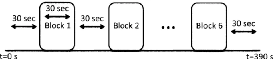
hemo-dynamic response to the resting-state NIRS data. NIRS signals were also collected during a series of finger tapping blocks for each of the 6 subjects. In both cases, the performance of the short separation regression was characterized for different short