HAL Id: hal-00317583
https://hal.archives-ouvertes.fr/hal-00317583
Submitted on 7 Sep 2004
HAL is a multi-disciplinary open access
archive for the deposit and dissemination of
sci-entific research documents, whether they are
pub-lished or not. The documents may come from
teaching and research institutions in France or
abroad, or from public or private research centers.
L’archive ouverte pluridisciplinaire HAL, est
destinée au dépôt et à la diffusion de documents
scientifiques de niveau recherche, publiés ou non,
émanant des établissements d’enseignement et de
recherche français ou étrangers, des laboratoires
publics ou privés.
SuperDARN data
C. L. Waters, B. J. Anderson, R. A. Greenwald, R. J. Barnes, J. M.
Ruohoniemi
To cite this version:
C. L. Waters, B. J. Anderson, R. A. Greenwald, R. J. Barnes, J. M. Ruohoniemi. High-latitude
poynt-ing flux from combined Iridium and SuperDARN data. Annales Geophysicae, European Geosciences
Union, 2004, 22 (8), pp.2861-2875. �hal-00317583�
SRef-ID: 1432-0576/ag/2004-22-2861 © European Geosciences Union 2004
Annales
Geophysicae
High-latitude poynting flux from combined Iridium and
SuperDARN data
C. L. Waters1, B. J. Anderson2, R. A. Greenwald2, R. J. Barnes2, and J. M. Ruohoniemi2
1School of Mathematical and Physical Sciences, The University of Newcastle University Drive, Callaghan, 2308 NSW, Australia
2The Johns Hopkins University Applied Physics Laboratory 11100 Johns Hopkins Road Laurel, MD 20723-6099, USA Received: 17 February 2003 – Revised: 1 May 2004 – Accepted: 25 May 2004 – Published: 7 September 2004
Abstract. Field-aligned currents convey stress between the
magnetosphere and ionosphere, and the associated low al-titude magnetic and electric fields reflect the flow of elec-tromagnetic energy to the polar ionosphere. We introduce a new technique to measure the global distribution of high latitude Poynting flux, S||, by combining electric field
esti-mates from the Super Dual Auroral Radar Network (Super-DARN) with magnetic perturbations derived using magne-tometer data from the Iridium satellite constellation. Spher-ical harmonic methods are used to merge the data sets and calculate S||for any magnetic local time (MLT) from the pole
to 60◦magnetic latitude (MLAT). The effective spatial res-olutions are 2◦MLAT, 2 h MLT, and the time resolution is about one hour due to the telemetry rate of the Iridium mag-netometer data. The technique allows for the assessment of high-latitude net S|| and its spatial distribution on one hour
time scales with two key advantages: (1) it yields the net S||
including the contribution of neutral winds; and (2) the re-sults are obtained without recourse to estimates of ionosphere conductivity. We present two examples, 23 November 1999, 14:00–15:00 UT, and 11 March 2000, 16:00–17:00 UT, to test the accuracy of the technique and to illustrate the dis-tributions of S|| that it gives. Comparisons with in-situ S||
estimates from DMSP satellites show agreement to a few mW/m2 and in the locations of S|| enhancements to within
the technique’s resolution. The total electromagnetic energy flux was 50 GW for these events. At auroral latitudes, S||
tends to maximize in the morning and afternoon in regions less than 5◦in MLAT by two hours in MLT having S
||=10
to 20 mW/m2and total power up to 10 GW. The power pole-ward of the Region 1 currents is about one-third of the total power, indicating significant energy flux over the polar cap.
Key words. Magnetospheric physics (current systems:
magnetosphere-ionosphere interactions) – Ionosphere (in-struments and techniques)
Correspondence to: C. L. Waters (colin.waters@newcastle.edu.au)
1 Introduction
The interaction of the solar wind with the Earth’s magnetic environment in space gives rise to an electromagnetic dy-namo connecting the magnetosphere with the ionosphere via electric fields and currents. Quantifying the energy trans-fer between the magnetosphere and ionosphere is fundamen-tal to understanding the dynamics of the high-latitude iono-sphere and thermoiono-sphere. The two major mechanisms of en-ergy transfer at the ionosphere are particle precipitation and energy in the electromagnetic fields or Poynting flux. Parti-cle energy deposition causes ionization and heating through collisions in the ionosphere and may be remote sensed us-ing auroral ultra-violet (UV) imagus-ing (e.g. Rees et al., 1988; Lummerzheim et al., 1997). Electromagnetic energy incident on the topside ionosphere is either dissipated as Joule heating (e.g. Cole, 1962, 1975) or converted into mechanical energy of neutral winds (Fujii et al., 1999; Thayer, 2000). Particle precipitation and Poynting flux have different spatial distri-butions but the latter appears to account for roughly a factor of 2 more total power (Thayer et al., 1995; Lu et al., 1998; Anderson et al., 1998).
For quasi-steady state fields, the electromagnetic energy is expressed by Poynting’s theorem as
1
µ0
∇ ·(E × b) = −J · E , (1)
where b is the perturbation magnetic field caused by the Birkeland and ionosphere currents, and J ·E is the energy dissipation term that describes the rate of electromagnetic en-ergy transferred to the medium, in this case, the neutral gas. Experimental studies of high latitude electrodynamic energy transport to the ionosphere have used three approaches: (i) incoherent scatter radar (ISR) measurements, (ii) ground-based magnetometer data supplemented with radar data, au-roral images and satellite data and (iii) low Earth orbit (LEO) satellite measurements. The first two methods use the right-hand side of Eq. (1), estimating J and E from the mea-surements (cf. Thayer et al., 1995 for a discussion of this
technique), whereas the third method uses in-situ measure-ments of b. The ISR technique is arguably the most power-ful, since the electric field, electron/ion density, and electron and ion drift velocities may be derived from the ISR data (Vickrey et al., 1982; Thayer, 2000). For an assumed spatial distribution of the Hall and Pedersen conductivities (using a neutral atmosphere model) in concert with the ISR data, one can estimate the partitioning of energy between neutral wind acceleration and Joule heating (e.g. Thayer et al., 1995) over the spatial coverage of the radar. Estimating net electrody-namic energy exchange over the region from 60◦to the pole at all longitudes using existing methods requires various as-sumptions of ionosphere conductivity and neutral wind prop-erties. LEO methods do not necessarily require conductivity and neutral wind assumptions but are limited to long time intervals (∼ months) giving averaged global estimates.
The determination of the right-hand side of Eq. (1) is com-plicated by the significant role that the velocity of the neutral gas can play in energy dissipation (Thayer et al., 1995; Lu et al., 1995). If the neutral gas has a velocity U , the electric field in the neutral gas frame is Eu=E+ U ×B, and the
right-hand side of Eq. (1) can be written as (Thayer and Vickrey, 1992)
J · E = J · Eu+U · (J × B) . (2)
The Joule dissipation is given by Qj=J ·Eu, since
U ·(J ×B) is the mechanical work done on the neutral gas.
The conductivity tensor, 6, in terms of the Pedersen and Hall conductivities, is usually defined in the neutral gas frame so that J =6·Eu(e.g. Fujii et al., 1998). In the absence of
in-formation about neutral winds, it is customary to estimate the Joule heating as Qj*=6PE2 (e.g. Kosch and Nielsen,
1995; Lu et al., 1996). In general, Qj* is neither the
to-tal dissipation, J ·E, nor the Joule heating rate, Qj. Only
for U =0 do we have Qj* = Qj=J ·E. Thayer et al. (1995)
called Qj* the passive thermosphere approximation to the
dissipation rate. Because of the complexities introduced by the neutral wind, determining the total electromagnetic en-ergy dissipation and its division between Joule heating and mechanical work has been a subject of detailed study.
Energy transfer in the high-latitude ionosphere has also been studied using LEO satellite data. Foster et al. (1983) analyzed AE-C satellite measurements of ion drift veloci-ties and particle precipitation in the ionosphere F region for the period 1974–1978. They used an empirical model for the Pedersen conductivity and set the neutral wind velocity to zero. Typical values obtained were 35 GW for Kp 0−3
and 85−100 GW for Kp 3−6. Heelis and Coley (1988)
an-alyzed DE 2 satellite ion drift velocity, temperature and ion concentration data. They assumed a zero neutral wind ve-locity, fixed the ion-neutral collision frequency at 1 s−1and imposed a diffusive equilibrium model for the ion concentra-tion. They proposed that frictional heating is more effective on the dawn side compared to the dusk side high-latitude atmosphere. Estimates of Poynting flux that bypassed the need for imposing neutral wind and ionosphere conductivity models were reported by Kelley et al. (1991). Using fluxgate
magnetometer and ion drift meter data along 2 high-latitude passes of the HILAT spacecraft, Kelley et al. identified small regions of upward Poynting flux. On a more global scale, Gary et al. (1995) examined 576 high-latitude passes of flux-gate magnetometer and ion drift velocity data from the DE 2 spacecraft. They presented global maps of Poynting flux av-eraged over the satellite lifetime. All previous studies of cur-rents linking the ionosphere and magnetosphere using LEO methods achieve global coverage but with poor temporal res-olution, usually of the order of months.
Obtaining realistic estimates of the global Poynting flux is difficult because the magnetospheionosphere system re-configures globally in response to changing solar wind con-ditions. Localized measurements using incoherent scatter radars or single satellite measurements do not provide the global context. Statistical averages provide essential knowl-edge of the general intensity and distribution of energy in-put (Gary et al., 1995; Kosch and Nielsen, 1995; Thayer, 2000) but may not reflect the drivers of ionospheric dynam-ics for particular conditions. One approach is to use arrays of ground stations to provide global coverage with good time resolution. The availability of data from numerous ground stations has facilitated techniques to obtain nearly instan-taneous maps of ionospheric equivalent current (Kamide et al., 1981). An extension of these techniques is the Assimila-tive Mapping of Ionospheric Electrodynamics (AMIE) pro-cedure (Richmond and Kamide, 1988). Using statistical models for the conductivity and convection electric fields, to-gether with various ground and space based data sets, AMIE specifies the ionosphere currents and electric fields (e.g. Lu et al., 1996).
Since electromagnetic energy accounts for most of the en-ergy flow from the magnetosphere to the ionosphere, it is important to obtain independent measures of the global high latitude Poynting flux, free from assumptions of conductiv-ity and neutral wind models. In this paper we introduce a technique to estimate the distribution of Poynting flux at all latitudes poleward of 60 degrees from electric and magnetic field measurements derived directly from distributed radar and satellite observations. This approach complements pre-vious estimates of high-latitude energy flux. It is more global than those derived from incoherent scatter radars and does not require models of ionosphere conductivity or thermo-sphere neutral winds. However, it provides the net energy flux with no information on the partitioning of energy be-tween Joule heating and mechanical work. The technique is more direct compared with methods such as AMIE which rely on ionosphere conductivity models and do not include the influence of neutral winds. However, at present the tech-nique suffers from significantly coarser time resolution. Sec-tion 2 discusses the technique. Results from two intervals are presented in Sect. 3 and the results are discussed and summa-rized in Sect. 4.
2 Poynting flux estimation technique
We use the left-hand side of Eq. (1) to derive global maps of the high-latitude Poynting flux. Integrating Eq. (1) over a closed surface, a, and using the divergence theorem gives
1 µ0 I a (E × b) · da = − Z v E · J dv . (3)
Consider a volume bounded by the surface of the Earth, a par-allel surface at ∼300 km altitude covering latitudes greater than, say 60◦, and connected to the Earth’s surface by a straight radial surface. Poynting flux enters from the mag-netosphere through the top surface and we assume that no energy flows through the bottom or side surfaces (Kelley et al., 1991). The net electromagnetic power dissipated in the volume is equal to the total power flowing through the up-per surface, as described by the left-hand side of Eq. (3). We define the Poynting flux into the topside ionosphere as
S||= −
1
µ0
(E × b) · ˆr , (4)
where ˆr is the unit vector along the geomagnetic field (ap-proximately radial) and S|| is positive downward.
Equa-tion (4) holds provided that E and b are determined in an inertial (non-rotating) frame of reference fixed relative to the Earth. For application to the ionosphere we use the Alti-tude Adjusted Corrected Geomagnetic (AACGM) latiAlti-tude, magnetic local time coordinates (Baker and Wing, 1989) and evaluate E and b at 300 km altitude (cf. Waters et al., 2001). When determining S|| from LEO satellite data one must
re-move the spacecraft velocity, usat, in evaluating plasma drifts or subtract the −usat×B electric field from direct measure-ments of electric fields. For radar determinations of E one must remove the radar velocity from the Doppler velocity de-terminations. Since the ambient electric field is very small, the b measured by satellites is to a very high accuracy the same as that in an inertial frame. Up until now, global scale in-situ measurements of both E and b on time scales of less than hours have not been possible.
2.1 Estimating the electric field
The electric field is derived by detecting ion convective mo-tions in the ionosphere F region. At ∼300 km altitude the geomagnetic field-aligned electric field is negligible and the transverse electric fields drive the plasma with a convection velocity,
v = −E × B/B2. (5)
Measurements of v in Eq. (5) are available from the Super Dual Auroral Radar Network (SuperDARN) which employs over-the-horizon radar technology to probe the high-latitude ionosphere by detecting signal scattered back to the radar by density irregularities. SuperDARN is an international col-laboration of HF radars in the polar regions and the cover-age in the Northern Hemisphere is shown in Fig. 1 of Shep-herd and Ruohoniemi (2000). Technical details of the radars
Figure 1 -10 -5 0 5 10 B X ( n T ) -10 -5 0 5 10 B Y ( n T ) -10 -5 0 5 10 B Z ( n T ) 11 March 2000 -180 -90 0 90 180 C lo c k ( °) 12:00 13:00 14:00 15:00 16:00 17:00 18:00 19:00 20:00 21:00 22:00 UT 10 5 0 B ( n T )
Fig. 1. Interplanetary magnetic field data in GSM coordinates for 11 March 2000 from the ACE spacecraft. Vertical dashed lines show the approximate period of time at ACE that corresponds to the solar wind at Earth during the 16:00–17:00 UT interval ana-lyzed here. Solar wind data are not available after 04:00 UT on this day.
are described in Greenwald et al. (1985). In common mode, the radars scan through 16 successive azimuthal directions or beams spaced by 3.3◦, with an integration time of 7 s per beam (Ruohoniemi and Baker, 1998). The Doppler shifts in the backscattered returns provide estimates of the velocity in Eq. (5). The radars rotate with the Earth and this effect is removed from the line of sight velocities by subtracting the projection of the radar velocity along the line of sight. The resulting velocities and hence electric fields are evaluated in an Earth centered, non-rotating frame.
Velocity estimates of the plasma convection may be ob-tained by vector addition of the line-of-sight measurements within common volumes (Greenwald et al., 1995). A technique that uses all available radar data to map the global convection pattern was described by Ruohoniemi and Baker (1998). After median filtering to improve data in-tegrity, the data are overlaid on a spatial grid with each square cell measuring ∼110 km on a side. The electric field is ex-pressed as the gradient of an electrostatic potential which is expanded in terms of spherical harmonic functions and the coefficients are determined using a least-squares formu-lation. The radar velocity measurements are supplemented with velocity information from the statistical model of Ruo-honiemi and Greenwald (1996), keyed to the IMF conditions. 2.2 Estimating the perturbation magnetic fields
The Iridium satellite constellation consists of over 70 three-axis stabilized satellites in 6 polar orbit, meridian planes. The
onboard magnetometers measure the magnetic field in the Earth centered radial, satellite cross and along track direc-tions. However, only the cross track component data are suit-able (Anderson et al., 2000, 2002). The magnetometer data from the Iridium satellites are available at an average sample period around 200 seconds. Using data from all satellites in each orbit plane compensates for the long sampling interval. The procedure for extracting the cross-track magnetic field perturbation signal from the Iridium satellite data was de-scribed by Anderson et al. (2000). Briefly, the IGRF model magnetic field is subtracted from the Iridium magnetometer data, corrections for cross-talk, sensor orientation and offsets are applied and the resulting cross-track magnetic field data are high pass filtered. The procedure for obtaining the mag-netic field, b, due to Birkeland currents at any location from the cross-track Iridium magnetometer data, using spherical harmonic data fitting techniques, is described in Waters et al. (2001).
2.3 Global Poynting flux
The SuperDARN and Iridium magnetometer data can be combined to give the Poynting flux by application of Eq. (4). With the present Iridium magnetometer data average sam-ple rate, Anderson et al. (2000, 2001) have shown that the Iridium data need to be integrated over about one hour to ob-tain a latitude resolution of roughly 2◦. For the time being, this limits our calculation of global Poynting flux to intervals when solar wind conditions are stable over an hour or longer. This is a dramatic improvement on global energy estimates where the data were averaged over the DE 2 spacecraft life-time (Gary et al., 1995) and is more comparable with the life-time taken for an ∼800 km altitude satellite pass (∼30 min). The SuperDARN data provides global electric field maps on time scales as short as 2 min (Ruohoniemi and Baker, 1998). This much shorter time scale allows verification that the global plasma convection is stable over the accumulation time used for the Iridium data. To calculate the Poynting flux, the 2-min SuperDARN derived electric field values were averaged over the intervals used to accumulate the Iridium data.
3 Event results
We present results for two intervals, Event 1 from 16:00– 17:00 UT on 11 March 2000 and Event 2 from 14:00– 15:00 UT on 23 November 1999. These events were chosen based on the quality of the field-aligned currents obtained from Iridium, the spatial coverage of backscatter returns in SuperDARN data and the stability of the SuperDARN de-rived convection pattern. We first discuss the solar wind/IMF conditions and the prevailing geophysical conditions for each case before considering the Poynting flux results.
3.1 Event 1: 16:00–17:00 UT, 11 March 2000
The interplanetary magnetic field (IMF) data obtained by the Active Composition Explorer (ACE) spacecraft for 11 March
2000 are shown in Fig. 1. Solar wind proton data are not available from ACE but key parameter data from WIND (180 to 175 REsunward of Earth) show that the solar wind speed
varied slowly between 370 and 320 km/s on this day and was near 340 km/s from 12:00 to 18:00 UT. This gives a nominal time lag of 1.1-hours between ACE at the L1-point and Earth. Dashed lines in Fig. 1 indicate the 14:54–15:54 UT interval over which the average interplanetary magnetic field (IMF) values were Bx=4.2 nT, and Bz=−5.4 nT, with standard
de-viations of 0.6 and 0.4 nT respectively. The IMF By
compo-nent was more variable with an average of −0.6 nT and stan-dard deviation of 1.7 nT. Because of the predominance of Bz,
the IMF clock angle remained within 30◦of southward. The high time resolution SuperDARN data (not shown) yielded a consistent two cell plasma convection pattern with a cross polar cap electric potential of 60 kV at 16:00 UT rising to 80 kV by 17:00 UT. Throughout the period the measured Doppler velocities were consistent with the average convec-tion pattern for this IMF. The quick look auroral indices showed that AE was quite steady near 200 nT from 15:00– 16:00 UT and rose gradually to 500 nT by 17:00 UT. An in-tensification of AE occurred near 13:20 UT, but there were no sudden enhancements thereafter through the remainder of the day. From 17:30 to 21:00 UT, AE remained near 500 nT. The Doppler velocities from SuperDARN, FACs derived from the Iridium magnetometer data and S|| for 16:00–
17:00 UT, 11 March 2000 are shown in Fig. 2. The velocities from the SuperDARN are shown in Fig. 2a. Observed veloc-ities from the radar network cover ∼15 h of local time begin-ning ∼03:00 MLT with the statistical model estimating the pattern on the night side. Large flow vectors near 72◦appear
near dawn and mid afternoon. A third enhanced velocity re-gion occurs in the early evening between 19:00–20:00 MLT and around 66◦latitude.
Figure 2b shows the field-aligned currents obtained from the Iridium magnetometer data. The dawnside, downward Region 1 currents (blue) and the dusk sector, upward Re-gion 1 currents (red) are easily identified around 72◦ geo-magnetic latitude. The dusk and nightside Region 2 cur-rents extend equatorward of 60◦. The FAC system is dis-placed slightly toward dusk, even though the IMF is mostly southward. The maximum current density obtained was 0.8µAm−2 located at 75◦ and 14:00 MLT, although this value is most likely underestimated as discussed below. The spatial distribution of S||for this period is shown in Fig. 2c.
Integrating S|| from 60◦MLAT to the pole gives a total
esti-mated power of 50 GW.
Figure 2c shows three regions of enhanced S|| that occur
within the area of SuperDARN returns and are located be-tween the Regions 1 and 2 currents. The locations of the maxima in these enhancements relative to the nearest local extrema in Regions 1 and 2 currents are given in Table 1. The enhancements are well defined if S|| greater than 4 mW/m2
is plotted. Therefore, a contour at the 4 mW/m2level was used to define a closed curve around each enhancement to calculate the total power in each. These details are given in Table 2 along with the average S|| and the area. At dawn
Table 1. Locations of the maximum and minimum FACs and the maximum downward Poynting flux for the three regions of en-hanced Poynting flux for 16:00–17:00 UT, 11 March 2000 (cf. Fig. 2c).
MLAT (deg) MLT (hour) J||, S||
00:00–09:00 MLT Region 1 77 7.5 −0.6 µAm−2 Region 2 67 5.0 0.4 µAm−2 Poynting flux 72 5.5 11 mWm−2 09:00–13:00 MLT Poynting flux 78 11.0 5 mWm−2 13:00–23:00 MLT Region 1 76 14.5 +0.8 µAm−2 Region 2 66 18.0 −0.5 µAm−2 Poynting flux 71 15.5 8 mWm−2
Table 2. Integral properties for the three regions of enhanced Poynt-ing flux for 16:00–17:00 UT, 11 March 2000. Integrated power
den-sity extends down to a contour of 4 mWm−2in Fig. 2c.
Integrated properties 00–09 09–13 13–23
Power (GW) 11.6 2.4 6.6
Area (106km2) 1.5 0.54 1.26
Avg. power flux (mWm2) 7.7 4.4 5.2
the maximum for S||is 11 mWm−2at 72◦MLAT and occurs
between both the latitudes and local times of the Region 1 and 2 FAC extrema. The total power in this morning region is about 1/5th of the total. The afternoon/evening enhance-ment is slightly smaller in area and accounts for less power,
∼9 GW, and the average Poynting flux is somewhat smaller than in the morning. The afternoon enhancement also occurs between the Region 1 and 2 currents. The total power in the three enhanced S||zones ∼40% of the total.
The FAC and Poynting flux data in Tables 1 and 2, and Fig. 2, represent the first, ∼ hourly time resolution, in-situ measurements of these parameters over the region from 60◦ to the pole. Due to the unique spatial coverage over
the hourly time scale, a determination of the uncertainties in the data is not straightforward. Both the Iridium and SuperDARN data sets have been processed using spherical harmonic and least-squares fitting methods. While there are measures of fit for the least-squares process that provides estimates of uncertainties at the data fitting stage, we really are more interested in the accuracy of the values in Tables 1 and 2. Direct error estimates may be obtained from independent satellite measurements, even if they are limited in spatial coverage over an hourly time frame. Estimates
m W m -2 A m -2 -90 0 90 180 60 65 70 75 80 85 90 Binned 03/11/2000 16:00:00 -17:00:00 UT 2000 m/s m s -1
(c)
(b)
(a)
00 06 12 18 06 00 18 12Fig. 2. Iridium and SuperDARN data over 16:00–17:00 UT, 11 March 2000. (a) Plasma velocities from SuperDARN, (b) field-aligned currents derived from the Iridium magnetometer data and (c) the combined data showing Poynting flux, where S||is positive
into the ionosphere. The DMSP F-15 track is also shown.
of the uncertainties in our Poynting flux data have been obtained using the magnetic field and ion drift meter data from the DMSP F-13 and F-15 satellites.
For 11 March 2000, DMSP F-15 passed 60◦ geomag-netic latitude at 20:30 MLT and tracked across to 60◦ at 09:30 MLT. The perturbation magnetic field data obtained along the DMSP F-15 track are compared with the Iridium
Figure 3
Fig. 3. Comparison of DMSP F-15 data with Iridium/SuperDARN values for 11 March 2000 (top panels) DMSP F-15 and Iridium derived magnetic field values in north-south (left panel) and east-west (right panel) components. (lower panels) Poynting flux data along the DMSP track from 20.3 to 9.3 MLT (left panel) and a histogram of the differences in Poynting flux (right panel).
derived magnetic field data in the two top panels of Fig. 3. The data are presented as the north-south (θ ) and east-west (φ) magnetic field components. A single number error es-timate was derived from the median of the error squared as follows: (i) the Iridium derived magnetic field estimates were determined at each DMSP data sample location (1840 points); (ii) the difference between the DMSP and Iridium magnetic field values was squared; (iii) the median of this squared difference data set was determined and the square root of this median value is the error estimate. For the 11 March 2000 data, the median errors were 40 nT for the
θ and 60 nT, for the φ component magnetic field data. The 16:48 UT increase in the east-west magnetic field is underes-timated by the Iridium data fitting process due to the spheri-cal harmonic fit.
We have examined over 40 intervals of global FACs de-rived from Iridium magnetometer data and compared them with magnetic field measurements from both DMSP and Oer-sted satellites (Anderson et al., 2003). The Iridium derived magnetic field values are within 10% of the values obtained from DMSP F-13 and F-15 and Oersted, if these data have similar spatial filtering. Figure 3 shows that peak magnetic field values associated with FACs that occur over a relatively narrow latitude extent (e.g. at 16:48 UT) may be underesti-mated by up to a factor of 2. However, the location of these enhanced magnetic field values are in agreement with those determined from DMSP and Oersted magnetometer data.
An estimate for S|| is available from the ion drift
me-ter and magnetic field values from DMSP F-15. The two lower panels of Fig. 3 show the Poynting flux compari-son for data sampled along the DMSP F-15 track. The median error is 1 mWm−2 with the DMSP F-15 and Irid-ium/SuperDARN values in good agreement. The lower right-hand panel of Fig. 3 is a histogram of the difference be-tween the Iridium/SuperDARN derived S|| values and
esti-mates from DMSP F-15. A distribution around zero indicates excellent agreement between the two data sets. Comparing with Fig. 2c, the DMSP F-15 track encounters two regions of enhanced Poynting flux and the lower left panel of Fig. 3 shows good agreement in these regions.
3.2 Event 2: 14:00–15:00 UT, 23 November 1999
The IMF and solar wind data for 23 November 1999 are shown in Fig. 4. On this day, the IMF was stable to within 25◦ of a clock angle of 130◦ in the y–z plane (i.e. B
z<0,
By>0) from 08:00 to 19:00 UT. The solar wind velocity
during 13:00–14:00 UT was between 450 and 425 km/s, so a convective delay of ∼55 min from ACE to Earth was used. Allowing for this, the IMF magnetic field measured at the ACE spacecraft over 13:05–14:05 UT was (2.3, 7.1,
−4.3) nT, with standard deviations of (0.8, 0.3, 0.3) nT. The SuperDARN data show steady ionosphere plasma flows throughout the interval, consistent with a two cell convec-tion pattern and a Northern Hemisphere cross polar cap elec-tric potential of ∼70 kV. From 09:00–19:00 UT the quick
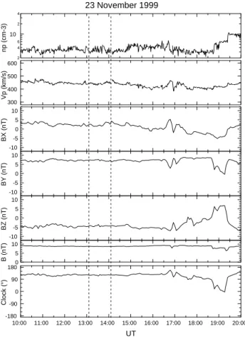
Figure 4 2 4 6 10 2 4 n p ( c m -3 ) 600 500 400 300 V p ( k m /s ) -10 -5 0 5 10 B X ( n T ) -10 -5 0 5 10 B Y ( n T ) -10 -5 0 5 10 B Z ( n T ) 23 November 1999 -180 -90 0 90 180 C lo c k ( °) 10:00 11:00 12:00 13:00 14:00 15:00 16:00 17:00 18:00 19:00 20:00 UT 10 5 0 B ( n T )
Fig. 4. Solar wind (proton) and interplanetary magnetic field data for 23 November 1999 from the ACE spacecraft. Vertical dashed lines show the period of time at ACE that corresponds to the solar wind at Earth during the 14:00–15:00 UT interval analyzed here.
look AE varied between about 400 and 600 nT. Polar UVI auroral images of ∼8 h in MLT centered on midnight (not presented here) are available during this interval and show that there were no auroral substorm intensifications during 14:00–15:00 UT and that the nightside auroral pattern was stable with a double oval in the late evening.
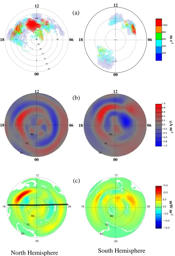
The Doppler velocities from SuperDARN, FACs from the Iridium magnetometer data and S|| for 14:00–15:00 UT, on
23 November 1999, are shown in Fig. 5. For this interval, the SuperDARN convection maps were available for both Northern and Southern (late spring) Hemispheres, giving an indication of conjugate Poynting flux. Figure 5a shows the averaged velocities from the SuperDARN data. Most of the experimental data for the Northern Hemisphere comes from the dayside, with the statistical model completing the night side global estimates. This should be reasonable given the remarkably steady IMF conditions, as shown in Fig. 4. Large flow vectors near 72◦ during mid afternoon indicate enhanced electric fields in this region. The experimental data for the Southern Hemisphere is concentrated around pre-noon and pre-midnight. The statistical model values from the Northern Hemisphere were mapped to the south for estimat-ing the electric fields where there were no radar returns.
Table 3. Locations of the maximum and minimum FACs, and the maximum downward Poynting flux for regions of enhanced Poynt-ing flux for 14:00–15:00 UT, 23 November 1999 (cf. Fig. 5c).
MLAT MLT J||, S|| (deg) (hour) N: 13:00–18:00 MLT Region 1 75 17.0 0.9 µAm−2 Region 2 69 15.0 −0.5 µAm−2 Poynting flux 72† 14.5 13 mWm−2 S: 06:00–09:00 MLT: Region 1 78 8.0 −1.0 µAm−2 Region 2 70 9.0 +0.7 µAm−2 Poynting flux 72 7.5 7 mWm−2 S: 09:00–13:00 MLT: Region 0 (?) 79 12.3 −0.5 µAm−2 Poynting flux 80 11.0 6 mWm−2 S: 13:00–18:00 MLT: Region 1 73 15.0 +1 µAm−2 Region 2 67 14.0 −0.5 µAm−2 Poynting flux 70 16.0 7 mWm−2
† Bold face indicates Poynting flux results within regions of Super-DARN returns.
Figure 5b shows FACs obtained from the Iridium magne-tometer data. For the Northern Hemisphere, the dawnside downward Region 1 currents (blue) merge with the duskside Region 2 currents, a feature that we have found to occur for positive IMF By. The afternoon upward Region 1 current
(red) is the largest in the Northern Hemisphere, peaking at 0.9µAm−2 around 17:00 MLT (see Table 3). The South-ern Hemisphere is viewed through the Earth from the North Pole. Positive current (red) flows radially outward from the southern ionosphere. For the Southern Hemisphere, the af-ternoon Region 1 (red, outward) and Region 2 (blue, inward) currents are clearly defined. The Southern Hemisphere after-noon Region 1 current is contiguous with the morning Re-gion 2 current. This is in approximate mirror symmetry with the Northern Hemisphere.
The spatial distribution of S|| for both hemispheres is
shown in Fig. 5c, and the locations and properties of the cur-rents and S||in regions of enhanced flux are listed in Tables 3
and 4. In the Southern Hemisphere the enhanced Poynt-ing flux region near 07:00 MLT and 72◦is within the area of radar returns associated with large convection velocities there. The region of strong Poynting flux in the north at 15:00 MLT is within the area covered by radar returns, in-dicating narrow latitudinal heating. The enhanced S||regions
that overlap radar returns are indicated in Tables 3 and 4 by bold face type. The most prominent feature in the north is an enhancement of downgoing flux around mid afternoon and
m s -1 A m -2 m W m -2 -90 0 90 180 60 65 70 75 80 85 90 Binned 11/23/1999 14:00:00 -15:00:00 UT 2000 m/s 0 180-90 -70 Binned m/s 11/23/1999 14:02:00 -15:00:00 UT 2000 m/s
North Hemisphere
South Hemisphere
Figure 5
(c)
(b)
(a)
00 06 12 18 00 06 12 18 00 06 12 18 00 06 12 18Fig. 5. Iridium and SuperDARN data averaged over 14:00–15:00 UT, 23 November 1999 for both Northern and Southern Hemispheres.
(a) Plasma velocities from SuperDARN, (b) Field-aligned currents derived from the Iridium magnetometer data. Radial outward (inward) currents are red (blue). (c) Poynting flux and DMSP F-13 track over the Northern Hemisphere.
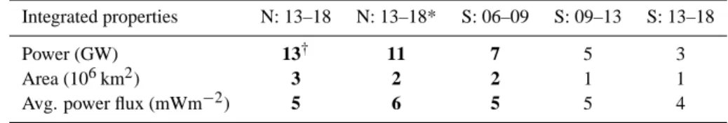
Table 4. Integral properties for four regions of enhanced Poynting flux for 14:00–15:00 UT, 23 November 1999. Integrated power density
extends down to a contour of 2.5 mWm−2in Figure 5c, except as noted.
Integrated properties N: 13–18 N: 13–18* S: 06–09 S: 09–13 S: 13–18
Power (GW) 13† 11 7 5 3
Area (106km2) 3 2 2 1 1
Avg. power flux (mWm−2) 5 6 5 5 4
* Integrals to a contour of 4 mWm−2for comparison with Table 2.
† Bold face indicates Poynting flux results within regions of SuperDARN returns.
in the morning, between the Region 1 and 2 currents. The Poynting flux integrated from 60◦to the pole is 46 GW for both the Southern and Northern Hemispheres.
The regions of enhanced S|| in Fig. 5 account for roughly
one-quarter of the total energy flux. The power levels in these regions and the minima between them were somewhat lower than the event in Fig. 2, so we used a contour at 2.5 mW/m2to evaluate integral properties of the enhancements. The result for the Northern Hemisphere enhancement around 15:00 UT (Fig. 5c), with a contour at 4 mW/m2, is also given for com-parison with the 11 March 2000 case. In the north, the single rather large region of strong S|| accounts for ∼25% of the
total while in the south the two auroral zone enhancements account for ∼20% of the Southern Hemisphere power. Three of the four enhancements occur between the Region 1 and 2 currents (N: 15:00 MLT, S: 08:00 MLT and S: 16:00 MLT). The fourth, S :11:00 MLT, lies poleward of all the resolved major current systems. At 11:00 MLT there are three current “sheets”, so we identify the upward current there as Region 0. Once again, an independent measure of the magnetic field and S|| values is available from DMSP data. For 23
Novem-ber 1999, DMSP F-13 passed 60◦ geomagnetic latitude at 18.0 MLT and tracked across to 60◦ at 06:00 MLT, a dusk to dawn pass. The perturbation magnetic field data obtained along the DMSP F-13 track are compared with the Iridium derived magnetic field data in the top two panels of Fig. 6. The enhanced east-west component magnetic field values from Iridium on the dusk side near 14:50 UT are in good agreement with the DMSP-13 values while the dawn side values near 15:04 UT are underestimated. The median er-rors are 40 nT for the north-south and 30 nT for the east-west component magnetic field data.
The two lower panels in Fig. 6 show the S|| comparison
for data sampled along the DMSP F-13 track (see Fig. 5c) for 23 November 1999. There is general agreement between the two data sets, as shown by the S|| difference histogram
in the lower right panel of Fig. 6. The largest differences are located where DMSP encounters large values of S|| that
occur over small spatial scales. The median error between the two S||data sets is 1.4 mWm−2.
3.3 Integral energy flux: Latitude and local time
Quantitative trends with latitude and local time are difficult to judge from the color maps, so we integrated the S||
distri-butions shown in Figs. 2c and 5c in two ways. To investigate the local time distribution of auroral zone Poynting flux we integrated S|| over latitudes from 64◦ to 75◦ and expressed
the result as power per MLT hour. This is shown for the three cases in Fig. 7. In all cases the smallest power is seen near midnight and noon, and reaches several GW/MLT-hour within a few hours of dawn and dusk. The maxima are fairly broad being four to six hours in extent at half maximum.
There is some evidence for a morning/evening asymme-try. For the 23 November case, the Northern Hemisphere integrated power in the evening is nearly twice that in the morning, whereas in the south they are approximately the same. For 11 March, the power in the morning and evening are essentially the same. Almost all of the asymmetry for the 23 November Northern Hemisphere is due to the large S||
enhancement in the afternoon. Since the IMF By was
posi-tive for 23 November, this local time asymmetry may be due to the asymmetries in reconnection driven convection associ-ated with the IMF By. The asymmetry is not evident in the
Southern Hemisphere for 23 November, indicating that the dynamics in the Northern and Southern Hemispheres may be different. However, there are strong FACs in the South-ern Hemisphere aftSouth-ernoon, so an absence of radar returns, where the statistical data is used may be suppressing any large S|| there. Morning afternoon asymmetries have been
reported in particle precipitation and auroral emissions. For the Northern Hemisphere, particle precipitation and auroral luminosity, on average, exhibit a prominent afternoon “hot spot” (Evans, 1985; Newell et al., 1996a; Liou et al., 1997b), whereas a morning enhancement associated with positive Bz
is comparatively weak (Newell et al., 1996a).
To examine the relative importance of power incident in the auroral zone to that over the polar cap we integrated the S||over local time to obtain the power per unit latitude,
dP /dλ=R S||(λ, ϕ)rcos(λ)dϕ, and then calculated the
cu-mulative power equatorward of λ, P(λ), by integrating dP/dλ from 60◦to λ◦. The cumulative power for the 11 March 2000 interval and both hemispheres for the 23 November 1999 in-terval are shown in Fig. 8. (The Southern Hemisphere is
Figure 6
Fig. 6. Comparison of Northern Hemisphere DMSP F-13 data with Iridium/SuperDARN values for 23 November 1999. (top panels) DMSP F-13 and Iridium derived magnetic field values in north-south (left panel) and east-west (right panel) components. (lower panels) Poynting flux data along the DMSP track from 18.0 to 6.0 MLT (left panel) and a histogram of the differences in Poynting flux (right panel).
Table 5. Total power in the auroral zone, divided into 00:00–12:00 (AM) and 12:00–24:00 (PM) local time ranges, and total polar cap power.
Aur 00:00–12:00 MLT Aur 12:00–24:00 MLT Aur AM/PM Polar Cap 75◦–90◦
(GW) (GW) (GW)
N: 11 March 2000 19 15 1.3 14
N: 23 November 1999 10 17 0.6 16
S: 23 November 1999 12 12 1 19
shown versus |λ|.) For all three cases, the latitudes where P(λ) is the steepest are about 65◦ to 75◦. Poleward of 75◦,
P(λ) continues to rise, indicating power incident over the po-lar cap.
The total polar cap power, the total auroral zone power and the auroral zone power in the morning and evening for the three cases are listed in Table 5. We used 64◦-75◦ and 75◦–90◦for the auroral and polar cap latitude ranges, respec-tively. The auroral zones account for most of the total power,
∼60−70%, on average. For all three cases the total power incident over the polar cap is a significant fraction of the to-tal, ∼40% for both hemispheres on 23 November and ∼30% for 11 March. Therefore, even though S|| peaks in the
au-roral zone, the energy flux into the polar cap is a significant portion, about 1/3, of the total power budget.
4 Discussion
We have presented measurements of the global distribution of net Poynting flux linking the high-latitude ionosphere and magnetosphere on one-hour time scales. This has been achieved without estimating parameters such as ionospheric conductivities, neutral wind velocities or ion collision fre-quencies. The Poynting flux reported here is the net elec-tromagnetic energy density linking the thermosphere, iono-sphere and magnetoiono-sphere. The physical processes involved in the energy exchange are readily seen from Eq. (2). The first term on the RHS gives the rate at which electrical en-ergy is converted to heating the neutral gas while the second term describes the conversion from mechanical to electrical energy (Thayer and Vickrey, 1992; Richmond and Thayer, 2000). Usually, the J ×B force acts to accelerate the neutral wind, but this term can be negative, in which case mechani-cal energy is converted to electrimechani-cal energy corresponding to
Figure 7
4 3 2 1 0 G W /M L T -h o u r 11 Mar 2000 1600-1700UT 4 3 2 1 0 G W /M L T -h o u r 24 18 12 6 0 MLT N S 23 Nov 1999 1400-1500UTAuroral Zone Power: 65°-75° MLAT
Fig. 7. Auroral zone power in GW per hour of MLT versus local time for (top) 11 March 2000 and (bottom) 23 November 1999.
Poynting flux was integrated over 64◦–75◦geomagnetic latitude.
the “flywheel” effect (Lyons et al., 1985). The Poynting flux in Figs. 2c and 5c is the combined effect of these processes.
The results for the events presented in Figs. 2 and 5 have integrated powers of ∼50 GW, with maximum S||around 10
to 15 mWm−2. Peak values of S||are underestimated to a
de-gree that increases as the spatial structure narrows due to the spatial resolution of the Iridium magnetic perturbation maps. The data fitting process will smooth and reduce the magnetic field estimates in these regions. If we allow for an under-estimate in S|| of ∼30% in the auroral zone, the integrated
powers over 60◦to the pole reach ∼60 GW. This total energy flux is on the smaller side of typical passive heating rates obtained by the AMIE procedure, which are typically 50 to 100 GW for non-storm times (e.g. Lu et al., 1996; Buonsanto et al., 1999; Slinker et al., 1999).
The Joule heating values provided by AMIE is indirect and subject to two primary sources of uncertainty. First, the in-ferred electric fields and ionosphere currents depend on es-timates of Hall and Pedersen conductivities. Comparison under different conductivity assumptions show that the re-sults are sensitive to the conductivities (e.g. Richmond et al., 1990). The conductivity distributions are estimated by mod-ifying statistical models using correlations between ground magnetic signals and conductivity (Ahn et al., 1983), low Earth orbit particle precipitation data and UV auroral emis-sion images when available. While the energy flux can be estimated from auroral UV images (Lummerzheim et al., 1997), the conductivities depend on the energy spectrum
Figure 8
50 40 30 20 10 0 P o w e r (G W ) 11 Mar 2000 1600-1700UT 50 40 30 20 10 0 P o w e r (G W ) 90 85 80 75 70 65 60 MLAT (°) 23 Nov 1999 1400-1500UT N S Cumulative PowerFig. 8. Cumulative power integrated over local time in 2◦MLAT bins versus magnetic latitude for (top) 11 March 2000 and (bottom) 23 November 1999.
which must be estimated by comparing two bands in the UV (Germany et al., 1994). The uncertainties in the resultant es-timated conductivity distributions and their contributions to the errors in the derived Joule heating rates are difficult to characterize.
The second source of uncertainty is that the Joule heating rates calculated by AMIE are the passive energy dissipation
Qj*. Radar experiments (Fujii et al., 1999; Thayer, 2000)
and simulations (Lu et al., 1995) indicate that Qj* typically
overestimates Qj by 10−30%. The disparity between Qj*
and J ·E is often larger by a factor of two during moderate activity (Fujii et al., 1999; Thayer, 2000). Therefore, the estimates of Joule heating provided by AMIE depend on as-sumptions whose quantitative effect on the results can be dif-ficult to judge but which are probably significant, particularly if one is interested in the net energy dissipation.
Our total auroral zone energy flux is also smaller than the 84-GW average passive heating power determined using EISCAT and SABRE over the latitude range observed by the radars (Kosch and Nielsen, 1995). This is not entirely un-expected since the passive heating rate is usually an overes-timate of the net electromagnetic energy flux (Thayer, 1998, 2000). The maximum S||is comparable to those from the ISR
experiments though somewhat lower than maxima obtained by single spacecraft (Kelley et al., 1991; Gary et al., 1995). We find that Poynting flux in the auroral zones is not uniform with local time but tends to maximize in “hot spots” whose location and extent differs between hemispheres and appear
to depend on the IMF. Local time structuring in the passive heating rate estimates from AMIE is also typical (Lu et al., 1996; Slinker et al., 1999). Given that both techniques obtain structured energy distributions at auroral latitudes suggests that it should be easy to test whether these localized heating regions match in future intercomparisons.
A new feature reported here is that the Poynting flux over the polar cap is an appreciable fraction of the total electro-magnetic energy. The total net energy flux poleward of the large-scale current systems accounts for up to half as much as the total auroral zone input. Deng et al. (1995), using DE-2, found that the Poynting flux over the polar cap was a significant fraction of that occurring in the auroral zones. The electric and magnetic fields are approximately uniform over the polar cap. This implies that the corresponding J ×B force in the ionosphere is fairly horizontally uniform over the entire polar cap, providing an anti-sunward neutral wind flow with a scale size larger than the latitudinal extent of the auro-ral zones (Thayer et al., 1995). Simulations of neutauro-ral wind velocities show similar large-scale flows (Lu et al., 1995) and indicate that polar cap electromagnetic energy flux is dis-sipated largely by neutral wind acceleration (Thayer et al., 1995).
The large-scale pattern of energy flux in Fig. 2c with max-ima in the morning and evening is qualitatively different from the average distribution of particle energy flux. Statistical studies of both auroral particle precipitation (Hardy et al., 1989; Newell et al., 1996a) and auroral luminosity (Liou et al., 1997b; Shue et al., 2001) found broad maxima on the nightside with a lower flux on the dayside and very low de-position over the polar cap. A similar difference, with precip-itation energy flux stronger on the nightside and Joule heat-ing stronger on the dayside, was observed for a geomagnetic storm (Anderson et al., 1998). Since S|| often maximizes on
the dayside, it appears that field-aligned currents and their concomitant energy density flow are not necessarily corre-lated with auroral luminosity. This is consistent with statis-tical studies of Newell et al. (1996b) and Liou et al. (2001), who showed that aurora and precipitating particle energy flux are more prevalent for the nighttime ionosphere. The dif-ference between auroral and S|| distributions indicates that
particle and electromagnetic energy flux are somewhat com-plementary.
One aspect of the Poynting flux results has an interesting parallel with auroral emissions and particle precipitation. A number of statistical studies have reported preferred regions of enhanced auroral activity known as “hot” or “warm” spots (Cogger et al., 1977; Evans, 1985; Newell et al., 1996a; Liou et al., 1997a). On average, a hot spot is located be-tween 14:00–16:00 MLT and appears to correspond with Re-gion 1 FAC latitudes. From a statistical analysis of 9 years of electron acceleration events in DMSP data, Newell et al. (1996a) showed that for northward directed IMF, a less intense “warm” spot can occur between 06:00–09:00 MLT. With the ability to map global Poynting flux on relatively short time scales, hot spots can now be identified in terms of electromagnetic energy flux. Figure 2c shows large
down-ward Poynting flux around dawn, in the warm spot MLT sector reported in Newell et al. (1996a) but for southward IMF. Figure 5c shows enhanced downward Poynting flux during mid afternoon and near Region 1 FACs for the North-ern Hemisphere, in good agreement with previous observa-tions of the afternoon hot spot. These events suggest that, on an individual basis, distinct, heated regions may develop for southward IMF conditions and the previously statistically identified morning warm spot may on occasion contain the larger Poynting flux. Future investigations of the relationship between the global Poynting flux and particle precipitation enhancements should reveal how dayside enhanced auroral regions are related to Poynting flux and the field-aligned cur-rents.
There have been reports of negative (upward) Poynting flux (e.g. Gary et al., 1995). This may occur where the me-chanical energy term is larger than the Joule heating term in Eq. (2) and the neutral gas, through U, drives the mag-netosphere. The contours of zero Poynting flux in Figs. 2c and 5c are highlighted in white. Within these areas there are hints of upward Poynting flux. These occur at the pole-ward side of the Region 1 currents, consistent with previ-ous results that upward Poynting flux tends to occur near the ionospheric plasma convection reversal (Kelley et al., 1991; Gary et al., 1995). Regions of upward Poynting flux driven by neutral winds are also predicted by thermosphere circula-tion models (Thayer and Vickrey, 1992; Thayer et al., 1995). However, since the convection reversal is where the mag-netic perturbations reverse it is also where uncertainties in the measured magnetic field perturbations have the largest relative effect and the direction of the magnetic perturbation is uncertain, and hence so is the sign of S||. The Iridium
mag-netometer data have 48 nT resolution commensurate with the median differences with the DMSP magnetometer perturba-tions. Comparison with other LEO satellite magnetometer data in these regions is necessary to confidently identify up-ward Poynting flux. For the moment, uncertainties in fitted data are large enough to introduce significant errors in the location of the null point in the magnetic field perturbation. The Doppler velocity and hence electric field estimates also have uncertainties, although they may be smaller than for the magnetic field data. In regions where there are no radar re-turns, the electric fields are derived from a statistical model based on IMF orientation. While choosing steady IMF in-tervals may be more likely to bring the actual values near those estimated from the statistical model, the relative errors will be largest near the convection reversal. Therefore, we do not regard the results presented here as confirming the oc-currence of upward Poynting flux. Nonetheless, using the approach presented here, it may be possible in the future to identify Poynting flux, driven by the neutral wind dynamo, following transitions from sustained forced convection to lit-tle or no magnetospheric forcing (Deng et al., 1991; 1993; Asamura and Iyemori, 1995).
5 Conclusions
We have developed a new technique to estimate the elec-tromagnetic energy flux at the topside ionosphere. The method employs global-scale measurements of plasma drift from the SuperDARN radars to estimate electric fields and magnetic field measurements from the >70 Iridium polar orbiting satellites, to estimate the magnetic perturbations at high latitudes. The electric and magnetic fields are then represented by spherical harmonic functions and their cross product yields the Poynting flux directly from first principles. For the two events analyzed here we compared the re-sults against independent Poynting flux determinations from low Earth orbiting satellites. The DMSP drift meter and magnetometer data allow us to estimate the local Poynting flux along the satellite track, and one track was available with suitable data for each event. We evaluated our two-dimensional map for the Poynting flux along the satellite track to compare directly with the DMSP results. We find general agreement both in the co-location of maximum fluxes and in the quantitative values to within a few mW/m2. The agreement is consistent with the 2◦ MLAT and 2-h MLT resolution of the perturbation magnetic field fit to the Irid-ium data, that is, our distribution is smoothed relative to the DMSP results.
There are two principal limitations to the technique as im-plemented. Because it presently takes approximately 1 h to accumulate sufficient samples from the Iridium constellation, the technique is applicable to situations for which convec-tion and solar wind forcing are stable over this time scale. Even with this limitation, the technique reduces the time to construct the distribution of high-latitude Poynting flux from many months to just one hour. This allows us to determine the Poynting flux distribution for specific events as opposed to the long-term averages from single satellites that were available previously. Second, the electric field estimates are most reliable in regions where radar returns were obtained and hence where Doppler velocity measurements were made. Elsewhere, the electric field estimates are driven by statistical patterns. The results are therefore most reliable in regions of radar returns and since this is known, regions of higher and lower reliability are readily identified.
The SuperDARN/Iridium approach offers two primary ad-vantages that complement other techniques used to estimate high-latitude energy input. First, because the technique yields the net electromagnetic energy flux directly, the in-fluence of the neutral winds is included. Comparisons with techniques that yield the net Joule dissipation using incoher-ent scatter radars may allow independincoher-ent assessmincoher-ent of the neutral wind contribution to energy transport. Second, be-cause the approach does not require any assumptions regard-ing ionosphere conductivities, it can provide an independent test of techniques which rely on ground magnetometer data to infer electric fields and energy dissipation.
These first analyses yield two new results on the distribu-tion of Poynting flux at high latitudes. First, the Poynting flux over the polar cap, poleward of Region 1, is approximately
1/3 of the total, or about 15 GW in the two cases presented here. Since the electric and magnetic fields were mately uniform over the polar cap, this implies an approxi-mately uniform anti-sunward J ×B force accelerating neu-tral winds. This result is consistent with Deng et al. (1995) and suggests that the neutral wind dynamo may play a role in electrodynamics on the nightside, where the inertia of the neutral wind carries it through the nightside auroral zone as suggested by the modeling results of Thayer et al. (1995). Second, we find that the auroral zone Poynting flux can be rather concentrated in a few, two to three, hours of local time. These regions of enhanced Poynting flux may be related to the regions of enhanced auroral activity known as “hot” or “warm” spots (Cogger et al., 1977; Evans, 1985; Newell et al., 1996a; Liou et al., 1997b). In general, the auroral zone Poynting fluxes maximize near dawn and dusk in contrast to statistical distributions of auroral emissions which maximize at night. Comparison of Poynting flux distributions as ob-tained here with auroral imagery will allow us to assess the simultaneous distribution of the particle and electromagnetic energy inputs and determine the relationships between them. Acknowledgements. Work performed at The Johns Hopkins Uni-versity Applied Physics Laboratory was supported by NSF under Grants ATM-0101064 and ATM-9812078. We gratefully acknowl-edge the following investigators who provided solar wind, inter-planetary magnetic field, auroral imaging, and geosynchronous par-ticle data for this study: K. Ogilvie at NASA GSFC for provid-ing WIND solar wind data (via CDAWeb); G. Parks of the Univer-sity of California at Berkeley for providing the Polar UVI image data (via CDAWeb); D. J. McComas of SwRI for providing ACE solar wind/proton data (via the ACE project); N. Ness of Bartol Research Institute for providing ACE interplanetary magnetic field data (via the ACE project); T. Kamei of the Kyoto World Data Cen-ter for providing the quicklook AE indices. We gratefully acknowl-edge F. Rich of the Air Force Research Laboratory for providing the DMSP Special Sensor Magnetometer (SSM) data and thermal plasma data from the Special Sensor-Ions, Electrons, and Scintil-lation (SSIES) package and M. Hairston for providing analysis of the drift meter and ion retarding potential analyzer portions of the SSIES data.
Topical Editor M. Lester thanks two referees for their help in evaluating this paper.
References
Ahn, B.-H., Robinson, R. M., Kamide, Y., and Akasofu, S.-I.: Elec-tric conductivities, elecElec-tric fields and auroral energy injection rate in the auroral ionosphere and their empirical relations to the horizontal magnetic disturbances, Planet Space Sci., 31, 641, 1983.
Anderson, B. J., Gary, J. B., Potemra, T. A., Frahm, R. A., Sharber, J. R., and Winningham, J. D.: UARS observations of Birkeland currents and Joule heating rates for the November 4, 1993 storm, J. Geophys. Res., 103, 26 323–26 335, 1998.
Anderson, B. J., Takahashi, K., and Toth, B. A.: Sensing global Birkeland currents with Iridium engineering magnetometer data, Geophys. Res. Lett., 27, 4045, 2000.
Anderson, B. J., Takahashi, K., Kamei, T., Waters, C. L., and
de-rived from Iridium observations: Method and initial valida-tion results, J. Geophys. Res., 107, A6, SMP 11-1-11-13, 10.1029/2001JA000080, 2002.
Anderson, B. J., Christiansen, F., Waters, C. L., Papitashvilli, V.: Intercomparison of Iridium derived magnetic perturbation maps with Oersted observations, XXIII General Assembly of IUGG, Sapporo, 2003.
Asamura, K. and Iyemori, T.: Flywheel effect deduced from geo-magnetic variation in the polar region, J. Geomagn. Geoelectr., 57, 973–987, 1995.
Baker, K. B. and Wing, S. A.: New magnetic coordinate system for conjugate studies at high latitudes, J. Geophys. Res., 94, 9139, 1989.
Buonsanto, M. J., Gonzalez, S. A., Lu, G., Reinisch, B. W., and Thayer, J. P.: Coordinated incoherent scatter radar study of the January 1997 storm, J. Geophys. Res., 104, 24 625–24 637, 1999. Cogger, L. L., Murphree, J. S., Ismail, S., and Anger, C. D.:
Char-acteristic of dayside 5577 ˚A and 3914 ˚A aurora, Geophys. Res.
Lett., 4, 413, 1977.
Cole, K.D.: Joule heating of the upper atmosphere, Aust. J. Phys., 15, 223, 1962.
Cole, K. D.: Energy deposition in the thermosphere caused by the solar wind, J. Atmos. Terr. Phys., 37, 939, 1975.
Deng, W., Killeen, T. L., Burns, A. G., and Roble, R. G.: The fly-wheel effect – Ionospheric currents after a geomagnetic storm, Geophys. Res. Lett., 18, 1845–1848, 1991.
Deng, W., Killeen, T. L., Burns, A. G., Roble, R. G., Slavin, J. A., and Wharton, L. E.: The effects of neutral inertia on ionospheric currents in the high-latitude thermosphere following a geomag-netic storm, J. Geophys. Res., 98, 7775–7790, 1993.
Deng, W., Killeen, T. L., Burns, A. G., Johnson, R. M., Emery, B. A., Roble, R. G., Winningham, J. D., and Gary, J. B.: One-dimensional hybrid satellite track model for the Dynamics Ex-plorer 2 (DE 2) satellite, J. Geophys. Res., 100, 1611–1624, 1995.
Evans, D. S.: The characteristics of a persistent auroral arc at high latitudes in the 1400 MLT sector, in: The Polar Cusp, edited by Holtet, J. and Egeland, A., D. Reidel Publishing Company, Norwell, Mass., 99–109, 1985.
Foster, J. C., Maurice, J.-P. St., and Abreu, V. J.: Joule heating at high latitudes, J. Geophys. Res., 88, 4885, 1983.
Fujii, R., Nozawa, S., Matuura, N., and Brekke, A.: Study on neu-tral wind contribution to the electrodynamics in the polar iono-sphere using EISCAT CP-1 data, J. Geophys. Res., 103, 14 731– 14 739, 1998.
Fujii, R., Nozawa,S., Buchert, S. C., and Brekke, A.: Statistical characteristics of electromagnetic energy transfer between the magnetosphere, the ionosphere, and the thermosphere, J. Geo-phys. Res., 104. 2357–2365, 1999.
Gary, J. B., Heelis, R. A., and Thayer, J. P.: Summary of field-aligned Poynting flux observations from DE 2, Geophys. Res. Lett., 22, 1861, 1995.
Germany, G. A., Torr, D. G., Richards, P. G., Torr, M. R., and John, S.: Determination of ionospheric conductivities from FUV auro-ral emissions , J. Geophys. Res., 99, 23 297–23 305, 1994. Greenwald, R. A., Baker, K. B., Hutchins, R. A., and Hanuise, C.:
An HF phased-array radar for studying small-scale structure in the high-latitude ionosphere, Radio Sci., 20, 63, 1985.
Greenwald, R. A., Baker, K. B., Dudeney, J. R., Pinnock, M., Jones, T. B., Thomas, E. C., Villain, J.-P., Cerisier, J.-C., Senior, C., Hanuise, C., Hunsucker, R. D., Sofko, G., Koehler, J., Nielsen, E., Pellinen, R., Walker, A. D. M., Sato, N., and Yamagishi, Y.:
DARN/SuperDARN: A global view of high-latitude convection, Space Sci Rev., 71, 763, 1995.
Hardy, D. A., Gussenhoven, M. S., and Brautigam, D.: A statistical model of auroral ion precipitation, J. Geophys. Res., 94, 370– 392, 1989.
Heelis, R. A. and Coley, W. R.: Global and local joule heating ef-fects seen by DE 2, J. Geophys. Res., 93, 7551, 1988.
Kamide, Y., Richmond, A. D., and Matsushita, S.: Estimation of ionospheric electric fields, ionospheric currents, and field-aligned currents from ground magnetic records, J. Geophys. Res., 86, 801–813, 1981.
Kelley, M. C., Knudsen, D. J., and Vickrey, J. F.: Poynting flux measurements on a satellite: A diagnostic tool for space research, J. Geophys. Res., 96, 201, 1991.
Kosch, M. J. and Nielsen, E.: Coherent radar estimates of average high-latitude ionospheric Joule heating, J. Geophys. Res., 100, 12 201–12 215, 1995.
Liou, K., Newell, P. T., Meng, C.-I., and Lui, T. Y.: Dayside auro-ral activity as a possible precursor of substorm onsets: A survey using Polar ultraviolet imagery, J. Geophys. Res., 102, 19 835, 1997a.
Liou, K., Newell, P. T., Meng, C.-I., Brittnacher, M., and Parks, G.: Synoptic auroral distribution: A survey using Polar ultraviolet imagery, J. Geophys. Res., 102, 27 197–27 206, 1997b.
Liou, K., Newell, P. T., and Meng, C.-I.: Seasonal effects on auro-ral particle acceleration and precipitation, J. Geophys. Res. 106, 5531–5542, 2001.
Lu, G., Richmond, A. D., Emery, B. A., and Roble, R. G.:
Magnetosphere-ionosphere-thermosphere coupling: Effect of
neutral winds on energy transfer and field-aligned current, J. Geophys. Res., 100, 19 643–19 659, 1995.
Lu, G., Emery, B. A., Roger, A. S., Lester, M., Taylor, J. R., Evans, D. S., Ruohoniemi, J. M., Denig, W. G., de la Beaujardiere, O., Frahm, R. A., Winningham, J. D., and Chenette, D. L.: High-latitude ionosphere electrodynamics as determined by the assim-ilative mapping of ionospheric electrodynamics procedure for the conjunctive SUNDIAL/ATLAS 1/GEM period of March 28-29, 1992, J. Geophys. Res., 101, 26 697–26 718, 1996.
Lu, G., Baker, D. N., McPherron, R. L., Farrugia, C. J., Lum-merzheim, D., Ruohoniemi, J. M., Rich, F. J., Evans, D. S., Lep-ping, R. P., Brittnacher, M., Li, X., Greenwald, R. A., Sofko, G., Villain, J., Lester, M., Thayer, J. P., Moretto, T., Milling, D., Troshichev, O., Zaitzev, A., Odintzov, V., Makarov, G., and Hayashi, K.: Global energy deposition during the January 1997 magnetic cloud event, J. Geophys. Res., 103, A6, 11 685, 1998. Lummerzheim, D., Brittnacher, M., Evans, D., Germany, G. A.,
Parkes, G. K., Rees, M. H. and . Spann, J. F: High time resolution study of the hemispheric power carried by energetic electrons into the ionosphere during the May 19/20, 1996 auroral activity, Geophys. Res. Lett., 24, 987, 1997.
Lyons, L. R., Killeen, T. L., and Walterscheid, R. L.: The neutral wind “flywheel” as a source of quiet-time, polar-cap currents, Geophys. Res. Lett., 12, 101, 1985.
Newell, P. T., Lyons, K. M., and Meng,C.-I.: A large survey of electron acceleration events, J. Geophys. Res., 101, 2599, 1996a. Newell, P. T., Meng, C.-I., and Lyons, K. M.: Suppression of
dis-crete aurorae by sunlight, Nature, 381, 766, 1996b.
Rees, M. H., Lummerzheim, D., Roble, R. G., Winningham, J. D., and Craven, J. D.: Auroral energy deposition rate, characteristic electron energy, and ionospheric parameters derived from Dy-namics Explorer 1 images, J. Geophys., Res., 93, 12 841, 1988. Richmond, A. D. and Kamide, Y.: Mapping electrodynamic
fea-tures of the high-latitude ionosphere from localized observations: Technique, J. Geophys. Res., 93, 5741, 1988.
Richmond, A. D., Kamide, Y., Akasofu, S.-I., Alcayde, D., Blanc, M., de la Beaujardiere, O., Evans, D. S., Foster, J. C., Friis-Christensen, E., Holt, J. M., Pellinen, R. J., Senior, C., and Za-itzev, A. N.: Global measures of ionospheric electrodynamic activity inferred from combined incoherent scatter radar and ground magnetometer observations, J. Geophys. Res., 95, 1061– 1071, 1990.
Richmond, A. D. and Thayer, J. P.: Ionospheric dynamics: A tu-torial, in: Magnetospheric Current Systems, Geophys. Monogr. 118, edited by Ohtani, S., Fujii, R., Hesse, M., and Lysak, R. L., AGU, 2000.
Ruohoniemi, J. M. and Baker, K. B.: Large-scale imaging of high-latitude convection with Super Dual Auroral Radar Network HF radar observations, J. Geophys. Res., 103, 20 797, 1998. Ruohoniemi, J. M. and Greenwald, R. A.; Statistical patterns of
high-latitude convection obtained from Goose Bay HF radar ob-servations, J. Geophys. Res., 101, 21 743, 1996.
Shepherd, S. G. and Ruohoniemi, J. M.: Electrostatic potential pat-terns in the high-latitude ionosphere constrained by SuperDARN measurements, J. Geophys., Res., 105, 23 005, 2000.
Shue, J.-H., Newell, P. T., Liou, K., and Meng, C.-I.: Influence of interplanetary magnetic field on global auroral patterns, J. Geo-phys. Res., 106, 5913–5926, 2001.
Slinker, S. P., Fedder, J. A., Emery, B. A., Baker, K. B., Lum-merzheim, D., Lyon, J. G., and Rich, F. J.: Comparison of global MHD simulations with AMIE simulations for the events of 19– 20 May , 1996, J. Geophys. Res., 104, 28 379, 1999.
Thayer, J. P. and Vickrey, J. F.: On the contribution of the thermo-spheric neutral wind to high-latitude energetics, Geophys. Res. Lett., 19, 265, 1992.
Thayer, J. P., Vickrey, J. F., Heelis, R. A., and Gary, J. B.: Interpre-tation and modeling of the high-latitude electromagnetic energy flux, J. Geophys. Res., 100, 19 715–19 728, 1995.
Thayer, J. P.: Height-resolved Joule heating rates in the high-latitude E region and the influence of neutral winds, J. Geophys. Res., 103, 471, 1998.
Thayer, J. P.: High-latitude currents and their energy exchange with the ionosphere-thermosphere system, J. Geophys. Res., 105, A10, 23 015–23 024, 2000.
Vickrey, J. F., Vondrak, R. R., and Matthews, S. J.: Energy deposi-tion by precipitating particles and joule dissipadeposi-tion in the auroral ionosphere, J. Geophys. Res., 87, 5184, 1982.
Waters, C. L., Anderson, B. J., Liou, K.: Estimation of global field aligned currents using Iridium magnetometer data, Geo-phys. Res. Lett., 28, 2165, 2001.