Discrete visual structures : elements of visual grammar

DISCRETE VISUAL STRUCTURES: Elements of Visual Grammar

by Goran Dordevic

B.E.E Electrotechnical Faculty Belgrade, Yugoslavia

June 1980

Submitted to the Department of Architecture in partial fulfillment of the requirements of the degree of Master of Science in Visual Studies at Massachusetts Institute of Technology

September 1984

@ Goran Dordevic 1984

The author hereby grants to M.I.T permission to reproduce and to

distribute publicly copies of this thesis document in whole or in part.

Signrt re of. Author, G Dordevic, Department of Architecture,

Auk ist I,84//

/'

I

.Aetfied by Muh6l Coopfet, Associate. rof essor of Visual Studies Thesis Supervisor

ed by Nicholas Negroponte, Chair, Departmental Committee for Graduate Students

0F rEHN L y

OCT 0 5 1984

UBFRA RE3

in partial fulfillment of the requirements of the degree of Master of Science in Visual Studies at Massachusetts Institute of Technology

August 10, 1984

Abstract

Is it possible to reason by means of images? If it is, then with what kind of images can we organize thoughts? How can the rules governing the relations between images be established? Could these relations be as complex and productive as those defined within the grammar of the verbal language?

The basic construction of any language, especially a developed one, is a structure of formal rules which regulate the relations between its signs or elements. For verbal language it is a syntax which regulates all relationships between elements of a certain language: alphabet, words and sentences.

This work is an attempt to explore and establish a set of formal rules between a large and complex group of standardized visual signs which I call discrete visual structures. A fundamental characteristic of a discrete visual structure is its possibility to be visually represented. The relations between these structures depend primarily on their graphic organization and structural characteristics. Elements of each structure can be presented as finite parts of the plane surface. There are four basic types of

discrete visual structures: spatial structure, qualitative structure, state of space and

visual process.

I have based this presentation of discrete visual structures on two different types

of signs: visual and verbal. but the visual presentation of images is the essential

subject of this analysis. Verbal signs (written text) are used here as a necessary meta-language in order to communicate the basic ideas on discrete visual structures to the readers.

Thesis Supervisor: Muriel Cooper Associate Professor of Visual Studies

CONTENTS Abstract - _ _ - _ _ _ _ - _ - - - _ - - - - - _ Contents - _ _ _ _ -Introduction _ _ _ Spatial Structure _ _ _ _ _ _ -Qualitative Structure _ _ _ _ _ _ _ _ _ _ _ _ _ State of Space - - - _ _ _ Visual Process _ _ _ _ _ _ -References - - - ---- - - - -- - -- - - - 125 3 5 7 11 33 55 91

INTRODUCTION

Is it possible to reason by means of images? If it is, then with what kind of images can we organize thoughts? How can the rules governing the relations between images be established? Could these relations be as complex and productive as those defined within the grammar of the verbal language?

It is now more than twelve years since I began to be interested in various problems related to a rather unclear and polysemic concept of the visual language. These or similar questions were the roots of my interest which lead me to work on

formal aspects of visual signs developing some manner of visual grammar.

I take language to be primarily a vehicle for thought or selfcommunication. In my

opinion, it is also a window to the world. If we find ourselves in a room without windows, there is no picture of the world. One can say that there is no world at all. Initially, the window was small and sight was limited and poor. Throughout the ages the window became wider, more elements were added, many new colors appeared, and many details were altered and changed. Hence today, through the window of verbal

language we learn to perceive a very complex and sophisticated landscape of the

world. However, since the window is merely a frame and the landscape is simply a

picture, our vision of the world is naturally limited and distorted.

Any new language, based on premises other than verbal language, can open another

window in our room, allowing us to see a different picture of the same world. These

different pictures will give us a much wider and more complex vision of the universe.

I believe that a highly organized and developed visual language provides such a new

window.

The basic construction of any language, especially a developed one, is a structure

of formal rules which regulate the relations between its signs or elements. For verbal

language it is a syntax which regulates all relationships between elements of a certain

language: alphabet, words and sentences.

This work is an attempt to explore and establish a set of formal rules between a

large and complex group of standardized visual signs which I call discrete visual

structures. A fundamental characteristic of a discrete visual structure is its possibility

to be visually represented. The relations between these structures depend primarily on

their graphic organization and structural characteristics. Elements of each structure can

be presented as finite parts of the plane surface. There are four basic types of

discrete visual structures: spatial structure, qualitative structure, state of space and

visual process.

Spatial structure is defined as a structure of position. Each element of this

structure is presented as a definite part of the plane with defined neighborhood

relations with other elements of the same structure, presented in standard form. A

position is a basic characteristic of each element within a spatial structure. Therefore,

any particular spatial structure represents a specific universe of positions with its own

topological integrity.

Qualitative stucture is defined as a structure of content. Each element of this

structure is presented as a definite part of the plane with defined neighborhood

conventional. A natural presentation keeps the natural neighborhood relations between qualities. This means that in a white-gray-black structure, white can be a neighbor of gray but not of black. In a conventional presentation the neighborhood relations can be presented arbitrarily.

State of space is defined as a union of both spatial and qualitative structures. Here we have a complex visual structure with defined both position and content for each element within a structure. With a state of space it is possible to analyze in more detail topological characteristics of a spatial structure and to distinguish various kinds

of figures within a structure. State of space can also be very helpful in analyzing the relations between different qualities. It is shown that some qualities, like gray for example, are not independent and can be generated by uniform distribution of two basic qualities: black and white. Therefore, within a state of space we can get much

more information about both spatial and qualitative structures. A matrix state is a distinct kind of state which represents a visual image of neighborhood relations of a certain spatial structure.

A visual process is defined as appearance of equal or different states of space presented in sequences. The order of appearance of the same or different states of space is a rhythm. With a given number of different states we can generate a random process. In this kind of process it is known what states can appear but the order of their appearance is not predictable. Another group of processes, generated by unar operators, are predictable. since we know the exact order of appearance of same or different states throughout the entire process. by knowing which particular operator is

employed.

I have based this presentation of discrete visual structures on two different types of signs: visual and verbal, but the visual presentation of images is the essential

subject of this analysis. Verbal signs (written text) are used here as a necessary meta-language in order to communicate the basic ideas on discrete visual structures to the readers.

CHAPTER I

SPATIAL STRUCTURE

1.1 Let some finite set be A = (a,b,c,d,e) and let the neighborhood relations between elements of the set be defined in the following way:

a*b, a*d, b*c, b*d, c*d, d*e.

Neighborhood relation is symmetric, which means that a*b.= b*a. If we presume that

the elements of A-set can be presented as definite parts of a plane, with a defined

d

b Fig.1.1

form and size such as those shown in Fig.1.1a, for example, then the observed structure can also be presented in the following way (Fig.1.1b): We can see that the

spatial neighborhood relations of elements in the structure are equal to those given by the relation above. A structure whose elements are definite parts of a plane with

defined spatial neighborhood relations we will name the spatial structure. A set of

elements which can define a spatial structure is the generating set. However, with the

set of elements shown in Fig.1.1a it is possible to present a given structure in a number of ways as shown in Fig.1.2. In order to avoid such polysemic presentation of

a _{c d} d b d e b a d -- ebc b a c a e b Fig.1.2

a spatial structure, we will adopt the form of the structure presented in Fig.1.1b as

the standard form for any spatial structure. Therefore, only the structure presented through such a standard form can be named a spatial structure. In the following text

Fig.1.3

it will be presented as shown in Fig.1.3. At the same time the one-element (monoelement) spatial structure will be presented in this way as well.

1.2 According to the previous explication we have some idea about neighborhood

relations between elements of the spatial structure. For example, in the structure

shown in Fig.1.1b elements (a) and (b) are neighbors, but not elements (a) and (c).

WL

Fig.1.4

E

N-F

Fig.1.5

Therefore, in spatial structure Sa (Fig.1.6), elements (a) and (b) are neighbors but not

elements (a) and (c). In the structure Sb, elements (d) and (e). or (f) and (g) are

neighbors. In the same structure elements (d) and (f) are not neighbors, nor are (e) and (g). In structure Sc element (k) is a neighbor of (h) and (i), but elements (h), (i)

a b d

Fig.1.6

e

and (j) are not mutual neighbors. In structure Sd, for example, elements (1) and (m),

and (1) and (n) are neighbors, but elements (m) and (n) are not. In the last structure (Se), element (p) is a neighbor of (o) and (q), but these elements are not mutual neighbors.

1.3 If we have two different generating sets: A = (a,b,c,d,e) and B = (f,g,h,i,j) with an equal number of elements but with a different form and size, as shown in

I

I I

Fig.1.7a, we can define two different spatial structures (Fig.1.7b). The neighborhood

b d e

-- h i

a b

Fig.1.7

relations between elements of these two spatial structures are:

a*b, a*d, a*c, b*d, c*d, d*e;

f*g, f*i, g*h, g*i, h*i, i*j.

Comparing these two relations we can see that they are equal, allowing us to come to the conclusion that two different spatial structures defined by two different generating sets can have equal relations of neighborhoods between elements. These kinds of

structures are isomorphic spatial structures. For example, all structures presented in

Fig.1.8 are isomorphic spatial structures. It is obvious that structures with a different

Fig.1.8

number of elements, by definition, could not be isomorphic. Therefore, the spatial structures shown in Fig.1.9, for example, are not isomorphic. According to this we can

Fig.1.9

Fig.1.10

the three-element structures in Fig.1.11 are not isomorphic. Each element in structure

a Fig.1.11 b

Sa has two neighbors, but in structure Sb there are two elements with one neighbor and one with two neighbors.

1.4 The five-element spatial structures shown in Fig.1.12 are not isomorphic, since in structure Sa there are two elements with two neighbors; in structure Sb there is

a Fig.1.12 b

none with two neighbors. Observing carefully we can come to the conclusion that they

are defined by the same generating set shown in Fig.1.1a. All nonisomorphic structures defined by one generating set are homogeneous spatial structures. The number of homogeneous spatial structures define the potentiality of the corresponding generating set. For the generating set from Fig.1.1a, for example, the potentiality is two (p=2). A potentiality of any two-element generating set is one (p=1), since there is only one possible nonisomorphic configuration with two elements. With a three-element generating set it is possible to define two nonisomorphic configurations (Fig.1.11).

However, these two structures are not homogeneous since they are defined by two different generating sets. Therefore, it would be useful to define a three-element

generating set whose potentiality is two (p=2). With the three-element generating set shown _{in Fig.1.13a, it is possible to define both nonisomorphic configurations}

0

rD

Fig.1.13 b

(Fig. 1. 13b). It is not possible to define a three-element generating set whose potentiality is greater than two (p>2). With a four-element generating set it is possible to define six nonisomorphic spatial structures as shown in Fig.1.14. However, these

Fig.1.14

structures are not homogeneous since they are defined by six different generating sets. Therefore, it would be interesting to define a four-element generating set whose

potentiality is six. With the four-element generating set shown in Fig.1.15a it is

a

b Fig.1.15

LIL

b

Fig.1.16

possible to define five homogeneous spatial structures presented in Fig.1.16b; therefore its potentiality is five (p=5).* Until now the four-element generating set whose

L

J j

potentiality is six (p=6) has not been found. With a five-element generating set it is

generally possible to define 20 nonisomorphic spatial structures. However, until now it

was possible to define a five-element generating set whose potentiality is only ten

(p=10). Two such examples are presented in Fig.1.17. It would be interesting to find a

five-element generating set which can define all 20 nonisomorphic configurations, if

such a generating set exists at all. However, we can easily find some five-element

Fig. 1. 18

generating sets whose potentiality is 1,2,3 or more. The five-element generating set

shown in Fig.1.18, for example, can define only one nonisomorphic spatial structure;

therefore its potentiality is one (p=1).

Another five-element generating set whose

b

Fig.1.19

potentiality is 2 (p=2) is shown in Fig.1.19a, and finally an example of a five-element

generating set whose potentiality is 3 (p=3) is presented in Fig.1.19b.

1.5 In previous explications it was shown that a certain three-element generating set

can define two nonisomorphic spatial structures (Fig.1.13). However, it would not be

difficult to demonstrate that isomorphic spatial structures can also be defined by the

Fig.1.20

homogeneous. Spatial structures that are both isomorphic and homogeneous we will

name homomorphic structures. Two homomorphic structures are equal if all corresponding elements occupy the very same position in the structure (Fig.1.21). However, if we

Fig.1.21

observe element b in different structures, as shown in Fig.1.22, we could note that its

position remains unchanged in relation to the structure as a whole. We may conclude

F

b- --- -nb

Fig.1.22

that the position of the element within a structure is not conditioned by its neighborhood relations with other elements of the structure. This means, that besides a given size and form and corresponding neighborhood relations, only when the spatial structure has been defined does the element acquire one additional characteristic and this is its position within the structure. The position of the element is typical of the spatial structure.

1.6 The configuration presented in Fig.1.23 is a four-element spatial structure.

(c) has two: (b,d) and element (d) has two: (bd) neighbors. If we are in position (a) there is only one possibility of changing position: (b). From position (c) and (d) there

C

a b -

-d

Fig.1.23

are two possibilities: (b,d and b,c respectively), and finally from (b) there are three possibilities of changing position: (a,c,d). A spatial structure has the dimension n if it contains at least one element with its n neighbors. Examples of some structures with different dimensions are presented in Fig.1.24. When a structure whose dimension is n

a b C d

Fig.1.24

contains elements with n-1, n-2, n-3, ... neighbors, then this is a limited spatial

structure. Elements with n-1 neighbors are limits of the first order, elements with n-2 neighbors are limits of the second order, ... , elements with one neighbor are limits of

the n-1 order. The three-element spatial structure shown in Fig.1.24a (Sa) is a limited two-dimension structure with two limits of the first order. The five-element spatial structure Sb is a limited four-dimension structure with one limit of the first order, two limits of the second order and one limit of the third order. The limited structure

Sc has 13 elements and its dimension is 12, since there is one element in this

structure with 12 neighbors. The other 12 elements are limits of the ninth order. The limited ten-element structure Sd is of dimension nine with nine limits of the eighth

order. A one-element (monoelement) spatial structure (Fig.1.3) is dimension zero (d=O), since there is no neighborhood relation defined within this structure. All two-element spatial structures are of dimension one since they contain two elements. each with one

~1Jw

Fig. 1.25 b

However, in spatial structure Sb all three elements have two neighbors. A structure whose elements all have the same number of neighbors is an unlimited spatial

structure.

1.6.1 A two-element spatial structure is of dimension one. As both elements of

this structure have the same number of neighbors (one each), the structure of such a type is unlimited and one-dimension. It can be said that all two-element spatial structures are unlimited (Fig.1.26). The minimal number of elements for such a

Fig.1.26

structure is two, and, at the same time, this is the maximum number, since an unlimited one-dimension spatial structure with the number of elements n>2 does not exist.

1.6.2 A three-element spatial structure has only two nonisomorphic configurations (Fig.1.27). One is a limited two-dimension spatial structure with two limits of the first

LL

order, as shown in Fig.1.27a, the

as shown in Fig.1.27b.

w

other is an unlimited two-dimension spatial structure,

H

Fig.1.27b

1.6.3 A four-element spatial structure has six nonisomorphic configurations as was

shown before. Two are unlimited (dimension 2 and 3) and four are limited (dimension 2 and three). Some four-element unlimited two-dimension spatial structures are shown in Fig.1.28a. Another unlimited configuration is a three- dimension spatial structure

(Fig.1.28b). There is only one configuration for a limited four-element spatial structure

a

dD

Fig.1.28

LEI

W

P1

-E I

I

f

Fig.1.28

whose dimension is two. This kind of structure has two limits of the first order and

some examples are shown in Fig.1.28c. The spatial structures in Fig.1.28d are limited three-dimension structures with three limits of the second order. The next four-element configurations are limited three-dimension spatial structures with two limits of the first order and one of the second order (Fig.1.28e). The last four-element configurations are also limited three-dimension structures with two limits of the first order (Fig.28f).

1.7 A minimal unlimited two-dimensional spatial structure contains three elements

and can be realized in several ways as shown in Fig.1.29. In order to consider such

Fig.1.29

cases it would be interesting to determine the procedures of generating some general examples of an unlimited two-dimension spatial structure, starting from its corresponding minimal form (Fig.1.30).

Fig.1.30

1.7.1. An unlimited three-dimension spatial structure can be realized with a minimum of four elements. Starting from the minimal three-dimension spatial structures presented in Fig.1.31, it is possible to give several examples of generating

Fig.1.31

Fig. 1.32

unlimited spatial structures of the same dimension but with the number of elements

shown in Fig.1.33. While using the given procedures for generating unlimited structures

shown in Fig.1.32, and the minimal structures shown in Fig.1.33, we can easily

Fig.1.33

Fig.1.34

determine analogous procedures for generating unlimited three- dimension spatial structures whose number of elements is greater than minimal (Fig.1.34). The given examples demonstrate that all unlimited three-dimension spatial structures contain an

even number of elements. With a four-element generating set it is possible to define

six-element generating set it is possible to define only one unlimited three-dimension

spatial structure (Fig.1.35b). With eight-element generating sets it is possible to define

three nonisomorphic three-dimension spatial structures (Fig.1.35c). With ten-element

b

a

c

d Fig.1.35

generating sets there are nine (Fig.1.35d), with 12-element sets there are 32 (Fig.1.35e),

and with 14-element sets there are 132 unlimited nonisomorphic three-dimension spatial structures. Examples of procedures for generating some of these nonisomorphic

Fig.1.35e

Fig.1.36

**\

xz

Fig.1.37

structure. Some examples of unlimited four-dimension configurations with a different number of elements (n=8,9,10,11,12) are shown in Fig.1.38. These are all nonisomorphic unlimited four-dimension spatial structures with 8,9,10,11 and 12 elements. Starting

Fig.1.38

>XY

from minimal structures (Fig.1.37), the examples in Fig.1.39 show the procedures for

generating corresponding unlimited four-dimension spatial structures with a number of

elements greater than the minimal.

Fig.1.39

n

U

1.7.4 In the case of the unlimited five-dimension spatial structures, the minimal

structure requires a 12-element generating set (Fig.1.40). Starting from the structures

Fig.1.40

shown above it is possible to define two different procedures for generating unlimited

five-dimension spatial structures (Fig.1.41). Some nonisomorphic unlimited five-dimension structures with 20 and 22 elements are shown in Fig.1.42.

§

5

SoSP

Fig.3.41

LJ.___ l

Fig.1.42

1.8 If we compare the examples shown in Fig.1.30, 32, 39, and 41, we can see a rather distinct analogy with the ways in which these procedures are represented. In order to have a better comparison, these procedures are shown, in part, in Fig.1.43.

As is shown, we can define unlimited spatial structures of 1, 2, 3, 4, and

5

dimensions, but there is no one generating set which can define an unlimited spatial

structure with dimension greater then five. In other words, there is no spatial

structure possible in which all elements have six neighbors each, regardless of the

number of elements. This is one of the interesting characteristics of spatial structures

in general.

*)

_{This generated set is suggested by Ranko Bon, Assistant Professor at M.I.T., who}

CHAPTER II

QUALITATIVE STRUCTURE

2.1 Let some three-element generating set be C = (a,b,c) and let the neighborhood relations between elements of the set be defined in the following way: a*b, b*c. If we know that elements of a generating set can be presented as definite parts of a plane, then the observed set C could be presented in the following way (Fig.2.1):

a e

b

Fig.2.1

With this generating set and the given neighborhood relations we can define a spatial structure as shown in Fig.2.2a. However, the same generating set with the same neighborhood relations can define another type of structure. In this structure neighborhood relations are presented by the content of elements and not by their positions (Fig.2.2b). The content of an element can visually be presented by the intensity of light (from black to white) or by different colors. This content of an

element we will name the quality. A structure in which the neighborhood relations between elements are represented by content is the qualitative structure. The qualitative

a b

Fig.2.2

structure shown in Fig.2.2b can be expressed in different ways (Fig.2.3). All these qualitative structures are equal because the position between elements of this kind of

Fig.2.3

structure is of no consequence. A one-element qualitative structure is defined by one quality of content. Some examples of such a structure are shown in Fig.2.4.

Fig.2.4

2.2 We know how to present the neighborhood relations of elements in a spatial structure. Also we have some idea about the differences in the representation of spatial and qualitative structures. This distinction will be expressed in the presentation of neighborhood relations between the elements of a qualitative structure. One can say that there are two basically different approaches regarding the denotation of the neighborhood relations between elements of the qualitative structure: natural and conventional.

a b C d e

a Fig.2.5 b

a*b, b*c, c*d, d*e, can be presented by white, light-gray, gray, dark-gray and black (w,l,g,d,b). In this denotation, qualities white and light-gray are neighbors; light-gray and gray are neighbors; gray and dark-gray as well as dark-gray and black are neighbors (w*l, l*g, g*d, d*b). However, white and gray or white and black, for example are not neighbors (Fig.2.5). Another three-element qualitative structure defined

a

b

C

Fig.2.6

by relations of neighborhoods: k*m, m*n, can be expressed by natural presentation in

the following ways (Fig.2.6): In Fig.2.6a the neighborhood relations between elements

are presented by white, gray and black qualities (w*g, g*b).

In Fig.2.6b these

neighborhood relations are presented by gray, dark-gray and black qualities (g*d, d*b),

and in Fig.2.6c by white, light gray and gray qualities (w*l, l*g). We know that in

black, gray and white combination black is a neighbor of gray, but not of white.

Also in white, light-gray and gray combination, gray is a neighbor of light-gray, but

not of white. A two-element qualitative structure in this presentation can be defined,

for example, by black*white, or black*gray, or white*gray combinations as shown in

Fig.2.7.

Fig.2.7

2.2.2 In conventional denotation we can arbitrarily choose the neighboring qualities depending on the character of the qualitative structure. Let some five-element qualitative structure be defined by the following neighborhood relations: a*b, a*d, b*c,

b*d, d*e. This structure can be presented by the white, light-gray, gray, dark-gray

and black qualities as shown in Fig.2.8. Because of conventional denotation in this

a b

d c e

Fig.2.8

qualitative structure, white and gray are neighbors as well as white and black. Also, light-gray and gray, light-gray and black as well as dark-gray and black are neighbors. However, in this same structure neither white and light-gray are neighbors, nor gray and dark-gray. This may seem unusual, but the reasons for such denotation will be elaborated further on. Three different qualitative structures defined by the following neighborhood relations are shown in Fig.2.9 :

Sa. a*b, a*c, b*c;

Sb. k*m, l*m, l*n, m*o, n*o;

Sc. r*p, r*s, r*t, p*s, p*t;

According to the given neighborhood relations in structure Sa, black, white and gray are mutual neighbors. In structure Sb, for example, white and gray are neighbors but not dark gray and black. In structure Sc, white is a neighbor of light-gray, while

LII

Er

P

a b k s

a b c

Fig.2.9

2.3 Let two different generating sets (A and B) be defined as shown in Fig.2.10,

and let the neighborhood relations between elements of these two sets be defined in this manner:

Sa. a*b, a*c, b*c, c*d;

Sb. m*n, m*p, n*p, p*q;

b

m n p q

a F i..2.310 b

With the given sets and corresponding neighborhood relations it is possible to define two different qualitative structures shown in Fig.2.11. Comparing these two structures

Fig.2.11

we can see that they have equal neighborhood relations, allowing us to come to the conclusion that two different qualitative structures defined by two different generating

sets can satisfy the equal neighborhood relations between elements. These kinds of

structures are isomorphic qualitative structures. Some isomorphic qualitative structures

are shown in Fig.2.12. We can see that all corresponding elements in these qualitative

Fi.2. 12

structures are defined by the same qualities:

white, gray and black.

However,

isomorphic qualitative structures can be defined by different qualitative contents as

shown in Fig.2.13.

The qualitative structure in Fig.2.13a is defined by:

white,

a

b

c

Fig.2.13

light-gray and gray qualities. The next qualitative structure (Fig.2.13b) is defined by:

light-gray, gray and dark-gray, and the last structure (Fig.2.13c) is defined by: gray ,

dark-gray and black. Now we know that two qualitative structures can be isomorphic

Fig.21 4

even if they are defined by different qualities. It is obvious that structures with a

different number of elements could not be isomorphic (Fig.2.14). According to this we

can say that all two-element qualitative structures are isomorphic (Fig.2.15). With

Fig. 2. 15

three-element generating sets it is possible to define only two nonisomorphic qualitative

structures (Fig.2.16).

The neighborhood relations between elements of these two

qualitative structures are:

Sa. a*b, a*c, b*c;

Sb. e*f, f*g;

It is not difficult to come to the conclusion that these two relations define two

nonisomorphic structures. We must not forget though, that these relations are not

b ce _A

e

a f g

a

b

Fjg. 2. 16

defined by relations between qualities. On the contrary, because of conventional

denotation the relation between qualities are defined by all possible neighborhood

relations between elements of a three-element generating set.

2.4 Let some nonisomorphic four-element qualitative structures be defined by the

following neighborhood relations:

Sa. a*b, a*c, b*d, c*d;

Sb. e*f, f*g, g*h;

Sc. k*l, k*m, k*n, l*m, l*n;

four-element qualitative structures are defined by the same generating set. All nonisomorphic qualitative structures defined by one generating set are homogeneous. The number of homogeneous qualitative structures define the potentiality of the

bf

a > c e g k

d hn

ab _c

Fig.2.17

corresponding generating set. In the case of conventional denotation of qualitative structure, the potentiality depends only on the number of elements of the generating set. Therefore, with a two-element generating set we can define only one nonisomorphic qualitative structure (Pq=1). With a three-element generating set there are two nonisomorphic qualitative structures (Pq=2). The maximum potentiality of a four-element generating set can be six (Pq=6), and for a five-element generating set this number can be Pq=21.

2.5 We know, for example, that a three-element generating set can define two nonisomorphic qualitative structures (Fig.2.16). It would not be difficult to demonstrate

b d e 9 h

Fig.2.18

Sa. a*b, b*c; Sb. d*e, e*f; Sc. g*h, h*i;

that isomorphic qualitative structures can also be defined by the very same generating set (Fig.2.18). The neighborhood relations between elements of the qualitative structures presented above are equal:

structures are not equal because corresponding elements contain different qualities. Two homomorphic qualitative structures are equal only if all corresponding elements contain the very same quality (Fig.2.19). If we observe element p in the three different

Fig.2.19

qualitative structures presented in Fig.2.20, we could note that this element possesses the same quality. We can assume that the quality of the element within a qualitative structure is not conditioned by its neighborhood relations with other elements of the structure. This means that, in addition to size and form and its corresponding neighborhood relations, the element acquire one additional characteristic: its quality,

aL

a

Fig.2.20

only when a qualitative structure has been defined. The quality of the element is typical for the qualitative structure. By definition there are no two elements in the qualitative structure with the same quality.

2.6 The four-element qualitative structure shown in Fig.2.21 is defined by the

following neighborhood relations: a*b, a*c, b*c, b*d. Element a has two neighbors (b,c), element b has three neighbors (a,c,d), element c has one (b) and element d has

one (b) neighbor. A qualitative structure has the dimension n if it contains at least one element with its n neighbors. Some qualitative structures with different dimensions

a b c d

Fig.2.21

are presented in Fig.2.22. These qualitative structures are defined by the following neighborhood relations:

Sa. a*b;

Sb. c*d, c*e;

Sc. f*g, f*h, f*i, h*i;

When a qualitative structure whose dimension is n contains elements with n-1, n-2,

n-3,... neighbors, then this is a limited qualitative structure. Elements with n-1

a b c d e M

b

~

h C i

a

b

c

Fig.2.22

neighbors are limits of the first order, elements with n-2 neighbors are limits of the second order, etc. The two-element qualitative structure, Sa, is a one-dimension structure without limits. The three-element qualitative structure, Sb, is a limited two-dimension qualitative structure with two limits of the first order (d,e). The four-element structure, Sc, is a limited three- dimension qualitative structure with two limits of the first order (h,i) and one limit of the second order (g). A one-element

qualitative structure (Fig.2.4) is of dimension zero, since there is no neighborhood relation defined within this structure.

a

C d Fig.2.23

four-element qualitative structure shown in Fig.2.23 is of dimension three, and all four elements are mutual neighbors:

a*b, a*c, a*d, b*c, b*d, c*d;

A qualitative structure in which all elements have the same number of neighbors is an

unlimited qualitative structure. A two-element qualitative structure is of dimension one

Fig.2.24

as both elements of this structure have the same number of neighbors (one each). Therefore, all two-element qualitative structures are unlimited (Fig.2.24). With a three-element generating set it is possible to define only one unlimited qualitative

b c

Fig.2.25

structure. The dimension of such a structure, defined by the following relations: a*b, a*c, b*c, is two (Fig.2.25). With a four-element generating set it is possible to define

two unlimited qualitative structures (Fig.2.26). The qualitative. structure in Fig.2.26a, defined by the following relations: a*b, a*d, b*c, c*d, is an unlimited two- dimension structure. Another example shown in Fig.2.26b, defined by the following relations: k*1, k*m, k*n, l*m, 1*n, m*n, is also an unlimited but three-dimension qualitative

k m

a d b n

a b

Fig.2.26

structure. With a five-element generating set it is possible to define two unlimited qualitative structures. One, defined by the following neighborhood relations: a*b, a*e, b*c, c*d, d*e, is the two-dimension structure shown in Fig.2.27a. Another unlimited

k

a b d e P

a b

Fig.2.27

structure, defined by the following neighborhood relations: k*l, k*m, k*n, k*p, 1*m, 1*n, 1*p, m*n, m*p, n*p, is the four-dimension qualitative structure shown in

Fig.2.27b. We can now understand a major reason for conventional denotation. In this

presentation it is possible to define all qualitative structures whose dimensions are 1,2,3,4,5,...,n, both limited and unlimited. However, there are two important restrictions: a. The possibility of distinguishing (expressing) different qualities is contraproportional to the number of elements of the qualitative structure. In a two-element qualitative structure we need only two different qualities, black and white, for example. However, in a twenty-element qualitative structure, for example, we will need twenty different qualities. It is obviously much harder to express and distinguish such a large number of different qualities.

figure of the structure.

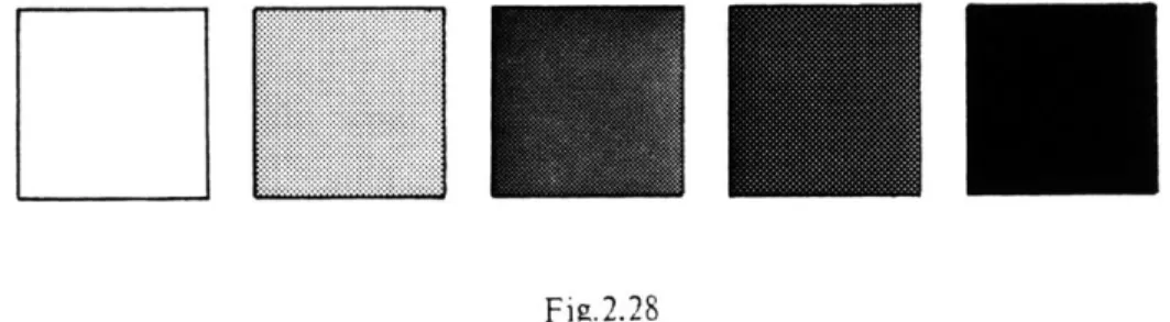
2.8 In natural denotation we can define qualities such as white (w), light- gray (1), gray (g), dark-gray (d) and black (b). All one-element qualitative structures defined

by these five qualities are shown in Fig.2.28. We know that all two-element qualitative

Fig. 2. 28

structures are unlimited and of one dimension. With a two-element generating set and

five given qualities

it

is possible to define ten homomorphic qualitative structures in

natural denotation (Fig.2.29). With a three-element generating set and five given

Fig.2.29

qualities it is possible to define ten homomorphic qualitative structures in natural

denotation (Fig.2.30). All these qualitative structures are limited two-dimension, with

two limits of the first order. In natural denotation it is not possible to define an

unlimited two-dimension qualitative structure, since in this denotation there is always

KI...l.

LI

D

DLI

D...

Lj

D

Fig.2.30

one lightest quality and one darkest quality as two limits of the structure. With a four-element generating set and five given qualities it is possible to define four homomorphic qualitative structures in natural denotation (Fig.2.31). And finally, with a

DLI

DIII

DLII...

LIII LIIIII

Fig.2.31

five-element generating set and five given qualities it is possible to define only one qualitative structure (Fig.2.32). This is also a limited two-dimension qualitative .structure since in natural denotation we can define only these neighborhood relations: w*1, l*g,

g*d, d*b. One can come to the conclusion that in natural denotation it is possible to

define only limited two-dimenson spatial structures (for n>2) with two limits of the first order represented by the lightest and darkest qualities. The lightest quality in the structure has one neighbor, which is the next lightest quality in the structure. The

D

D

Fig.2.32

lighter and one darker. We can extend the number of qualities in order to get a quality structure with a greater number of elements. We can define, for example, a new quality dark-white which is darker than white and lighter than light-gray. However, with this extension we can arrive again at a limited two-dimension qualitative structure since the new quality element (dark-white) has two neighbors: white and light-gray.

2.9 Let the two two-element qualitative structures be defined as shown in Fig.2.33. A qualitative structure, Sa, is defined by two qualities: black and white. We can

a Fig.2.33 b

assume that these two qualities relate one toward another as positive toward negative. the negative of white is black and negative of black is white. A qualitative structure,

Sb, is defined also by two qualities: light-gray and dark-gray. We can assume that

these two qualities also relate one toward another as positive toward negative. The negative of light-gray is dark-gray and vice versa. Two qualities which relate one toward another, as positive toward negative are complementary qualities. White is the complement of black (w=Ab), light-gray is the complement of dark-gray (l=Ad). A

48

quality is only and always gray (g=^g). A structure with an odd number of elements containing a neutral quality, with each quality having its complement, is a complete qualitative structure. The three-element qualitative structure shown in Fig.2.34a is complete since it contains a neutral quality (g) and two other qualities which are complementary (w=Ab). A structure with an even number of elements, each with its

complement, is a complete qualitative structure. The four-element qualitative structure

a

b

Fig.2.34

shown in Fig.2.34b is complete since white is the complement of black and light-gray is the complement of dark-gray (w=Ab, l=Ad). A complete five-element qualitative

structure can be defined by white, light- gray, gray, dark-gray and black qualities. In this structure (Fig.2.35a) white is the complement of black (w=Ab), light-gray is the

Fig.2.35 b

complement of dark-gray (l=Ad), and gray is the neutral quality (g=Ag). This complete qualitative structure is a limited two-dimension structure with two limits (white and black), defined by the following neighborhood relations: w*l, l*g, g*d, d*b. With the very same generating set and qualities we can define another limited two-dimension qualitative structure as shown in Fig.2.35b. In these two homomorphic structures, corresponding elements contain complementary qualities. The neutral quality gray is self-complementary. Two homomorphic qualitative structures are complementary if the corresponding elements contain complementary qualities. Examples of two-element complementary qualitative structures are shown in Fig.2.36. All three-element

D

Fig.2.36

r.

El

Dr

Fig.2.37

complementary qualitative structures should have one neutral quality element (gray) as shown in Fig.2.37. Examples of four and five-element complementary qualitative

structures are shown in Fig.2.38.

LTl

Fig.2.38

2.10 Let a three-element generating set be defined as shown in Fig.2.39. With this set we can define the three-element qualitative structure (w*g, g*b) shown in Fig.2.40a.

By definition, this structure contains three different qualities: white, gray and black.

50

shown in Fig.2.40b? This is a three-element structure defined by two qualities (white

and black). Therefore, there is only one neighborhood relation between qualities in

Fig.2.39

this structure (w*b), since the neighborhood relation between equal qualities is not

defined. Two elements in this structure contain the same quality (black). However, by

definition, in the qualitative structure there are no two elements with equal qualities.

One can come to the conclusion that this structure doesn' t correspond to the

a b

Fig.2.40

qualitative structure definition. Let some structure be defined with an n-element

generating set and q different qualities.

If n=q then this structure is a regular

qualitative structure as defined before. However, if n>q the structure must contain at

FWE

0H

ll

reduced qualitative structures with two qualities (q=2) and a different number of

DLII....

DLII.

....

D

EL

Fig.2.42

elements (n>2) are presented in Fig.2.41. A special type of reduced qualitative

structure can be defined as q=1 and n>1 (Fig.2.42). All these qualitative structures are one-quality structures, and the neighborhood relations between elements within the structures are not defined.

2.11 All reduced qualitative structures defined by the very same generating set are homogeneous (Fig.2.43). The difference between the number of elements and the number of qualities (n-q) of a reduced qualitative structure defines its degree of

D]

D

D

Fig.2.43

reduction (dr). For the regular qualitative structure, dr=O. Examples of qualitative structures with n=4 and q=1,2,3,4 are presented in Fig.2.44. The structure dr=O is a

MED

DD LIDN

Fig.2.44

one-quality structure with no neighborhood relations. The structure dr=2 is a two-quality structure with only one neighborhood relation (w*b). The structure d=1 is a three-quality structure with two neighborhood relations in natural presentation (w*l,

1*b). The last example, dr=O, is a regular qualitative structure with three neighborhood

relations in natural presentation (w*l, l*d, d*b). With one quality (q=1) we can define

WEN

DL]DI

Fig.2.45

only one qualitative structure without considering a number of elements, n. However, for the two-quality structure shown above (dr=2), for example, there are three possible reduced qualitative structures (Fig.2.45).

2.12 Two reduced qualitative structures (nl,ql) and (n2,q2) are isomorphic if they have nl=n2, ql=q2, and equal neighborhood relations (Fig.2.46). These three structures

Fig. 2.46

are isomorphic since nl=n2=n3=3 and ql=q2=q3=2, and the neighborhood relation between qualities is w*b for all three structures. Both homogeneous and isomorphic

Fig.2.47

(Fig.2.47). Two homomorphic reduced qualitative structures are complementary if all

corresponding elements contain complementary qualities (Fig.2.48). It will be important

Fig.2.48

to define a set whose elements are complementary reduced qualitative structures. Two

complementary one-quality reduced structures define a binary set (B-set). As we can

Fig.2.49

see in Fig.2.49, for example, a B-set can be defined by white and black or by

light-gray and dark-gray qualities. However, in further explication a B-set will be

defined only by white and black qualities as shown in Fig.2.50.

NINEl

E

CHAPTER III

STATE OF SPACE

3.1 Let a two-element generating set be S = (p,q) as shown in Fig.3.1a. With this

generating set, we know, it is possible to define both spatial and qualitative structures (Fig.3.1b). If the elements of qualitative structures occupy the positions of corresponding

pq

J

ILE

a

Fig.3.1 b

I1

Fig.3. 2

elements in a spatial structure we have a new type of structure. The unity of a spatial structure and qualitative structure defined by the same generating set determines

a state of space. With the spatial and qualitative structures shown in Fig.3.1b it is possible to define only one state of space. However, with the other two-element structures shown in Fig.3.3a we can define two states of space (Fig.3.3b). Both spatial

a

Fig.3.3

b

and qualitative structures defined by the very same generating set are corresponding structures. Structures shown in Fig.3.1a are corresponding, as well as the structures shown in Fig.3.3a.

3.2 The three-element

state of space (Fig.3.4b).

WEZ

_a

Fig.3.5a, we can define two three-element corresponding set

corresponding set shown in Fig.3.4a can define only one With another three-element corresponding set, shown in

b

Fig.3.4

states of space (Fig.3.6b). And finally, with the shown in Fig.3.6a we can define six different states of

LI~

I I

a Fig.3.5 b

space (Fig.3.6b). The number of different states of space defined by the same corresponding set is the potentiality of the corresponding set. The corresponding set

a

K I

D~

I

b

I

Fig.3.6

3.3 Two different states of space defined by the same corresponding set are shown

in Fig.3.7. The spatial and qualitative structures of a corresponding set both contain four elements and are limited and two-dimension. The qualitative structure is defined in natural presentation (w*l, l*d, d*b). We know that in qualitative structures the

L

..

1I..

b Fig.3.7

spatial neighborhood relations between elements is not defined. However, in the state of space all elements of a qualitative structure have spatial neighborhood relations defined by the corresponding spatial structure. In the first state of space shown in

Fig.3.7b, the spatial neighborhood relations between qualities are: w*1, 1*d, d*b. We

can see that they are equal to the given neighborhood relations between qualities defined by the corresponding qualitative structure. However, in another state white is the neighbor of black, and light-gray and dark-gray are not spatial neighbors. The spatial neighborhood relations between qualities in this state are: l*w, w*b, b*d. It is

58

obvious that these relations are not equal to the neighborhood relations defined by a given qualiatative structure. Such a state of space in which spatial neighborhood relations between qualities are equal to the neighborhood relations between qualities in a qualitative structure we will designate the natural state. We can now conclude that the first state of space shown in Fig.3.7b is natural and the other one is not. Examples of some natural states of space are shown in Fig.3.8. The corresponding qualitative structures are defined in a natural presentation.

Fig.3.8

3.4 Let two different states of space be defined as shown in Fig.3.9. The spatial neighborhood relations between qualities in these two states are: a. w*g, g*b; and b. w*g. g*b. We can see that these spatial neighborhood relations are equal. Two states

a _b

Fig. 3.9

of space are isomorphic if they have equal spatial neighborhood relations between qualities. Examples of some isomorphic states of space are shown in Fig.3.10. The spatial neighborhood relations between qualities for these states of space are:

a. w*g. w*b, g*b; c. l*w, w*d, d*b; b. g*w, w*b; d. w*l, l*d, d*b;

m

b

Fig.3.10

3.5 Let two different states of space be defined as shown in Fig.3.11. These two states are homogeneous since they are defined by the very same corresponding set. In addition, these two states are isomorphic because of the equal spatial neighborhood

Fig.3.11

relations between qualities: w*g, g*b. Both isomorphic and homogeneous states of space are homomorphic. Examples of some homomorphic states are shown in Fig.3.12.

Fig.3.12

Two states of space are equal if equal qualities occupy equal positions. Given the current definition of the corresponding set, equal states of space are also homomorphic (Fig.3.13).

Fig.3.13

3.6 With the corresponding set defined by a regular qualitative structure we can

generate only states in which different qualities occupy different positions (Fig.3.14a). In this kind of state there are no two different positions with equal qualities.

a b

Fig.3.14

Therefore, it is not possible to define, for example, a state of space as shown in Fig.3.14b. In order to generate such a state we should define the corresponding set by a reduced qualitative structure. A corresponding set defined by a reduced qualitative structure we will designate the reduced corresponding set or RC-set. The RC-set

which can define the state of space shown above (Fig.3.14b) is presented in Fig.3.15a. With this RC-set it is also possible to define some other states of space, as shown in

b Fig.3.15

Fig.3.15b. However, with another corresponding set, shown in Fig.3.16a, we can define such a state (Fig.3.16b) which is equal to the last state shown in the previous figure.

b

Fig.3.16

These two structures are equal since equal qualities occupy equal positions. Two equal states are identical if they are homomorphic (Fig.3.17).

3.7 Such a corresponding set defined by one spatial structure (n>1) and one-quality

qualitative structure can generate only one state of space (Fig.3.18). It is important to

Fig.3.18

define such a corresponding set which can generate both one-quality and two-quality states of space, as shown in Fig.3.19. All these states can be generated by the

corresponding set of two-element spatial structure and the B-set shown in Fig.3.20. A

Fig.3.19

Fig.3.20

corresponding set defined by one spatial structure and a B-set we will designate the B-corresponding set or BC-set. With the BC-set shown in Fig.3.21a we can generate

DD

H..IME

a

b Fig.3.21

states of space shown in Fig.3.21b. However, these are only a few examples of the 81 different states we can generate with the BC-set shown in Fig.3.21a. With another

Fig.3.22 a

BC-set shown in Fig.3.22a we can generate only 16 different states (Fig.3.22b). All

states defined by the BC-set are the B-states (binary states).

]

F-i-Fig.3.32b

3.8 We can now define some new terms within

spatial characteristics. Usually these new terms will Fig.3.23

the state of space regarding its be denoted by a black quality.

E:1

MR 01

IN

(Fig.3.24). The two elements with the same quality (black) shown in Fig.3.25 are not a

Fig.3.24

Fig.3.25

couple since both black elements are surrounded by white elements. Therefore these elements are two isolated points.

3.8.2 Three and more connected neighboring elements with the same quality (black),

with at least one element with two neighbors, and no elements with three or more neighbors is the line. Examples of a three-point line, defined in different

configurations, are presented in Fig.3.26. A line is open if it contains two points with

one neighbor (two ends) as shown in Fig.3.26a. A line is closed if all points of a line have two neighbors. A minimal (three-point) closed line is a triplet (Fig.3.26b).

OEHi

b

Fig.3.26

3.8.3 With four connected points we can define both open and closed lines. Some

examples of four-point open and closed lines are shown in Fig.3.27. All four-point open lines are spatially isomorphic, as are all four-point closed lines, regardless of the differences between the structures in which they are defined. Two open (closed) lines with an equal number of points are isomorphic. Two isomorphic lines defined in equal

a

b

Fig.3.27

spatial structures are homomorphic (Fig.3.28). Therefore, the five-point open lines shown in Fig.3.28a are homomorphic. The five-point open lines shown in Fig.3.28b are homomorphic too. In addition, all these five-point open lines are isomorphic.

FK]

b

Fig.3.28

3.8.4 Between two isolated points in the structure we can define many different lines, as shown

elements (ends),

in Fig.3.29. The number of line points, including the terminating determine the length of the line. The minimum line that can be

a b C d e

Fig.3.29

charted between two points is the distance. Therefore, the length of the line shown in Fig.3.29a, for example, is 1=5 and the distance between the line ends is d=3.

According to this, the length of the couple is 1=2 but the distance between the points

a _b

Fig.3.30

of a couple is d=O. Also, the length of the triplet is 1=2 but the distance between

any two points of the triplet is d=O. Another interesting example is presented in Fig.3.30. The distance between points A and B is two (d=2) and there is only one

possible distance between these two points. However, for the distance between points

A and C (d=3) there are four different possibilities, as shown in Fig.3.30b. Let an

isolated point be defined as shown in Fig.3.31a, and let all the points with the same distance (d=2) from the given point be defined as shown in Fig.31b. These are all possible points with the distance two from the given point. in this structure. We can easily determine that all these equidistant points are isolated. However, even when they

a b

Fig.3.31

are all isolated points, they divide the entire structure into two areas: exterior and interior. The interior is the area where the given point is located. It is not possible to define any connected line in which one end belongs to the interior and another belongs to the exterior. These are some interesting spatial characteristics for the structures shown above. Each spatial structure represents a specific universe of positions and neighborhood relations with its own topological characteristics. What is

possible in one spatial structure, may not be possible in another. In a limited

two-dimension structure, for example, it is not possible to define a closed line. It is also not possible to define a line whose length is greater than the number of elements of the structure (<n).

ab

Fig.3.32

3.8.5 _{Two lines with one common point define an intersection (Fig.3.32). An}