HAL Id: hal-00296962
https://hal.archives-ouvertes.fr/hal-00296962
Submitted on 26 Sep 2006
HAL is a multi-disciplinary open access
archive for the deposit and dissemination of
sci-entific research documents, whether they are
pub-lished or not. The documents may come from
teaching and research institutions in France or
abroad, or from public or private research centers.
L’archive ouverte pluridisciplinaire HAL, est
destinée au dépôt et à la diffusion de documents
scientifiques de niveau recherche, publiés ou non,
émanant des établissements d’enseignement et de
recherche français ou étrangers, des laboratoires
publics ou privés.
Storage cascade vs. MODFLOW for the modelling of
groundwater flow in the context of the calibration of a
hydrological model in the Ammer catchment
V. Rojanschi, J. Wolf, R. Barthel
To cite this version:
V. Rojanschi, J. Wolf, R. Barthel. Storage cascade vs. MODFLOW for the modelling of groundwater
flow in the context of the calibration of a hydrological model in the Ammer catchment. Advances in
Geosciences, European Geosciences Union, 2006, 9, pp.101-108. �hal-00296962�
www.adv-geosci.net/9/101/2006/ © Author(s) 2006. This work is licensed under a Creative Commons License.
Advances in
Geosciences
Storage cascade vs. MODFLOW for the modelling of groundwater
flow in the context of the calibration of a hydrological model in the
Ammer catchment
V. Rojanschi, J. Wolf, and R. Barthel
Institute for Hydraulic Engineering, University of Stuttgart, Germany
Received: 23 January 2006 – Revised: 22 May 2006 – Accepted: 3 July 2006 – Published: 26 September 2006
Abstract. Hydrological models are the decisive tools to evaluate the effect of global change upon the water cycle. But the applied hydrological models have to be a trade-off between their degree of complexity and manageable struc-tures and data requirements. This paper compares the advan-tages and disadvanadvan-tages of integrating a spatially-distributed process-based groundwater flow model in the context of the calibration of a catchment runoff concentration model. The multi-objective optimisation and the GLUE method are used to analyse the performance and the parameter identifiability of both model structures.
1 Introduction
Different motivations and goals can be the reason for build-ing a hydrological model. They play also an essential role on the choice of the modelling structure and of the modelling strategy. One main dilemma concerns the degree of complex-ity to be chosen, or the degree of conceptualcomplex-ity of the model. It is widely accepted that a simple and efficient conceptual structure with very few parameters is the logical choice if the task to be solved is the correct reproduction of river dis-charge time series, for example for flood protection studies or for the evaluation of the hydropower potential of a certain river reach. For other tasks the answer to the above dilemma is less clear. Especially in the context of Global Change, in which a comprehensive description of the effects of possible future climate and socio-economical changes on the water cycle is required, the determination of the appropriate model structure is a challenging research topic.
The present paper reports on a study about the advan-tages and disadvanadvan-tages of including a distributed physically-based groundwater flow model into a hydrological catchment
Correspondence to: V. Rojanschi
(vlad.rojanschi@iws.uni-stuttgart.de)
model. The groundwater flow model uses the Boussinesq equation to compute the groundwater level and groundwa-ter flow rates for each cell of a given grid. It is a signifi-cant qualitative and quantitative improvement to the storage-based conceptual models (e.g. Singh, 1995), since it offers a better representation of the physical processes and it yields more computed variables. On the other hand it is not ob-vious whether the inclusion of the distributed groundwater flow model would improve the performance of the catch-ment model or the identifiability of its parameters. Moreover it is questioned whether the results of the sectoral calibra-tion and validacalibra-tion of the groundwater flow model with mea-sured groundwater level time series can be directly applied on the hydrological model, which concentrates more on dis-charge time series. An additional issue tackled in this study is the comparison between two state-of-the-art methodolo-gies in hydrological modelling: multi-objective optimisation and GLUE. Case study for this work is the Ammer catch-ment, located in the Southern Bavarian alpine and pre-alpine zone (Fig. 1).
2 Modelling concept and strategy
The main idea behind this study is to build and parameterise the two models (for groundwa-ter flow and for catchment hydrology) independently from each other so that they both fulfill the standard sectoral goals set for the verification of such models. Afterwards the groundwater flow model is in-cluded in the hydrological catchment model and the resulting changes in the performance of the catchment model are eval-uated.
The structure of the used hydrological catchment model is presented in Fig. 2 (see also Ro-janschi et al., 2005). The runoff formation is computed by the grid based SVAT-model PROMET (Mauser, 1989). PROMET includes modules for the radiation balance, evapotranspiration, snow accumulation
102 V. Rojanschi et al.: Storage cascade vs. MODFLOW
Fig. 1. The Ammer catchment in Southern Bavaria, Germany.
and melting, water consumption by vegetation and soil water balance. For the last module a development of the Richard’s equation (Eagleson, 1978) is applied on a two meter thick soil layer to compute a surface runoff and a percolation rate out of the soil zone. For the purpose of this study the soil per-colation of the PROMET model, computed and made avail-able by Prof. R. Ludwig, Kiel University, were used subse-quently for the simulations with both model versions. The runoff concentration is represented by means of four concep-tual modules, for the implementation of which linear storage cascades (Nash, 1959) were used. One additional storage cascade for every river stretch routes the total river discharge from one gauge to the next one (Unit E5). The integration of the distributed groundwater flow model is done by replacing the storage cascade (hydrological model case 1) in Unit E4 with a MODFLOW (McDonald and Harbough, 2000) model (case 2).
For the calibration and the validation of hydrological model and the quantification of the parameter indentifiabil-ity, several methods coexist without having one that is clearly better in all aspects. Two of them were selected for the present study: the multi-objective optimisation (Gupta et al., 1998) and the generalised sensitivity based GLUE technique (Beven and Binley, 1992).
The idea behind the multi-objective optimisation is that several quite different solutions can have the same value of a particular objective function when they are compared to mea-sured data. As a consequence one should use multiple ob-jective functions in the optimisation process to better charac-terise a solution (also a set of parameter values). The solution of such an approach is the Pareto set: the group of solutions, optimising as a group the chosen objective functions.
The GLUE-Analysis rejects the concept of an optimal rameter set altogether. After generating a large sample of pa-rameter sets, one differentiates between the sets which lead to good model results (the so called behavioural sets) from the ones with poor results (non-behaviour). The statistical analysis of the behavioural values is then a measure for the sensitivity of the parameters and for the uncertainty in the modelling process.
The multi-objective optimisation consists in computing multiple solutions optimising as a group the chosen math-ematical objective functions. A combination of the global Simulated-Annealing and the local Downhill-Simplex algo-rithms (Press et al., 1992) and a linear weighting system were used for the determination of the group of solutions, termed Pareto set. Six functions were chosen for the analysis with the aim of quantifying the quality of the model results for the
Soil Water Model Infiltration above mountain slopes Infiltration above valley aquifers Surface Runoff Surface Runoff Baseflow Interflow Finite-Difference Groundwater Flow Model
s measured Discharge River Model Unit 1 Unit 3 Unit 2 Unit 4 Soil Water Model
Infiltration above mountain slopes Infiltration above valley aquifers Surface Runoff Surface Runoff Baseflow Interflow Finite-Difference Groundwater Flow Model
s measured Discharge River Model Unit 1 Unit 3 Unit 2 Unit 4
Fig. 2. The structure of the hydrological model in the Ammer catchment.
different significant parts of the discharge hydrographs (the entire time series, the ascending and the descending parts, see also Freer, 2003): the Sutcliffe efficiency (N S), Nash-Sutcliffe efficiencies computed for the increasing and the de-creasing part of the hydrographs (N Sdr, N Sndr), SAE=1−S,
where S is the sum of the absolute differences between Qmes
and Qsimnormalised by the sum of Qmes, the Nash-Sutcliffe
efficiency computed between Qmes and Qsim after
apply-ing a Box-Cox transformation (N St r – the transformation
changes the discharge values such that they become approxi-matively normally distributed, thus avoiding the overweight-ing of the high values, Box and Cox, 1964) and the average linear correlation Kgr between the measured and the
com-puted groundwater level timeseries. The last function Kgr
could be used only in the version with the integrated MOD-FLOW model.
The same objective functions were used as likelihood mea-sures for the GLUE analysis to-gether with a direct-sampling generation of parameter sets. To differentiate between be-havioural and non-bebe-havioural sets the value of each objec-tive function was compared to the corresponding local op-tima computed during the multi-objective optimisation. If for a parameter set the difference between the two values was smaller than a chosen limit (0.1) for all the considered objec-tive functions and for both the calibration and the validation time series, the set was classified as behavioural.
3 Finite-difference groundwater flow model in the Am-mer catchment
The Ammer catchment with a total surface of 709 km2 is located in the transition zone between the Calcareous Alps and their foreland (molasse). In this mountainous area the
groundwater flow is part of the short term hydrological cycle and takes place almost only in the alluvial aquifers. All other geological layers have negligible influence. The rocks of the Calcerous Alps show only a minor degree of karstification in this area (Doben, 1976). Therefore a one-layered groundwa-ter model of the alluvial aquifers was built (the extent of the aquifer is added in Fig. 1). The aquifer was assumed to be un-confined, but for reasons of the model’s stability a minimum saturated thickness of 5 meters was chosen in order to avoid dry cells. The discretisation of the model is 1000 m×1000 m in order to keep calculation times of the overall model cali-bration and the storage demand of the output data manage-able. Since the geometry of the alluvial aquifer is very com-plicated and the extent is very small for a square kilometre discretisation, a new approach had to be developed to imple-ment the aquifer geometry into a numerical model. This ap-proach expands the concept of hydrological drainage analy-sis (Fairfield and Leymarie, 1991) to the groundwater runoff. The geometry of the alluvial aquifers is adjusted in a way that groundwater runoff can be accumulated to the catchments gauge and guarantees continues groundwater flow (Wolf et al., 2004).
The recharge in the Ammer catchment that percolates from the soil outside the alluvial aquifers is transferred to the groundwater model by using the calculated flow direction of the drainage analysis model TOPAZ (Garbrecht and Martz, 1995). Losses due to carstification are less important. But the subsurface groundwater flow to the neighbouring Loisach valley (this flows outcrops in the Maulenbach spring with a nearly constant outflow of 1 m3/s, see Fig. 1), has to be taken into account by the groundwater model.
First a stationary model was built and analysed. During calibration the model’s parameters were estimated with an
104 V. Rojanschi et al.: Storage cascade vs. MODFLOW 547 548 549 550 551 552 0 200 400 600 800 1000 OBS1:i=11,j=23 MAE=0.91,CORR=0.51 549 550 551 552 553 554 0 200 400 600 800 1000 OBS2:i=12,j=23 MAE=0.49,CORR=0.47 549 550 551 552 553 554 0 200 400 600 800 1000 OBS3:i=12,j=23 MAE=0.37,CORR=0.46 552 553 554 555 556 557 0 200 400 600 800 1000 OBS4:i=13,j=23 MAE=1.20,CORR=0.28 552 553 554 555 556 557 0 200 400 600 800 1000 OBS5:i=13,j=23 MAE=0.38,CORR=0.37 602 603 604 605 606 607 0 200 400 600 800 1000 OBS6:i=20,j=26 MAE=0.31,CORR=0.75 611 612 613 614 615 616 0 200 400 600 800 1000 OBS8:i=23,j=27 MAE=0.36,CORR=0.76 640 644 648 652 656 660 0 200 400 600 800 1000 OBS9:i=29,j=25 MAE=4.69,CORR=0.54 860 870 880 890 900 910 0 200 400 600 800 1000 OBS10:i=44,j=15 MAE=9.25,CORR=0.55
Fig. 3. Computed (black line) vs. observed (gray line) groundwater levels (in masl) in nine observation wells in the Ammer catchment
(location see Fig. 1). The simulation period contained 1000 days from 01.01.95 to 26.09.1997.
trial and error approach based on 20 different zones. The allowed parameter values were bounded by measured data (mean values for permeability 1.15×10⁻³m/s and 0.16 for the storage yield). The result of this stationary model was then used as starting heads for the transient model runs, which were analysed and compared to observed data. For nine observation wells daily time series for the period from 1 January 1995 to 16 September 1997 (1000 days) were avail-able. The first 500 days were used for calibration, the second 500 days for validation.
The results are very satisfying for a coarse grid ground-water model: The mean average error is 1.95 m, the average correlation coefficient between computed and observed time series is 0.52 (Fig. 3).
4 Hydrological model: performance and parameter identifiability
The model structure in Fig. 2 and the methodology described in Sect. 2 were applied for the seven subcatchments delimited in the study area. For the purpose of this paper the presen-tation of the results is concentrated on the subcatchment up-stream of gauge Peissenberg, to which the ID 3 was given here (Fig. 1).
Table 1 presents the optimal values for all used objective functions of the multi objective optimisation during the cali-bration (1 November 1993–1 January 2000) and validation (1 November 1990–31 October 1993) periods and for the two model versions (Case 1 with a storage cascade for the groundwater module and Case 2 with the integrated MOD-FLOW model). For Case 1 the different indicators of the model performance are all above 0.83 indicating that the model reproduces very well all elements of the measured discharge time series. Figure 4 confirms this observation,
Table 1. The optimal values for the applied objective functions of the multi objective function in subcatchment 3 (gauge Peissenberg). Subcatchment 3 NS NSdr NSndr SAE NStr KGr NS NSdr NSndr SAE NStr KGr Case 1 0.92 0.89 0.83 0.85 0.89 0.90 0.86 0.89 0.85 0.89 Case 2 (MODFLOW) 0.88 0.85 0.81 0.83 0.85 0.64 0.87 0.83 0.89 0.84 0.85 0.62 Calibration Validation
Fig. 4. Computed (grey lines represents the different Pareto sets) vs observed (black line) discharge time series for the hydrological year
1998 in subcatchment 3 for both model structures.
although the model shows weaknesses when it comes to modelling the winter events (which might be connected to the special difficulty of correctly estimating winter precipita-tion in alpine regions).
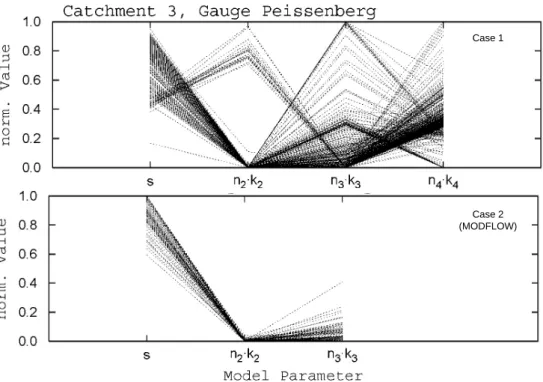
Estimations of the uncertainty in the determination of the parameter values are given in Fig. 5 (multi-objective opti-misation) and Fig. 6 (GLUE). Beside the separation param-eter s be-tween vertical and horizontal flow component in the percolation zone the parameters of the storage cascades are analysed for the percolation zone (Unit E2 and E3) and groundwater (Unit E4). For a storage cascade the product of its two parameters, n and k, which is the time interval with which the centre of gravity of the input signal is shifted for-ward into the output signal, was chosen for the analysis. n and k can compensate each other in a relatively large amount so an individual calibration is not meaningful, if an uncer-tainty analysis is planed.
For Case 1 the results of the multi-objective optimisation show that s is the only parameter, whose values are clearly concentrated in one specific region of the interval. For n3·k3 and n4·k4 optimal values were found throughout the whole
interval and for n2·k2 they are grouped at the two interval ex-tremities. However, the possibility to visually identify “con-centration” zones in which the density of optimal values is clearly larger than elsewhere could entitle a modeller to qual-ify the results as only moderately uncertain.
The GLUE analysis in Fig. 6 contradicts strongly this de-scription. While s stays well determined (less clear though than in Fig. 5) the other three appear almost perfectly unde-termined suggesting a strong over-parameterisation and in-teractions between the model parameters. The difference be-tween the two sets of results, which were obtained for the same model with the same data and the same objective func-tions, are a very good indications for the difference between the two modelling approaches. GLUE has less strict accep-tance criteria than the multi-objective optimisation and this leads also to a more negative estimation of the parameter identifiability.
For the integration of the MODFLOW model in Case 2 the parameters of the groundwater flow model, which were determined during the stand-alone calibration (Sect. 3), were kept fixed for both the multi-objective and the GLUE
106 V. Rojanschi et al.: Storage cascade vs. MODFLOW
Case 1
Case 2 (MODFLOW)
Fig. 5. Parameter uncertainty of the multi-objective optimisation approach for subcatchment 3. The calibration intervals for all parameters
were normalised to [0,1]. Each plotted line stands for one point in the multi-objective solution. The spreading of the values inside the solution for one specific parameter quantifies the uncertainty in determining that parameter.
Case 1
Case 2 (MODFLOW)
Fig. 6. Parameter uncertainty of the GLUE method for subcatchment 3. Each point represents a generated parameter set which lead to model
results characterised by a performance values shown on the y-axis. Very different parameter values leading to the same quality of the results is a sign of a high non-identifiability of the parameters.
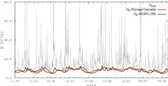
Fig. 7. Comparison of the groundwater flow from the MODFLOW model (Case 2) and out of the storage cascade (Case 1) for the whole
Ammer catchment.
analysis, which lead to a reduction of the number of varying parameters. The implications for the model performance can be observed in Table 1 and Fig. 4. Although the values for the objective functions can be still qualified as very good, a slight deterioration is to be noticed, proving that the param-eters from the stand-alone calibration of one model part are not the optimal values for the hydrological model as a whole. An interesting comparison is however the one between the groundwater flow out of the linear storage cascade and out of the MODFLOW model (Fig. 7, the 50% quantiles of the GLUE solutions are plotted). Their performance, measured to the total river discharge, was almost the same with a light advantage for the cascade. The fraction of the groundwater flow to the total discharge was also almost identical (61% in Case 1 and 63% in Case 2) As no direct measurements for the groundwater exfiltration are available the evaluation must remain qualitative and therefore subject to disputable interpretation. The authors of this paper think, however, that the dynamics of the MODFLOW curve is much more real-istic than for the storage cascade. The simple two param-eter function of the cascade is by far not able to reproduce the complexity of a physically based flow model. Addition-ally, a systematic shift forward with about two months can be noticed on the cascade curve. During the optimisation the groundwater flow curve is damped, which can be achieved in linear storage cascade only by simultaneous increase of the shifting interval. As a result the dynamics of the groundwater flow is false until large time scales, this having implications on the applicability of such models for questions focusing on groundwater resources management.
Regarding the uncertainty in the parameter determination (Figs. 5 and 6) the differences between the two applied meth-ods are noticeable also for Case 2. While the reduction of
free parameters lead to a clear improvement during the multi-objective optimisation the GLUE distributions stay almost equally uniform over the whole interval, a sign that adding the groundwater level to the river discharge for calibrating parameters of hydrological model is a step in the right direc-tion, but not the solution to the problem of parameter uncer-tainty.
5 Conclusions
Two hydrological models were applied for the Ammer catch-ment located in Southern Bavaria. A conceptual hydrologi-cal model and a physihydrologi-cally-based groundwater flow model. The groundwater flow model was parameterised as a stand-alone model and then integrated in the conceptual hydrologi-cal structure. The performance of the latter one in its two ver-sions, with a linear storage cascade or with the MODFLOW model for the groundwater module, was then analysed from the point of view of model performance and of the parameter identifiability.
Both model versions were able to reproduce very well the river discharge time series (Fig. 3). Reducing the number of degrees of freedom by integrating the MODFLOW model with fixed parameter values lead to slight deterioration, com-pensated, however, by the fact that the model output was sig-nificantly increased with calculated values for groundwater levels and groundwater flow field. The main improvement was of qualitative nature: the dynamics of baseflow curve was judged to be much more realistic when the MODFLOW model was used, so that the corresponding model version is more appropriate for studies in which the evaluation of groundwater resources is needed.
108 V. Rojanschi et al.: Storage cascade vs. MODFLOW The interpretation of the results for the parameter
inter-pretability is less clear, as the two used methods lead to different conclusions. According to the multi-objective op-timisation reducing the number of free parameters and ad-ditionally conditioning the model to the groundwater lev-els did have a significant reduction of the parameter uncer-tainty. This statement was contradicted by the GLUE results which showed for both model versions almost perfectly uni-dentifiable parameters.
The less strict acceptance criteria in GLUE leads system-atically to a larger estimated uncertainty. When this issue is not of concern, it is obvious that the model output after a multi-objective optimisation fits mathematically better the measured data. When it comes to giving a physical interpretation to the calibrated parameter values, GLUE’s conservatory view seems more appropriate than the over-confident multi-objective optimisation.
Edited by: R. Barthel, J. G¨otzinger, G. Hartmann, J. Jagelke, V. Rojanschi, and J. Wolf
Reviewed by: anonymous referees
References
Beven, K. J. and Binley, A.: The future of distributed models: model calibration and uncertainty prediction, Hydrol. Processes, 6, 279–298, 1992.
Box, G. E. P. and Cox, D. R.: An analysis of transformation, J. Roy. Stat. Soc., B26, 211–252, 1964.
Doben, K.: Erl¨auterungen zur Geologischen Karte von Bayern 1:25 000, Blatt Nr. 8433 Eschenlohe, Bayerisches Geologisches Landesamt, M¨unchen, 1976.
Eagleson, P. S.: Climate, Soil and Vegetation, 3, A simplified model of Soil Moisture Movement in the Liquid Phase, Water Resour. Res., 14, 5, 722–730, 1978.
Fairfield, J. and Leymarie, P.: Drainage Networks from Grid Digital Elevation Models, Water Resour. Res., 27, 3, 709–717, 1991.
Freer, J., Beven, K., and Peters, N.: Multivariate Seasonal Period Model Rejection within the Generalised Likelihood Uncertainty Estimation Procedure, Water Sci. Appl., 6, 9–29, 2003. Harbaugh, A. W., Banta, E. R., Hill, M. C., and McDonald, M.
G.: MODFLOW-2000, The U.S. Geological Survey Modular Ground-Water Model – User Guide to Modularization Concepts and the Ground-Water Flow Process, U.S. Geological Survey, Open-File Report 00-92, 2000.
Garbrecht, J. and Martz, L. W.: TOPAZ: An automated digital landscape analysis tool for topographic evaluation, drainage identification, watershed segmentation and subcatch-ment parametrization – TOPAZ User Manual, USDA-ARS Pub-lication No. NAWQL 95-3, USDA-ARS, Durant, Oklahoma, 1995.
Gupta, V. H., Sorooshian, S., and Yapo, P. O.: Towards improved calibration of hydrologic models: Multiple and noncommensu-rable measures of information, Water Resour. Res., 34, 4, 751– 763, 1998.
Mauser, W.: Die Verwendung hochaufl¨osender Satellitendaten in einem Geographischen Informationssystem zur Model-lierung von Fl¨achenverdunstung und Bodenfeuchte, Dissertation, Albert-Ludwigs-Universit¨at Freiburg i. Br., 1989.
Nash, J. E.: Systematic determination of unit hydrographs parame-ters, J. Geophys. Res., 64, 111–115, 1959.
Press, W. H., Teukolsky, S. A., Vetterling, W. T., and Flannery, B. P.: Numerical Recipes in Fortran 77, Cambridge University Press, New York, USA, 1992.
Rojanschi, V., Wolf, J., Barthel, R., and Braun, J.: Using multi-objective optimisation to integrate alpine regions in groundwater flow models, Adv. Geosci., 5, 19–23, 2005,
http://www.adv-geosci.net/5/19/2005/.
Singh, V. P.: Computer Models of Watershed Hydrology, Water Re-sour. Publ., Highlands Ranch, Colorado, USA, 1995.
Wolf, J., Rojanschi, V., Barthel, R., and Braun, J.: Modellierung der Grundwasserstr¨omung auf der Mesoskala in geologisch und geomorphologisch komplexen Einzugsgebieten, in: 7. Workshop zur großskaligen Modellierung, p. 155–162, Kassel University Press, 2004.