A DIGITAL SPECTRAL ANALYSIS TECHNIQUE AND ITS APPLICATION TO RADIO ASTRONOMY
by
SANDER WEINREB
B.S., Massachusetts Institute of Technology
SUBMITTED IN PARTIAL FULFILLMENT OF THE REQUIREMENTS FOR THE DEGREE OF
DOCTOR OF PHILOSOPHY
at the
MASSACHUSETTS INSTITUTE OF TECHNOLOGY
February, 1963
'1
Signature of AuthorDepartment of ElIctrical Engine7 ing, January 7, 1963
Certified by
Thesis Supervisor Accepted by I
A DIGITAL SPECTRAL ANALYSIS TECHNIQUE AND ITS APPLICATION TO RADIO ASTRONOMY
by
SANDER WEINREB
Submitted to the Department of Electrical Engineering on January 7, 1963 in partial fulfillment of the re-quirements for the degree of Doctor of Philosophy.
ABSTRACT
An efficient, digital technique for the measurement of the autocor-relation function and power spectrum of Gaussian random signals is described. As is quite well known, the power spectrum of a signal can be obtained by a Fourier transformation of its autocorrelation function. This paper presents an indirect method of computing the autocorrelation function of a signal having Gaussian statistics; this method greatly re-duces the amount of digital processing that is required.
The signal, x(t), is first "infinitely clipped"; that is, a signal, y(t), is produced, where y(t)= 1 when x(t) > 0 and y(t)= -1 when x(t) < 0. The normalized autocorrelation function, p (V), of the clipped signal is then calculated digitally. Since y(t) can be oded into one-bit samples, the autocorrelation processing (delay, storage, multiplication, and summa-tion) can be performed quite easily in real time by a special purpose digital machine - a one-bit digital correlator. The resulting py(-T) can then be corrected to give the normalized autocorrelation function, Px(),
of the original signal. The relation is due to Van Vleck and is simply p (r)
=
sin [- p (t)/2].The paper begins with a review of the measurement of power spec-tra through the autocorrelation function method. The one-bit technique of computing the autocorrelation function is then presented; in particular the-mean and variance of the resulting spectral estimate are investigated.
These results are then applied to the problem of the measurement of spectral lines in radio astronomy. A complete radio astronomy system is described. The advantages of the system are: 1) It is a multichannel system; that is, many points are determined on the spectrum during one time interval,- 2) Since digital techniques are used, the system is very accurate and highly versatile. The system that is described was built for the purpose of attempting to detect the galactic deuterium line. The last three chapters describe the results of tests of this system, the deuterium line attempt, and an attempt to measure Zeeman splitting of the 21 cm hydrogen line.
Thesis Supervisor: Jerome B. Wiesner Title: Institute Professor
iii
ACKNOWLEDGMENT
My first thanks must go to Dr. H. I. Ewen who, in 1957, aroused my interest in radio astronomy and suggested the deuterium-line search to me. Dr. Ewen also made a generous contribution to the initial financing
of this work.
Next, I would like to thank my supervisor, Prof. J. B. Wiesner, for encouraging me to undertake this research as a doctoral thesis, being ever so helpful in obtaining technical and financial support; and, by his interest and quality of leadership, being a constant source of inspiration for my work. It is fortunate for me that he was present at M. I. T. long enough to fulfill these first two functions and that his presence was not required for the third function.
Many people have been sources of encouragement and helpful tech-nical discussions concerning various aspects of the thesis. I would especially like to thank Dr. R. Price of Lincoln Laboratory, Profs. A. G. Bose and A. H. Barrett of M. I. T., Prof. A. E. Lilley of Harvard College Observatory, and Drs. F. D. Drake, D. S. Heeschen, and
T. K. Mennon of the National Radio Astronomy Observatory. I am thankful to the founders and staff of the National Radio
Astronomy Observatory for providing the excellent observing facilities and supporting help. My stay at Green Bank was one of the most pleasant and stimulating periods of my life.
The facilities of the M. I. T. Computation Center were used for part of this work. I appreciate the programming assistance provided by Mr. D. U. Wilde at M. I. T. and by Mr. R. Uphoff at Green Bank.
This work was supported in part by the National Science Foundation (grant G-13904) and in part by the U. S. Army Signal Corps, the Air Force Office of Scientific Research, and the Office of Naval Research.
iv TABLE OF CONTENTS Page CHAPTER 1. 1. 1 1. 2 1. 3 1.4 1. 5 1. 6 CHAPTER 2. 2. 1 2. 2 2. 3 INTRODUCTION Statistical Preliminaries
Definition of the Power Spectrum General Form of Estimates of the Power Spectrum
Comparison of Filter and Autocorrelation Methods of Spectral Analysis
Choice of the Spectral Measurement Technique
The One-Bit Autocorrelation Method of Spectral Analysis
THE AUTOCORRELATION METHOD OF MEASURING POWER SPECTRA
Introduction
Mean of the Spectral Estimate
2. 2-1 Relation of P*(f) to P(f)
2. 2-2 The Weighting Function, w(nAT) 2. 2-3 Some Useful Properties of P*(f) Covariances of Many-Bit Estimates of the Autocorrelation Function and Power Spectrum
2. 3-1 Definitions: Relation of the Spectral Covariance to the Autocorrelation Covariance 1 2
8
11 13 21 27 32 32 3636
39 4244
45
V
TABLE OF CONTENTS (Continued)
Page 2. 4 CHAPTER 3. 3. 1 3. 2 3. 3 3. 4 CHAPTER 4. 4. 1 4. 2
2. 3-2 Results of the Autocorrelation Covariance Calculation
2. 3-3 Results of the Spectral Covariance Calculation
Normalized, Many-Bit Estimates of the Spectrum and Autocorrelation Function
2. 4-1 Mean and Variance of the Normalized Autocorrelation Function
2. 4-2 Mean and Variance of the Normalized Spectral Estimate
THE ONE-BIT METHOD OF COMPUTING AUTOCORRELATION FUNCTIONS
Introduction
The Van Vleck Relation
Mean and Variance of the One-Bit Autocorre-lation Function Estimate
Mean and Variance of the One-Bit Power Spectrum Estimate
THE RADIO-ASTRONOMY SYSTEM The System Input-Output Equation Specification of Antenna Temperature 4.2-1 Correction of Effect of Receiver
Bandpass 4. 2-2 Measurement of T av
50
5255
57
60
60
64
66
71
76
76
80
84
vi
TABLE OF CONTENTS (Continued)
Page
4. 2.-3 Measurement of Tr (f+fo)
85
4.2-4 Summary
86
4. 3 The Switched Mode of Operation 87
4. 3-1 Motivation and Description 87 4. 3-2 The Antenna Temperature Equation 93
4. 4 System Sensitivity 94
CHAPTER 5. SYSTEM COMPONENTS 98
5. 1 Radio Frequency Portion of the System 98
5. 11 Front-End Switch and Noise Source 98
5. 1-2 Balance Requirements 101
5. 1-3 Shape of the Receiver Bandpass,
G(f+f ) 103
5. 1-4 Frequency Conversion and Filtering 105
5. 2 Clippers and Samplers 107
5. 3 The Digital Correlator 112
CHAPTER 4. SYSTEM TESTS 122
6. 1 Introduction - Summary 122
6. 2 Computer Simulation of the Signal and the
124 Signal-Proces sing System
6. 2-1 Definitions and Terminology 125
6. 2-2 Computer Method 128
6. 2.3 Results and Conclusions 131
---vii
TABLE OF CONTENTS (Continued)
Page 6. 3 Measurement of a Known Noise Power
140 Spectrum
6.3..1 Procedure 140
6. 3.2 Results 143
6. 4 Measurements of Artificial Deuterium Lines 145 6. 5 Analysis of the RMS Deviation of the 150
Deuterium-line Data
6. 5-1 Theoretical RMS Deviation 150
6. 5-2 Experimental Results 153
CHAPTER 7. THE DEUTERIUM-LINE EXPERIMENT 158
7.1 Introduction 158
7.2 Physical Theory and Assumptions 161
7. 3 Results and Conclusions 169
CHAPTER 8. AN ATTEMPT TO MEASURE ZEEMAN 173
SPLITTING OF THE Z1-.cm HYDROGEN LINE
8.1 Introduction 173
8.2 Experimental Procedure 174
viii
TABLE OF CONTENTS (Continued)
Page APPENDIX A
APPENDIX B
APPENDIX C
APPENDIX D
Equivalence of the Filter Method and the Autocorrelation Method of Spectral
Analysis
The ElB Method of Autocorrelation Function Measurement
Calculation of the Covariances of Many-Bit Estimates of the Autocorrelation Function and Power Spectrum
Computer Programs
D. 1 Doppler Calculation Program D. 2 Deuterium and Zeeman Data
Analysis Program
D. 3 Computer Simulation Program REFERENCES BIOGRAPHICAL NOTE - I 181
186
190
196
196
200 204 209 21-3ix
LIST OF ILLUSTRATIONS
Figure Page
1.1 A Random Process 4
1. 2 Methods of Spectral Measurement 14
1. 3 Filter-Array Equivalent of Autocorrelation
System 19
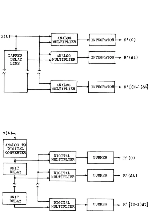
1. 4 Analog and Digital Autocorrelation Methods of
Spectral Measurement 22
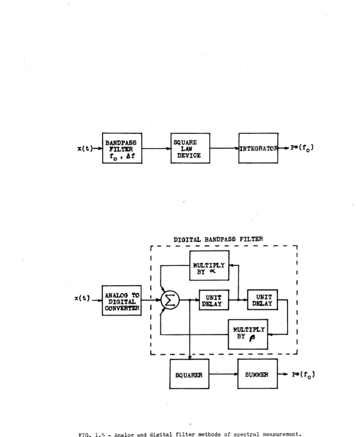
1. 5 Analog and Digital Filter Methods of
Spectral Measurement 23
1. 6 Ranges of Application of Various Spectral
Measurement Techniques 25
1. 7 The One-Bit Autocorrelation Method of
Spectral Analysis 28
2. 1 Effect of Sampling and Truncation of the
Autocorrelation Function
38
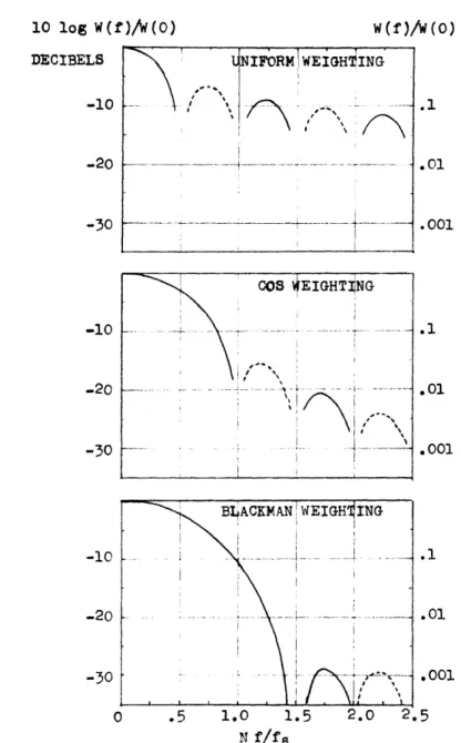
2. 2 Three Scanning Functions 41
2. 3 General Forms of the RMS Deviations of the
Autocorrelation Function and Power Spectrum 48 4. 1 The Switched- One-Bit Autocorrelation Radiometer 90
4. 2 The Switching Cycle 91
5. 1 Radio-Frequency Portion of the Deuterium-Line
Detection System 99
5. 2 Circuitry Used in the Deuterium-Line Receiver
to Perform the Clipping Operation 109
5. 3 Sampling Configuration Used in the
x
LIST OF ILLUSTRATIONS (Continued)
Figure Page
5. 4 Effect of Large Gain Changes Upon the
Measured Spectrum 110
5. 5 Basic Block Diagram of a One-Bit Digital
Correlator 113
5. 6 Digital Correlator Used for the Deuterium-Line
and Zeeman Experiments 119
5. 7 Circuit Diagram of a High-Speed Correlator
Channel 121
6. 1 Block Diagram of Computer Simulation
Program 129
6. 2 Results of Computer Simulated Autocorrelation
Function Measurements 133
6. 3 Results of Computer Simulated Spectral
Measurements 135
6. 4 Procedure for Producing a "Known"
Power Spectrum 141
6. 5 Procedure Used to Measure
IH(f)
{
1416. 6 Results Pertinent to Section 6. 3 144
6. 7 Artificial Deuterium-Line Generator 147
6. 8 Artificial Deuterium-Line Results 149
6. 9 Experimental and Theoretical Sensitivity of a
Conventional Dicke Radiometer Compared with 157 a One-Bit Autocorrelation Radiometer
xi
LIST OF ILLUSTRATIONS (Continued)
Figure Page
7. 1 Configuration for the Deuterium-Line
Experiment 164
7. 2 Effects of a Spatially-Varying Hydrogen
164 Optical Depth
7. 3 Results of the Deuterium-Line Experiment 172 8. 1 Results of Zeeman Observations in the Cas A
Radio Source 179
8. 2 Results of Zeeman Observations in the Taurus A
Radio Source 180
LIST OF TABLES
Table Page
1. 1 Comparison of Two One-Bit Methods of
Autocorrelation Function Measurement 31
2. 1 Properties of Three Weighting Functions 40 6. 1 Results of Computer Simulation Experiment
-Autocorrelation Functions 132
6. 2 Results of Computer Simulation Experiment
-Power Spectra 134
6. 3 Autocorrelation Function RMS Deviation 136
6. 4 Spectral RMS Deviation 138
6. 5 Analysis of the RMS Deviation of the
Deuterium-Line Data 155
xii
GLOSSARY
TIME FUNCTIONS
A stationary, ergodic, random time function having Gaussian statistics.
The function formed by infinite clipping of x(t). That is, y(t)
=
1 when x(t) > 0 and y(t) = .1 when x(t) < 0.FREQUENCY AND TIME
Due to their rather standard usage in both communication theory and radio astronomy, the symbols, T and - , symbolize different quantities in different sections of the paper. In the first 3 chapters, T is a time interval and t is the autocorrelation function delay variable. In the last 6 chapters, T is temperature and t is either optical depth or observation time. Some other frequency and time variables are the following:
At, k, K, ft
A'r, n, N' s
The time function sampling interval is At . A sample of the time function, x(t), is x(kAt) where k is an integer. The total number of
samples is K. The sampling frequency is ft = 1/At . In most cases At and ft will be chosen equal to A
t
and f , respectively.The autocorrelation function sampling interval is AT . The samples of the autocorrelation function are R(nAt) where n is an integer going from 0 to N-1. The reciprocal of At
is f s x(t)
I -~r-w.inI.Nnrrn - ----
,~-xiii
Af The frequency resolution of a spectral measurement (see Section 1. 3). It will be
approximately equal to 1/N-At.
B1 , B2 0 The 1 db and 20 db bandwidths of a
radio-meter. The spectrum is analyzed with resolution, A f , in the band, B The sampling frequencies,
ft
and f . are often chosen equal to 2B2 0.f A known combination of local oscillator 0
frequencies.
AUTOCORRELATION FUNCTIONS
R(t) The true autocorrelation function of x(t).
R "(T) A statistical estimate of R(t) based upon unquantized or many-bit samples of x(t)
p(t) or
px(T)
The true normalized autocorrelation function;p(t)
=
R(r)/R(0)."(T) A statistical estimate of p(T) based upon unquantized or many-bit samples of x(t) p'(-) or p t) A statistical estimate of p(T) based upon
one-bit samples of y(t) .
p (t) The true normalized autocorrelation function
of y(t) .
p' A statistical estimate of py(T) based upon
y s
I
=ZMtVW_ --- W ". . 11, , I I I __ t- - --- '
-xiv
POWER SPECTRA
(The power spectrum is defined in Section 1. 2) P(f) The true power spectrum of x(t)
P"(f) A statistical estimate of P(f) based upon unquantized or many-bit samples of x(t) P*(f) The expected value of P"(f)
p(f) The true normalized power spectrum;
p(f) = P(f)/R(O).
p"'(f) A statistical estimate of p(f) based upon many-bit or unquantized samples of x(t)
p'(f) A statistical estimate of p(f) based upon one-bit samples of y(t)
p*(f) The expected value of p'(f) and p''f). p'(f) c The normalized spectral estimate produced
by a one-bit autocorrelation radiometer when its input is connected to a comparison noise source.
p'(f) A normalized estimate of the receiver power transfer function, G(f) . It is the spectral estimate produced by a one-bit autocorrelation radiometer when the input spectrum and
receiver noise spectrum are white.
3p'(f) The estimate of the difference spectrum that is determined by a switched radiometer; 3p'(f)
=
p'(f) - p'(f)xv
TEMPERATURES
Ta(f) The power spectrum available at the antenna
terminals expressed in degrees Kelvin. Tr(f) The receiver noise temperature spectrum. T(f) The total temperature spectrum referred to
the receiver input. T(f) = T a(f) + Tr(f)
Tc(f) The spectrum of the comparison noise source.
Tav The frequency-averaged value of T(f). The average is weighted with respect to the receiver power transfer function, G(f) Ta av The frequency-averaged value of T a(f). Tc av The frequency-averaged value of
Tc(f) + Tr(f)
Tr av The frequency-averaged value of Tr (f)
3T The unbalance temperature; 3T T - T
av av av c av
RMS DEVIATIONS
A
ar
with two subscripts will be used to denote an RMS deviation of a statistical estimate. The first subscript will be a P, R, p, or pand indicates the variable to which the RMS deviation pertains. The second subscript will be a 1 or an m and indicates whether the statistical estimate is based upon one-bit or many-bit samples. Thus, for example, Crp1 is the RMS deviation of p'(f) , the one-bit
xvi
a single subscript and a prime or double prime indicating whether one-bit or many-bit samples are referred to. For example, c'(f)
p is a statistical estimate of cr (f)
MISCELLANEOUS
w('r) The function that is used to weight: the auto-correlation function; see Section 2. 2.
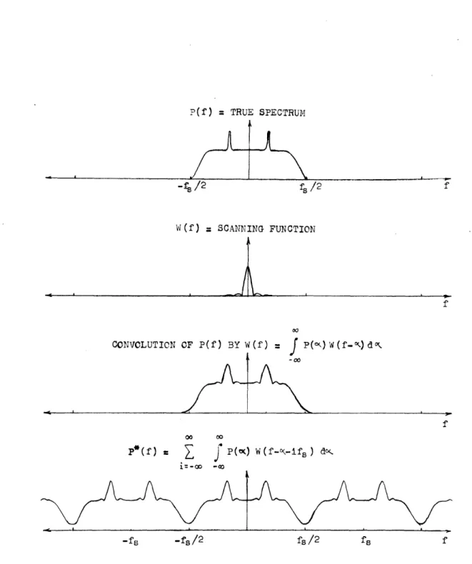
W(f) The spectral scanning or smoothing function. It is the Fourier transform of w('L);
see Figure 2. 2
G(f+f0) The receiver power transfer function. The spectrum at the clipper input, P(f) , is equal to G(f+f ) times the input temperature
spectrum, T(f+f0).
SPECIAL SYMBOLS
x(t) A line over a variable indicates that the
statistical average is taken. See Equation 1. 1.
P*(f) An asterisk superscript on a spectrum indi-cates that it has been smoothed and is
repeated about integer multiples of the sampling frequency. This operation is discussed in Section 2. 2.
Tt(f) The one-bit autocorrelation radiometer pro-duces a statistical estimate of an input tempera-ture spectrum such as T(f) . The statistical average or expected value of this estimate is equal to Tt(f) . The relationship between T(f) and Tt(f) is discussed in Section 4. 2-1. Under proper conditions, such as a sufficiently fast
sampling rate, Tt(f) is simply a smoothed version of T(f) .
I i~E~EE~II III -
-1~
CHAPTER 1
INTRODUCTION
This report can be divided into three parts which comprise Chapters
1 -2 - 3, 4 -5, and 6 - 7 - 8, respectively.
1) A technique for the measurement of the power spectrum and autocorrelation function of a Gaussian random process is presented. This technique, which will be referred to as "the one-bit autocorrelation method, " has the property that it is easily performed digitally; hence, the accuracy and flexibility associated with digital instrumentation is achieved. The technique is a multichannel one; that is, many points
on the spectrum and autocorrelation function can be determined at one time. A limitation is that the bandwidth analyzed must be less than
10 mc for operation with present-day digital logic elements.
2) The above technique will be applied to the problem of the measurement of spectral lines in radio astronomy. In Chapter 4 the composition and theoretical performance of a practical radio astronomy system utilizing the one-bit digital autocorrelation technique will be presented. The design of components of this system is discussed in Chapter 5.
3) The above system was constructed and extensive experimen-tal results are given. These results are of laboratory tests of the
2
system, an attempt to detect the galactic deuterium line, and an attempt to measure Zeeman splitting of the 21 cm hydrogen line.
The reader who is interested in the radio astronomy aspects of the report may wish to skip Chapters 2 and 3; the results of these two chapters are summarized in radio astronomy terms in Chapter 4.
The remainder of this chapter will be spent on some background material, a comparison of filter and autocorrelation methods of spec-tral measurement, a classification of specspec-tral measurement problems, and finally, a brief description of the one-bit autocorrelation method.
1. 1 STATISTICAL PRELIMINARIES
A brief presentation of some of the statistical techniques and terminology used in this paper will be given in this section. In addi-tion, some assumptions will be stated regarding the statistical nature
of the signals of interest. For an introduction to statistical communi-cation theory techniques, the reader is referred to Davenport
and
1 2
Root, Chapters 1 - 6 (109 pages) or Bendat, Chapters 1 and 2 (77 pages).
The type of signal which is -of interest in this paper is the random time function; that is, a signal whose sources are so numerous,
complicated, and unknown that exact prediction or description of the time function is impossible. Our interest is in the study of averages
__-3
of functions of the signal, in particular, the power spectrum, which will be defined in the next section.
A random variable, x , is the outcome of an experiment which (at least theoretically) can be repeated many times and has a result that cannot be exactly predicted. The flipping of a coin or the meas-urement of a noise signal at a given time are two such experiments. The outcome of a particular experiment is called a sample of the random variable; it is implied that there are a large number of sam-ples (although many samsam-ples may have the same value).
The random variable is described by a probability density function, p(x). The statistical average (this will sometimes be called the "mean") of a random variable will be denoted by a bar over the quantity being averaged, such as 3 . In terms of the probability density function, the statistical average of x is given by,
fx p(x) dx (1.1)
~00
In most signal analysis cases the random variable is a function of a parameter such as frequency or time. Thus, there is an infinite number of random variables, one for each value of the parameter. For each random variable there is a large number of samples. This two dimensional array of sample functions is called a random process and is illustrated on the following page.
(1)
x (t)
t t
0
Figure 1.1
The concept of a random process with time as the parameter is shown in Figure 1.1. For each value of time a random variable, xt9' is defined. Each random variable has an infinite number of samples,
x , x (2) (). The random process can also be described
0 (1) (2)
as having an infinite number of sample functions, x (t), x () . . . x(0(t). (The superscripts will be dropped when they are not needed for clarity.)
Statistical averages, such as 3F, are taken vertically through the random process array and may or may not be a function of time.
Time averages, such as,
T
- x(t) dt
T f 0
--are taken across the array and may or may not depend on the sample function chosen.
It will be assumed that signals whose power spectra we wish to measure are stationary and ergodic. By this it is meant that statis-tical averages such as xt ' t 2 and x t t +
t
are independent of0 0 0 0
the time, t , and are equal to the infinite time averages which, in turn, are independent of the particular sample function, i. e.,
T xt t Tlim T, Zo T f x (t) dt (1.2) 0 -T 2 lim 1 2 x ZT
J
x (t) dt (1.3) 0 -T T x x =--f
x(t) x(tt s) dt (1.4) t 0 t + Ir 0 T -+) oo 2 T TThese assumptions imply that the power spectrum does not vary with time (at least over the period of time that measurements are made). This is the usual situation in radio astronomy except for the case of solar noise.
Under the stationary and ergodic assumptions the sample functions of the random process have a convenient interpretation, each sample
6
function is a "record" or length of data obtained during different time intervals. The statistical average then has the interpretation as the average result of an operation repeated on many records.
The quantity, x t xt + , is called the autocorrelation function of
0 0
the signal. From Equation 1. 4 we see that under the stationary and ergodic assumption the autocorrelation function can also be expressed as an infinite time average. Because of the stationary assumption, xt t 0+ is not a function of t and the notation, R (T) or R(, )
o o
will be used to signify the autocorrelation function.
In words, the autocorrelation function is the (statistical or infinite time) average of the signal multiplied by a delayed replica of itself. R (o) is simply the mean square, x , of the signal, while R (00) is
2
equal to the square of the mean, K . It is easily shown that
R (o) > R_ () = R (-,r). The normalized autocorrelation function, PX (,), is equal to R ()/R (o) and is always less than or equal to unity.
The variance, a- 2 , of a random variable is a measure of its x
dispersion from its mean. It is defined as,
2 2
<r = (x - x 15
x
--L
7
The positive square root of the variance is the RMS deviation, r . The statistical uncertainty, A, of a random variable is the RMS deviation divided by the mean,
A x - (1.7)
As is often the case in the analysis of random signals, it will be assumed that the signal has Gaussian statistics in the sense that the joint probability density function, p (xt, xt+), is the bivariate Gaussian distribution, 1 2t R (o) 1 -
p Z
/2
x I x 2 2 (1.8) exp t Z - (ixtxt+r +X t+t -2. R (0) 11 P 2 -x xThis assumption is often justified by the central limit theorem (see Bendat , Chapter 3) which states that a random variable will have a
Gaussian distribution if it is formed as the sum of a large number of random variables of arbitrary probability distribution. This is usually true in the mechanism which gives rise to the signals observed in radio astr onomy.
8
1. 2 DEFINITION OF THE POWER SPECTRUM
The power spectrum is defined in many ways dependent on: 1) The mathematical rigor necessary in the context of the literature and application in which it is discussed, 2) Whether one wishes to have a single-sided or double-sided power spectrum (positive and negative frequencies, with P(-f) = P(f)
)}
3) Whether one wishes P(f)Af or2P(f) Af to be the power in the narrow bandwidth, Af.
In this paper, the double-sided power spectrum will be used since it simplifies some of the mathematical equations that are envolved.
The negative-frequency side of the power spectrum is the mirror image of the positive-frequency side; in most cases it need not be considered. In accordance to common use by radio astronomers and physicists, P(f) Af (or P(-f) Af ) will be taken to be the time average power in the bandwidth, Af, in the limit as Af -+ 0 and the
averaging time, T -+ 00 Thus, the total average power, PT, is
given by, 00 PT = P(f) df (1.9) 0
or
PT P(f) df (1. 10) T 0 0 L9
(if an impulse occurs at f = 0 , half of its area should be considered to be at f > 0 for evaluation of Equation 1. 9).
The statements of the preceding paragraph are not a sufficiently precise definition of the power spectrum because: 1) The relationship of P( f) to the time function, x(t) , is not clear, 2) The two limiting
processes (Af -+ 0, T -- 00 ) cause difficulty; i. e., what happens in the
limit to the product, TAf ?
A more precise definition of the power spectrum is obtained by defining P(f) as twice the Fourier transform of the autocorrelation function, R(-r), defined in the previous section. Thus, we have
00 -j 2 tf r
P(f) = 2 R(T ) e dr (1. 11)
-00
T
R(-)= Tlim 1 x(t) x(t + -) dt (1. 12)
The inverse Fourier transform relation gives,
R(T)
=f
P(f) cos 2,tfV df
(1.
13)
00
R(T) P(f) e df (1. 14)
10
This definition of the power spectrum gives no intuitive feeling as to the relation of P(f) to power. We must prove then, that this definition has the properties stated in the second paragraph of this
section. Equations 1. 9 and 1. 10 are easily proved by setting -r 0
in Equations 1. 12, 1. 13, and 1. 14. We find,
T R(o) = Tm
T
x2 (t) dt (1. 15) - T 00 R(o) = P(f) df (1. 16) 0The right-hand side of Equation 1. 15 is identified as P the total T'
average power. Power is used in a loose sense of the word; PT is the total average power dissipated in a one-ohm resistor if x(t) is the voltage across its terminals, otherwise a constant multiplier is
needed.
The proof that P(f)
Af
is the time average power in the band Af,as Af -* 0 and T -+ 0 is not as direct. Suppose that x(t) is applied
to a filter having a power transfer function, G(f). It can be shown by using only Equations 1. 11 and 1. 12 that the output power spectrum, P 0 (f) , is given by (see Davenport and Root, p. 182),
11
If G(f) is taken to be equal to unity for narrow bands of width, Af,
centered at +f and -f, and zero everywhere else, we find 00
P(f) df = P(f) Af (1.18)
0
as Af + 0. The left-hand side of Equation 1. 18 is simply the average
power out of the filter (using Equations 1. 15 and 1. 16) and, hence,
P(f) Af must be the power in the bandwidth Af.
1. 3 THE GENERAL FORM OF ESTIMATES OF THE POWER
SPECTRUM
The power spectrum of a random signal cannot be exactly measured by any means (even if the measurement apparatus has perfect accuracy); the signal would have to be available for infinite time. Thus, when the term "measurement of the power spectrum" is used, what is really meant is that a statistical estimate, P'(f), is measured.
The measured quantity, P'(f), is a sample function of a random process; its value depends on the particular time segment of the random signal that is used for the measurement. It is an estimate of P(f)
in the sense that its statistical average, PN(f) , is equal to a function, P*(f), which approximates P(f). The statistical uncertainty of P'(f) and the manner in which P*(f) approximates P(f) appear to be in-variant to the particular spectral measurement technique and will be briefly discussed in the next two paragraphs.
12
The function, P1(f), approximates P(f) in the sense that it is a smoothed version of P(f). It is approximately equal to the average value of P(f) in a band of width, Af, centered at f,
ftAf/2
P*(f) ~f P(f) df (1. 19)
f-Af /2
The statistical uncertainty, A , of P (f) , will be given by an p
equation of the form
A MP(f) -(f) 2
A P() - (1.20)
P*(f)
where T is the time interval that the signal is used for the measure-ment and
cX
is a numerical factor of the order of unity dependent on the details of the measurement.Equations 1. 19 and 1. 20 are the basic uncertainty relations of spectral measurement theory and appear to represent the best per-formance that can be obtained with any measurement technique (see Grenander and Rosenblatti 3 p. 129). Note that as the frequency
resolution, Af , becomes small making P"(f) a better approxima-tion of P(f) , the statistical uncertainty becomes higher
[
Pt(f) is a worse estimate of P*(f)1 . Optimum values of Af , with the cri-terion of minimum mean square error between P'(f) and P(f) are given by Grenander and Rosenblatt, pp. 153-155. In practice, Af13
one wishes to examine and T is chosen, if possible, to give the desired accuracy.
1. 4 COMPARISON OF FILTER AND AUTOCORRELATION METHODS OF SPECTRAL ANALYSIS
Two general methods have been used in the past to measure the power spectrum. These are the filter method, shown in Figure 1. 2 (a) and the autocorrelation method, shown in Figure 1. 2 (b). In this section the two methods will first be briefly discussed. A filter-method system that is equivalent to a general autocorrelation-method system will then be found.
This result serves two purposes: 1) It helps to answer the question, "Which method is best?" 2) An intuitive understanding of the filter-method system is quite easily achieved, while this is not true for the autocorrelation-method system. Therefore, it is often helpful to think of the autocorrelation-method system in terms of the equivalent filter-method system.
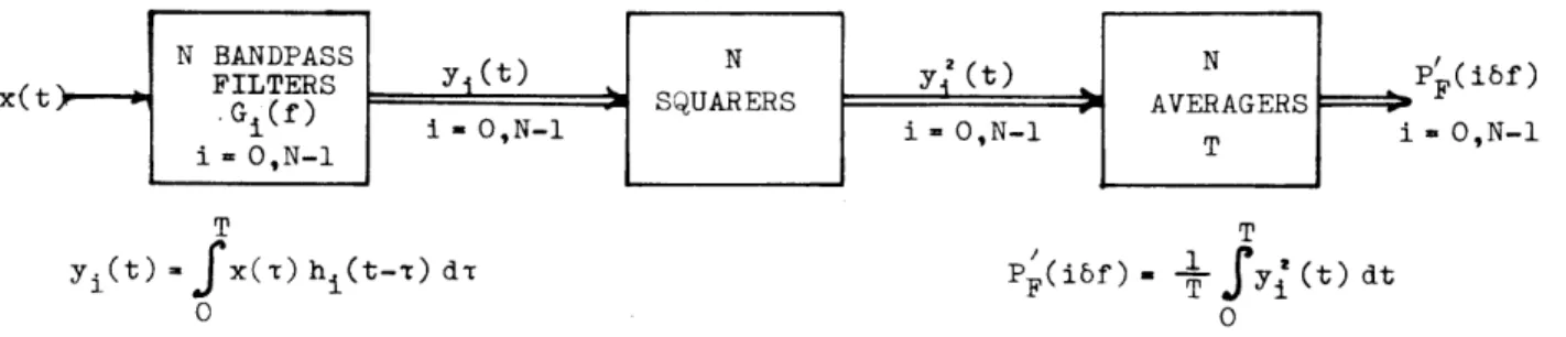
The filter-method system of Figure 1. 2 (a) is quite straight-forward. The input signal is applied in parallel to a bank of N bandpass filters which have center frequencies spaced by 6 f. The power transfer function of the i tth bandpass filter (i = 0 to N-1) is G.(f) [impulse
response, h.(t)] , which has passbands centered at i
f.
The N outputs of the filter bank are squared and averaged to give N numbers,N BANDPASS N y 2(t) N P/(ibf)
x(t FILTERS .Gi(f) SQUARERS AVERAGERS F
i -ON-1 i -ON-1 T i - ON-1 i = O,N-1 T T yj(t) = x(t) h (t-t) dt 0 T P (ibf) y 2(t) dt 0
FIG. 1.2(a) - Bandpass-filter method of spectral measurement.
N CHANNEL R(6) MULTIPLY BY R1(n )() SAMPLED
x(t) CORRLLATOR WEIGHTING R DATA A
n- O,N-1 FUNCTION n = ,N-1 FOURIER i= 09N-1
T w(t) N TRANSFORM
T
R I(nA1) -T0x(t) x(t+nA-) dt A/(ibf) = 24r N-1R (0) w(O)
+4A- R '(nat) w(nAr) cos 2ii6fn4t n=i
FIG. 1.2(b) - Autocorrelation method of spectral measurement.
H
4:-15
P
r
(i 3 f) , i = 0 to N - 1, which are estimates of the power spectrum, P(f), at f = i 3 f.The relation of the filter-method spectral estimate, P (i 5 f), to the input signal, x(t), is,
T T
P =
[if
x±rh (X-t)d
)
P
(i f) h tdt dX (1.21)0 0
which is the time average of the square of the convolution integral expression for .the filter output in terms of the input. It is assumed that x(t) is available for only a finite interval, T, and that the filter input is zero outside of this interval. The relation of P' (i 3 f) to the true spectrum is of the form of Equations 1. 19 and 1. 20 where
A
f is simply the filter bandwidth.The autocorrelation method of spectral analysis is based upon the expression (called the Wiener-Khintchin theorem) giving the power
spectrum as a Fourier transform of the autocorrelation function, R(t ). Indeed, this is the way we defined the power spectrum in Section 1. 2.
The expression is repeated below,
00 -2 g f
T
P(f) = 2 R( t ) e dr (1. 22)
-00
The autocorrelation function can be expressed as a time average of the signal multiplied by a delayed replica of itself,
16 T
R(T) = T f x(t) x(t+-t) dt (1.23)
-T
The operations indicated in Equations 1. 22 and 1. 23 cannot be per-formed in practice; an infinite segment of x(t) and an infinite amount of apparatus would be required. An estimate of R(T) at a finite number of points, T nAt, can be determined by a correlator which computes,
T
R (nA -r) x(t) x(t+nAr) dt (1.24)
0
A spectral estimate, P (i b f), can then be calculated as a modified Fourier transform of RE (nAt)
N-1
P (i f) = 2A T R (o) w(o) + 4At R'(nAt) n=1
(1. 25) w(nAt) cos (27i f nAt)
The numbers, w(nAt) , which appear in Equation 1. 25 are samples of a weighting function, w(T) , which must be chosen; the choice is dis-cussed in the next chapter. The weighting function must be even and have w(-r) = 0 for t> NAT; its significance will soon become apparent. In order to use all of the information contained in R'(nAt), 5f should be chosen equal to 1/ [ 2(N-1)At ]. This follows from application of the Nyquist sampling theorem; PX(iS f) is a Fourier transform of a function band-limited to (N-1) AT.
17
The relation of P F (i 5f) to the true power spectrum will again be of the form of Equations 1. 19 and 1. 20 where Af, the frequency
resolution, is approximately equal to 1/ [(N - 1) At ] . The calculation of the exact relation between Pt (i 5f) and P(f) will be the major topic of Chapter 2. Our major concern in this section is to relate P' (i 6f) and P (i sf).
It is shown in Appendix A that P' (i 3 f) will be equal to P' (i 5 f) for any common input, x(t), provided the filter responses and the
auto-correlation weighting function, w( t ), are related in a certain way. The only significant assumption that was required for this proof is that the duration of the data, T, be much longer than the filter time constants (or equivalently, N At
).
This requirement must be satisfied in practice in order to obtain a meaningful spectral estimate, and thus, it is not an important restriction.The required relation between the filter response and the auto-correlation weighting function is most easily stated in terms of Gi(f)
,
the power transfer function of the i tth filter, and W(f), the Fouriertransform of the weighting function,
00
W(f) = 2 w(T ) cos 2C ft dt (1.26) 0
The relation is,
00
G(f M W(f - i Ff-kfs) + W(f +i Ff +kfs) (1.27) k=-00
18
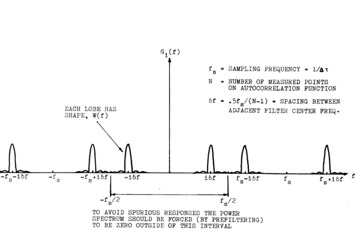
where f = I/Ar . This result is illustrated in Figure 1. 3; G.(f) S
consists of narrow bandpass regions, each having the shape of W(f), centered at +i
f,
f +if,
2f * i 3f, etc.It is thus obvious that the autocorrelation spectral measurement system has many spurious responses. It can be seen that these spurious responses will have no effect if the input power spectrum is restricted (by prefiltering) such that,
P(ft) W(f-f') df 1) df1 = 0 for
Jfj
> f /2 (1.28) -00This requirement, a necessary consequence of sampling of the auto-correlation function, is, of course, not required with the filter-method system since filters without spurious response are easily constructed.
If the requirement of Equation 1. 28 is met, the terms where k A 0
in Equation 1. 27 have no effect and an equivalent set of filter power transfer functions is given by,
G.(f) = W(f - i 3f) + W(f+i Ff) (1. 29) 1
Furthermore, if we consider only positive frequencies not close to zero, we obtain,
fs -isf -f
G (f)
EACHLOBEHA4
EACH LOBE HAS
SHAPE, W(f)
-f s/2
f = SAMPLING FREQUENCY = 1/AT
s
N = NUMBER OF MEASURED POINTS ON AUTOCORRELATION FUNCTION
bf .5fs/(N-1) - SPACING BETWEEN
ADJACENT FILTER CENTER FREQ.
(VA-
A
i6f I: -i5f
i6f f s ib
f s 1
s S+101
TO AVOID SPURIOUS RESPONSES THE POWER SPECTRUM SHOULD BE FORCED (BY PREFILTERING)
TO BE ZERO OUTSIDE OF THIS INTERVAL
FIG. 1.3 - The autocorrelation method of spectral measurement depicted in Fig. 1.2(b) is equivalent to the filter-array method of Fig. 1.2(a) if the i'th
filter (i=O .to N-1) has the power transfer function, Gi(f), shown above. W(f) is the Fourier transform of the autocorrelation weighting function, w('r).
kD
A--20
To summarize then, we have shown that the estimation of N points on the autocorrelation function (Equation 1. 24) followed by a modified Fourier transform (Equation 1. 25) is equivalent to an N-filter array spectral measurement system if Equation 1. 27 is satisfied. Each method estimates the spectrum over a range of frequencies, B = (N-1)3f
= f /2, with 5f spacing between points. If the autocorrelation method is used the spectrum must be zero outside of this range.
Note that the G.(f) which can be realized with practical filters is quite different than the equivalent G.(f) of an autocorrelation system (to the advantage of the filter system). The restriction on W(f) is that it be the Fourier transform of a function, w( 'r), which must be zero for t > N At . This restriction makes it difficult to realize an equiva-lent Gi(f) which has half-power bandwidth, Af, narrower than
2/(N AZt)
2 f (high spurious lobes result). No such restriction between the bandwidth, Af, and the spacing, 3f, exists for the filtersystem.
In most filter-array spectrum analyzers, 3f is equal to Af; that is, adjacent filters overlap at the half-power points. This cannot be done with the autocorrelation method; 3f will be .4 to .8 times A f dependent
on the spurious lobes which can be tolerated. This closer spacing gives a more accurate representation of the spectrum, but is wasteful in terms
of the bandwidth analyzed, B = (N-1) 5f, with a given resolution, Af. For this reasonit appears that 2 autocorrelation points per equivalent filter is a fairer comparison.
-WE
~-21
1. 5 CHOICE OF THE SPECTRAL MEASUREMENT TECHNIQUE
In the previous section we have compared the filter and autocorrela-tion methods of spectral analysis on a theoretical basis. The major result is that if we desire to estimate N points on the spectrum during one time interval, we may use either an N filter array as in Figure 1. 2(a) or a 2N point autocorrelation system as in Figure 1. 2(b). The estimates of the power spectrum obtained by the two methods are equiva-lent; there is no theoretical advantage of one method over the other.
Both methods of spectral analysis can be performed with both
analog and digital instrumentation as is indicated in Figures 1. 4 and 1. 5. In addition, if digital instrumentation is chosen, a choice must be made between performing the calculations in a general purpose digital com-puter or in a special purpose digital spectrum analyzer or correlator.
The digital filter method* shown in Figure 1. 5 deserves special mention as it is not too well known. The procedure indicated in the block diagram simulates a single-tuned circuit; the center frequency and Q are determined by a and 3 . The digital simulation of any analog filter network is discussed by Tou, 4 pp. 444-464. The digital filter method will be compared with the digital autocorrelation method later in this section.
I would like to thank M. J. Levin, M. I. T. Lincoln Laboratory, for pointing out this technique to me.
22
INTEGRATOR R' (0)
DELAY MULTIPLIER INTEGRATOR R'(4t)
LINE MU INTEGRATOR R' [(N- )At) x( t) ANALOG TO DIGITAL CONVERTER MULTPLIER- UER -+ '() UNIT DEL AY DIGIT AL
MULT IPLIER SUMMER -+R (A t )
UNT
DEL AY
SDIGITAL ESUMMER R[(N-1)At]
23
BANDPASS SQUAREP*
xt
)-+ nITER - - LAW NER O +P(f 0fo , s f DEVICE
DIGITAL BANDPASS FILTER
MULTIPLY +
BY 0
x(t) -*DIGITALDEA ANAG T UNIT UNIT
DEA
CONVERTERDEA DLY
MULTIPLY
BY.
SQUARER ' SUMMER -+P*(fe )
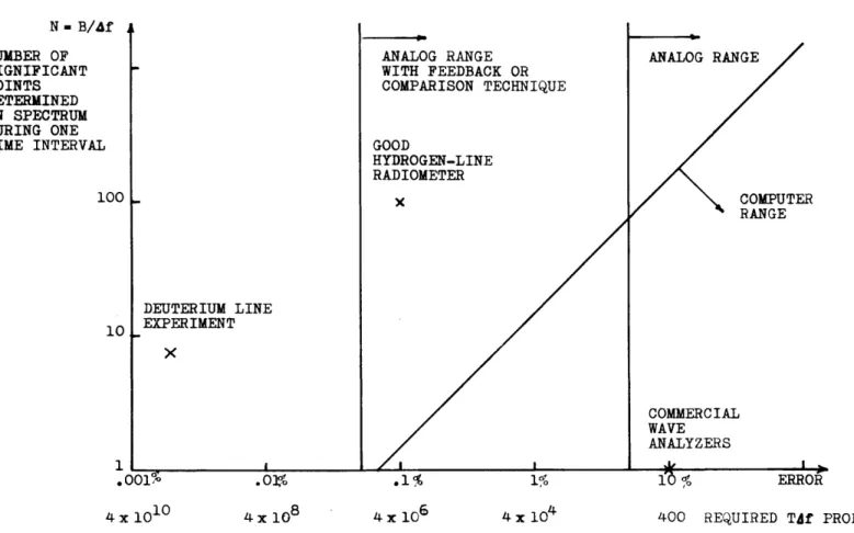
24-A way of classifying spectral measurement problems into ranges where various techniques are applicable is indicated in Figure 1. 6. The ordinate of the graph is N, the number of significant points which are determined on the spectrum and the abscissa is the percent error which can be tolerated in the measurement.
The error in a spectral measurement is due to two causes: 1) The unavoidable statistical fluctuation due to finite duration of data, 2) the erro r caused by equipment inaccuracy and drift. The statistical
fluctuation depends through Equation 1. 20 on the frequency resolution-observation time product, T
A
f. The value of T Af that is required for a given accuracy is plotted on the abscissa of Figure 1. 6.The error due to equipment inaccuracy and drift limits the range of application of analog techniques as is indicated in Figure 1. 6. These ranges are by no means rigidly fixed; exceptions can be found. However, the line indicates the error level where the analog instrumentation
becomes exceedingly difficult.
The range of application of digital-computer spectral analysis is limited by the amount of computer time that is required. The line that
a
drawn represents one hour computer time on a high speed digital com-puter performing 104 multiplications and 104 additions in one second. It is interesting that the required computer time is not highly dependent on whether the autocorrelation method or the filter method is program-med on the computer. This will be shown in the next paragraph.k
N - B/Af NUMBER OF SIGNIFICANT POINTS DETERMINED ON SPECTRUM DURING ONE TIME INTERVAL 100
L-10
11
DEUTERIUM LINE EXPERIMENT x .0015 ANALOG RANGE WITH FEEDBACK OR COMPARISON TECHNIQUE GOOD HYDROGEN-LINE RADIOMETER x 1% ANALOG RANGE COMPUTER RANGE COMMERCIAL WAVE ANALYZERSfO
% ERROR 4x 10 10 . or.4 x 108 4 x 10⁶ 4 x 10⁴ 400 REQUIRED TAf PRODUCT
FIG. 1.6 - Range of application of various spectral measurement techniques.
kji
26
Examination of Figure 1.4 reveals that one multiplication and one addition are required per sample per point on the autocorrelation func-tion. The sampling rate is 2B, and ZN autocorrelation points are required for N spectrum points; thus, 4NB multiplications and addi-tions per second of data are required. A similar analysis of the digital-filter method of Figure 1. 5 indicates 3 multiplications and 3 additions per sample per point on the spectrum are required. This gives 6NB multiplications per second of data. The number of seconds of data that is required is given by solving Equation 1. 20 for T in terms of the statistical uncertainty, A , and the resolution Af. This gives
2
T = 4/(A Af) where the numerical factor,
a
, has been assumed p2 2 2 2
equal to 2. We then find 16 N /A and 24N /A as the total
p p
number of multiplications and additions required with the autocorrelation method and filter method, respectively. Because of the square
de-pendence on N and A , the computer time increases very rapidly to the left of the one-hour line of Figure 1. 6.
Some additional considerations concerning the choice of a spectral analysis technique are as follows:
1) If analog instrumentation is used, the filter method appears to be more easily instrumented and, of course, does not require the
Fourier transform. The bandpass filter, squarer, and averager can be realized with less cost and complexity than the delay, multiplier,
and averager required by the autocorrelation system. Analog
correla-tion may be applicable to direct computation of autocorrelation functions and cross-correlation functions, but not to spectral analysis.
27
2) Analog instrumentation is not suited for spectral analysis at very low frequencies (say below one cps) although magnetic tape speed-up techniques can sometimes be used to advantage.
3) Digital instrumentation cannot be used if very large band-widths are involved. At the present time, it is very difficult to digitally
process signals having greater than 10 mc bandwidth.
4) If digital instrumentation or a computer is used for the spectral analysis, there seems to be little difference between the auto-correlation method and the filter method if the same degree of quantiza-tion (the number of bits per sample) can be used. This is evident from the computation of the required number of multiplications and additions earlier in this section. However, if the autocorrelation method is used,
only one bit per sample is necessary and the multiplications and additions can be performed very easily. This method will be discussed in the next section.
1. 6 THE ONE-BIT AUTOCORRELATION METHOD OF SPECTRAL ANALYSIS
The one-bit autocorrelation method of spectral analysis, as it is used in this paper, is presented with explanatory notes in Figure 1. 7.
Most of the remainder of the paper will be concerned with the analysis of this system, its application to radio astronomy, and experimental results obtained with this system.
The key "clipping correction" equation given in Figure 1. 7 was 5
28
THE ONE-BIT AUTOCORRELATION METHOD OF SPECTRAL ANALYSIS
RESTRICTIONS ON THE INPUT SIGNAL, x(t):
x(t) 1) MUST BE A GAUSSIAN RANDOM SIGNAL
2) MUST HAVE A BAND-LIMITED POWER SPECTRUM,
P(f)=O for Ifl >B
CLIPPING OPERATInN DEFINED AS: CLIPPER
y(t) :1 when x(t) >'O
y(t) a -1 when x(t) O
---
y(t)---SAMPLING RATE = 2B u 1/-t
SAMPLER
EACH SAMPLE IS A ONE-BIT DIGITAL NUMBER
--- y(kt)
---ONE-BIT FUNCTION OF CORRELATOR DESCRIBED BY:
DIGITAL P'(nat) =I t y(kAt) y(kht + nt)
CORRELATOR n- knl y- yK
CORRELATION TAKES PLACE FOR T SECONDS. ?'(nat) IS THEN READ OUT OF THE CORRELATOR AB IS FED INTO A COMPUTER WHERE THE FOLLOWING TAKES PLACE:
THE ERROR CAUSED BY CLIPPING IS REMOVED BY:
f(nAt) a sin
fr(nAt)]
THE SPECTRAL ESTIMATE, p'(f), IS GIVEN BY:
N-1
p'(f) . 26t (O)w(O)+2 f(nAt)w(nat)
..- . .- - .. - -.--- -- - -- -- -. - -. . cos2-irfnAt
THE RESULT, p'(f), IS A STATISTICAL ESTIMATE
OF THE POWER SPECTRUM, P(f), NORMALIZED TO
HAVE UNIT AREA AND CONVOLVED WITH A FUNCTION OF BAND4IDTH, &f~- 2B/N. I. . . CLIPPING CORRECTION -- --- P.(nat) FOURIER TRANSFORM p'(f) F:(. 1.7
29
data processing, the present use of the relation was certainly not foreseen; it was simply a means of finding the correlation function at the output of a clipper when the input was Gaussian noise. The use of the relation for the measurement of correlation functions has been
6 7 8
noted by Faran and Hills, Kaiser and Angell, and Greene. The principle contributions of this paper are: 1) The investigation of the mean and statistical uncertainty (as in Equation 1. 20) of a spectral
estimate formed as indicated in Figure 1. 7, 2) The application of this technique to the measurement of spectral lines in radio astronomy.
It should be understood that the spectral measurement technique as outlined in Figure 1. 7 applies only to time functions with Gaussian statistics (as defined by Equation 1. 8). Furthermore, only a normalized autocorrelation function and a normalized (to have unit area) power
spectrum are determined. The normalization can, of course, be re-moved by the measurement of an additional scale factor (such as
00
P(f) df). These restrictions do not hamper the use of the system 0
for the measurement of spectral lines in radio astronomy.
Recently, some remarkable work which removes both of the above restrictions has been done in Europe by Veltmann and Kwackernaak,
9
10
and Jespers, Chu, and Fettweis. These authors prove a theorem which allows a one-bit correlator to measure the (unnormalized)
theorem and the measurement procedure are summarized in Appendix B. A comparison of this procedure with that of Figure 1. 7 is outlined in Table 1,.1
It is suggested (not too seriously) that the above mentioned method of measurement of autocorrelation functions be referred to as the ElB (European one-bit)method, while the procedure of Figure 1. 7 be referred to as the AlB (American one-bit) method. Any hybrid of the two pro-cedures could be called the MA1B method for mid-Atlantic one-bit or modified American one-bit dependent on which side of the Atlantic
one is on.
-
31
TABLE 1.1
COMPARISON OF TWO ONE-BIT METHODS OF AUTOCORRELATION FUNCTION MEASUREMENT
AlB METHOD ElB METHOD
(Fig. 1. 7) (Appendix B)
Restrictions on Must have Gaussian Must be bounded by
signal, x(t) statistics. iA.
Differences in 1) Clipping level is 1) Clipping level is
ran-procedure 0 volts. domly varied from
-A to +A. 2) SIN correction of 2) No correction.
one-bit autocor-relation function.
Mean of result Normalized autocor- Unnormalized autocor-relation function. relation function.
RMS deviation Increased by less than A preliminary analysis
of result com- 7t
/2.
indicates increasepared with RMS depends on
deviation of A2
many-bit
32
CHAPTER 2
THE AUTOCORRELATION FUNCTION METHOD OF MEASURING POWER SPECTRA
2. 1 INTRODUCTION
The theory of measuring the power spectrum through the use of the autocorrelation function will be presented in this chapter. We will start with the defining equations, repeated below, of the power spectrum, P(f) , of a time function, x(t)
P(f) = 2
f
R(x)-j
ZrfT dx (2. 1) -00 T R(,r) T lim T x(t) x(t+-r) dt (2. 2) T -+1 oo Z T f - TIf these equations are examined with the thought of measuring P(f) by directly performing the indicated operations, the following conclusions are reached:
1) In practice,- the time function is available for only a finite time interval, and thus the limits on -r and t cannot be infinite as in Equations 2. 1 and 2. 2. Both the time function and the autocorrelation function must be truncated.
331
2) If the operation of Equation 2. 2 is to be performed by a finite number of multipliers and integrators, then
T
cannot assume a continuous range of values. The autocorrelation function, R(-) ,must be sampled; that is, it will be measured only for r = nAT where n is an integer between 0 and N-1.
3) If digital processing is to be used, two more modifica-tions must be made. The time function will be sampled periodically
giving samples, x(kAt) where k is an integer between 1 and (KtN), the total number of samples. Each of these samples must be quantized. If its amplitude falls in a certain interval (say x - A/Z to x + A/2)
a discrete value (x ) is assigned to it. It will be shown in the next chapter that the quantization can be done extremely coarsely; just two intervals, x(kAt) < 0 and x(k At)> 0 can be used with little effect on the spectral measurement.
These considerations lead us to define the following estimates of the power spectrum and autocorrelation function,
0O
P "(f) &2A Z R"(nAr) w(nAt) e-j ZTf nA-t (2.3) n= -oo
K
R I t(n A ) x(kat) x(k At + Jn{ A T) (2. 4)
k=l
The function, w(nAr) , is an even function of n , chosen by the observer, which is zero for I ni > N and has w(0) = 1. It is included in the
34
definition as a convenient method of handling the truncation of the autocorrelation function measurement; R"(n&r) need not be known for
InJ
> N. The choice of w(nAt) will be discussed in Section 2. 2- 2.The estimates given by Equations 2. 3 and 2. 4 contain all of the modifications (sampling and truncation of the time function and auto-correlation function) discussed above except for quantization of sam-ples which will be discussed in the next chapter. We will call these estimates the many-bit estimates (denoted by a double prime) as contrasted with the one-bit estimates (denoted by a single prime) of the next chapter.
The main objective of this chapter will be to relate the many-bit estimates, P"(f) and R"(nAT) to the true values, P(f) and R(nAr). Many of the results will be applicable to the discussion of the one-bit estimates in the next chapter; other results are found for the sake of comparison with the one-bit results.
It is assumed, of course, that x(t) is a random signal having Gaussian statistics. The estimates, P"(f) and R"I(nAt), are therefore random variables since they are based on time averages (over a finite interval) of functions of x(t). The particular values of P"(f) and R(nA-T) depend on the particular finite time segment of x(t) that they are based on.
The mean and variance of P"(f) and R"(f) describe, for our pur-poses, their properties as estimates of P(f) and R(nAl). The mean, R"(nAr), of R"(nAt), is easily found,
35
KR t (nA) = x(kAt) x(kAt + In! AT) (2. 5) k=1
=
R(nA t)
(2.6)where we have made use of the fact that the statistical average of
x(kAt) x(kAt +
In!
AT) is simply R(nAt). R'(nAt) is called an unbiased estimate of R(nAt).The mean of P (f) is also easily found by taking the statistical average of both sides of Equation 2. 3 and using Equation 2. 6. Defining P'(f) as the mean of P"t(f), we find,
00
P'(f) = P(f) =2ZA
R(n A T) w(nAt) e -2cfnAt
(2.7)
n
=-
oo
If it were not for the sampling and truncation of R(-r) , P*(f) would
simply be equal to P(f) and,hence, P t(f) would be an unbiased estimate of P(f) . The relationship of P*(f) to P(f) will be discussed in the
next section. In later sections, the variances of P"(f) and R"(nAt) will be found.
Much of the material presented in this chapter is contained in a different form in the small book, The Measurement of Power Spectra, by Blackman and Tukey. 1 For the sake of completeness this material has been included here. An extensive bibliography to past work in this field is given by Blackman and Tukey.