HAL Id: hal-00317574
https://hal.archives-ouvertes.fr/hal-00317574
Submitted on 7 Sep 2004
HAL is a multi-disciplinary open access
archive for the deposit and dissemination of
sci-entific research documents, whether they are
pub-lished or not. The documents may come from
teaching and research institutions in France or
abroad, or from public or private research centers.
L’archive ouverte pluridisciplinaire HAL, est
destinée au dépôt et à la diffusion de documents
scientifiques de niveau recherche, publiés ou non,
émanant des établissements d’enseignement et de
recherche français ou étrangers, des laboratoires
publics ou privés.
over Svalbard
N. Ivchenko, M. H. Rees, B. S. Lanchester, D. Lummerzheim, M. Galand, K.
Throp, I. Furniss
To cite this version:
N. Ivchenko, M. H. Rees, B. S. Lanchester, D. Lummerzheim, M. Galand, et al.. Observation of O+
(4P-4D0) lines in electron aurora over Svalbard. Annales Geophysicae, European Geosciences Union,
2004, 22 (8), pp.2805-2817. �hal-00317574�
4Center for Space Physics, Boston University, Boston, Massachusetts, USA 5Atmospheric Physics Laboratory, University College London, UK
Received: 12 September 2003 – Revised: 7 May 2004 – Accepted: 12 May 2004 – Published: 7 September 2004
Abstract. This work reports on observations of O+lines in aurora over Svalbard, Norway. The Spectrographic Imag-ing Facility measures auroral spectra in three wavelength intervals (Hβ, N+2 1N(0,2) and N
+
2 1N(1,3)). The oxy-gen ion4P-4D0multiplet (4639–4696 ˚A) is blended with the N+2 1N(1,3) band. It is found that in electron aurora, the brightness of this multiplet, is on average, about 0.1 of the N+2 1N(0,2) total brightness. A joint optical and incoherent scatter radar study of an electron aurora event shows that the ratio is enhanced when the ionisation in the upper E-layer (140–190 km) is significant with respect to the E-layer peak below 130 km. Rayed arcs were observed on one such oc-casion, whereas on other occasions the auroral intensity was below the threshold of the imager. A one-dimensional elec-tron transport model is used to estimate the cross section for production of the multiplet in electron collisions, yielding 0.18×10⁻¹⁸cm2.
Key words. Meteorology and atmospheric dynamics
(air-glow and aurora) – Ionosphere (particle precipitation)
1 Introduction
Aurora is produced when atmospheric atoms and molecules excited in collisions with energetic particles (either directly or through a chain of chemical reactions) emit light as they undergo transitions to lower energy states. The auroral spec-trum depends on the composition of the upper ionosphere, and the energy distribution functions of the precipitating par-ticles. Understanding the processes shaping the spectrum is important to be able to characterize the auroral precipitation from ground-based spectroscopic observations. While in situ satellite and rocket particle instruments provide an accurate and direct measurement of the energy distribution functions, they suffer from spatial-temporal ambiguity. Information de-rived from the inversion of auroral emission spectra is coarser Correspondence to: N. Ivchenko
and more indirect in nature, but, on the other hand, it records the evolution of the precipitation at one location.
Spectral features originating from various excited states of the atmospheric constituents exhibit different dependences on the precipitation energy spectra. For example, the height-integrated emission rate of N+2 first negative bands is often treated as proportional to the height-integrated N2ionization rate and thus proportional to the total energy flux in electron aurora (e.g. Semeter et al., 2001). The forbidden emissions, such as [OI] 5577 and 6300, on the other hand, also depend on the characteristic energy of the accelerated electrons. At lower altitudes, the metastable states are collisionally deac-tivated, so higher energy electrons, which penetrate deeper in the atmosphere, are less efficient in producing those emis-sions. Ratios of emissions in different spectral lines have been used to infer the energies of the electrons. Typically, forbidden oxygen emissions are used together with the N+2 allowed emissions (Vallance Jones et al., 1987) – though their excitation mechanisms are not always easy to under-stand (Meier et al., 1989). It was also shown that oxygen emissions, which were allowed, are dependent on the energy of the incident electron precipitation (e.g. Lummerzheim, 1987; Lummerzheim et al., 1990).
We present a study of the O+4P-4D0multiplet, observed together with the N+2 1N(0,2) and N+2 1N(1,3) bands in au-rora excited primarily by electron precipitation. This mul-tiplet has long ago been identified (e.g. Chamberlain, 1961; Vallance Jones, 1974), but received little attention. The lines of the multiplet blend with the N+2 1N(1,3) band, being of a comparable strength. In studying the N+2 first negative emissions in twilight conditions resonant scattering of sun-light can be important for low solar depression angles (e.g. Remick et al., 2001). The scattering is most pronounced for bands originating from the ground vibrational state of the N+2 molecule, and the N+2 1N(1,3) band is the brightest of the 1N bands originating from a vibrationally excited state. The in-tensity ratio of N+2 1N(1,3) to N+2 1N(0,2) have been stud-ied in relation to the vibrational excitation of N+2 produced by ionization in proton impact (Vallance and Jones, p. 176, 1974), and the contribution for O+lines should be properly
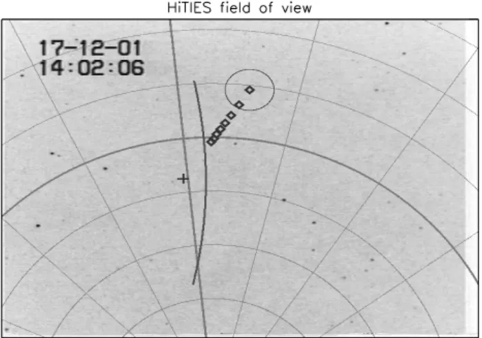
Fig. 1. Fields of view of the SIF instruments and the ESR. The cross
is the direction of the magnetic zenith. The ESR beam is shown as the circle at 100 km altitude. Diamonds show the centre of the beam at altitudes between 100 km and 240 km with 20 km spacing.
quantified. The companion paper (Ivchenko et al., 2004) studies the mechanisms of the excitation of the O+ lines in proton aurora. Finally, the multiplet feeds the 539 ˚A UV line, which is relevant for space-borne auroral spectroscopy.
By combining the spectral, imaging and incoherent scatter data, we show that the ratio of the multiplet intensity to the first negative emissions varies in different types of aurora. Enhanced O+ intensities coincide with enhanced ionisation
between 140 and 190 km. By inverting the radar electron concentration altitude profiles, the characteristic energy of the precipitation is inferred and related to the ratio of O+and N+2 1N(0,2) brightnesses, which is found to decrease with the electron energy. Assuming a simple functional form for the energy dependence of the cross section, a one-dimensional electron transport model is used to arrive at the absolute value of the cross section for production of the multiplet.
2 Instrumentation and Data
2.1 Spectrographic Imaging Facility
The Spectrographic Imaging Facility (SIF) is a combina-tion of ground-based optical instruments, jointly operated by the University of Southampton and University College, Lon-don. The facility consists of the High Throughput Imaging Echelle Spectrograph (HiTIES), developed at Boston Uni-versity (Chakrabarti et al., 2001), two photometers and a nar-row field (12×16◦) auroral imager. SIF is located at the au-roral station in the Adventdalen, near Longyearbyen, Sval-bard, Norway (78.203◦N, 15.829◦E). The instruments are co-aligned in the direction of the magnetic zenith. The high-latitude location provides a unique opportunity to study au-rora almost 24 h a day during the winter. The location is 7 km north of the EISCAT Svalbard Radar. A comprehensive de-scription of the SIF is provided elsewhere (McWhirter et al.,
2003; Lanchester et al., 2003), so only the information essen-tial for this study is given here.
HiTIES is a spectrograph designed specifically for auroral and airglow studies. Light from the slit covering 8◦in the
sky (see Fig. 1) is collimated, diffracted by echelle grating, and reimaged onto the detector. By using high diffraction orders close to the blaze angle of the grating, high spectral resolution is achieved, together with high throughput. The overlapping diffraction orders are separated by a mosaic of interference filters. The layout of the mosaic determines the spectral and spatial coverage of the instrument. In the data used here, a three-panel mosaic was used, with all the panels extended to cover the whole angular range of 8◦ centred at the magnetic zenith, while selecting spectral intervals con-taining the Hβ, N+2 1N(0,2) and N+2 1N(1,3). The detector
used during the winter of 2001/2002 was the Microchannel Intensified CCD (Fordham et al., 1991), on loan from the astronomy group at University College, London. The main advantage of the detector is the photon-counting capability and very low dark count rate and lack of read-out noise.
The spectral resolution of the HiTIES is determined by the width of the slit, which also controls the amount of light en-tering the instrument. A reasonable compromise in slit width of 0.27 mm (corresponding to about 3 arcminutes on the sky) resulted in a 0.8 ˚A FWHM instrument function. Typical inte-gration times are between 10 and 60 s. All spectra analyzed in this work are integrated over a 2◦-long part of the slit cen-tred at the magnetic zenith.
The Solar Fraunhofer absorption spectrum is used for wavelength calibration of each HiTIES spectral panel. For intensity calibration a “flat field” lamp is used together with the photometers. In 2002/2003 an absolute calibration was carried out with the Tungsten lamp used for calibration of the meridian scanning photometers. The 2001/2002 calibration is referenced to this standard by means of the photometers. 2.2 EISCAT Svalbard Radar
Data from the EISCAT Svalbard Radar (ESR) are used here to characterize the electron precipitation. The ESR incoher-ent scatter radar (Wannberg et al., 1997) measures a number of ionospheric parameters over a range of altitudes. A high frequency signal is transmitted and scattered by electrons in the ionospheric plasma. By analysing the Doppler broadened profiles of the spectrum of the scatter, four parameters can be derived from the data directly: electron number density, plasma velocity, ion and electron temperatures.
2.3 Data and analysis
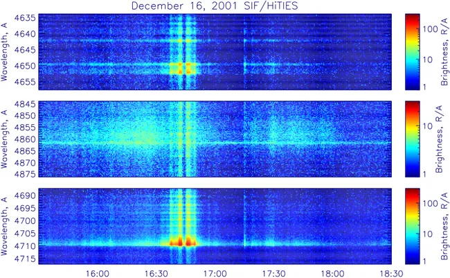
An example of the SIF observation of mixed electron and proton aurora from 16 December 2001 is shown in Fig. 2. Three hours of 30-s integration spectra taken in the direction of the magnetic field are presented. In the top panel, the most prominent features throughout the interval are the O+lines at 4641.8 ˚A and 4649.1 ˚A. Somewhat weaker is the emission between 4652 ˚A and 4650 ˚A, corresponding to the blended
Fig. 2. Overview plot of the SIF data from 15:30–18:30 UT, 16 December 2001. The panels show the time dependence of the spectra of the
N+2 1N(1,3) band, Hβ, and the N+2 1N(0,2) band, respectively, as measured by HiTIES.
N+2 1N(1,3) emission with the head at 4651.8 ˚A and another O+line at 4650.8 ˚A. Even fainter is the O+line at 4638.9 ˚A.
At 16:40–16:50 UT there is intense aurora, and the rotational structure of the N+2 1N(1,3) band is seen to extend throughout the spectral interval to the blue color of the band’s head.
The second panel shows the spectral interval 4843 ˚A to 4876 ˚A covering the Hβ line at 4861 ˚A. There is weak
emis-sion at the unshifted line throughout the interval, most prob-ably coming from the scattering in the geocorona or from a galactic source (see the discussion of Hα emission by Kerr
et al., 2001). Doppler shifted and broadened hydrogen emis-sion is seen between 15:30 UT and 17:00 UT, intensifying at 16:30 UT, and later on as weaker and more time varying emissions between 17:15 UT and 18:00 UT.
Structured spectra extending throughout the spectral in-terval between 16:40–16:50 UT (coincident with the intense emissions in the N+2 spectral bands) are due to the N2 Vegard-Kaplan (2, 15) band, and are thought to be due to excita-tion by electrons. While this emission is not the subject of this work, it should be noted in passing that it is a contam-ination of the Hβ spectral interval, when studying the Hβ
profiles in proton aurora. However, in most cases the two emissions are easily distinguished visually, so this should not cause any confusion. Besides, our procedure for subtracting the background from the Hβ profiles (see below) assures that
the Vegard-Kaplan bands are not mistaken for the hydrogen emission.
Finally, the bottom panel contains the N+2 1N(0,2) band, with its head at 4709.1 ˚A seen throughout the interval, and the rotational line structure being most clear during the in-tense burst of the aurora at 16:40–16:50 UT.
To compare the intensities of various spectral features the wavelengths should be known together with the instrument function, integration regions specified and background sub-tracted. Table 1 presents the wavelengths, transition proba-bilities and the intensities of single lines relative to the total intensity of the multiplet. The relative intensities are calcu-lated assuming populations of the sublevels of the top state proportional to the statistical weight of the sublevels. The lower4P state has three sublevels with j of 1/2, 3/2, and 5/2, while the upper4D0state has four sublevels with j from 1/2 to 7/2.
The brightnesses of various emissions are extracted from the measured spectra by integrating them over certain wavelength ranges, after having removed the background. Figure 3 presents an example of the real spectrum, with def-inition of the brightnesses used further in the analysis. In the N+2 1N(1,3) panel, covering the wavelengths between 4633.7 ˚A and 4657.3 ˚A, the following intervals were se-lected. The three O+lines are allocated narrow intervals cen-tred at each line, with integrated brightnesses designated O1, O2, and O3. There is a contribution to these from the N+2 bands (see below). The head of the N+2 1N(1,3) is blended with the 4650.8 ˚A line of O+, so for the estimate of the in-tensity of the N+2 1N(1,3) band, the interval centred at the maximum intensity is used to obtain Head(1,3).
Table 1. Lines of the O+4P-4D0multiplet (NIST Atomic Spec-tra Database, http://physics.nist.gov/PhysRefData/contents-atomic. html).
Wavelength, ˚A Aki, s−1 Ji−Jk rel. int.
4638.8558 3.61e7 1/2–3/2 0.069 4641.8103 5.85e7 3/2–5/2 0.222 4649.1347 7.84e7 5/2–7/2 0.400 4650.8384 6.70e7 1/2–1/2 0.084 4661.6324 4.04e7 3/2–3/2 0.075 4673.7331 1.24e7 3/2–1/2 0.015 4676.2350 2.05e7 5/2–5/2 0.077 4696.3528 3.15e7 5/2–3/2 0.058
Fig. 3. Three-hour integrated spectra of the interval presented in
Fig. 2. Overlaid are the synthetic spectra of the N+2 first negative bands (Degen, 1977) for rotational temperature of 900 K (thin blue line), and the O+lines (green bars). The horizontal bars designate the spectral intervals used to derive the intensities of the emissions – see text.
Integrated intensity BG465 is a measure of background brightness. In the Hβ panel, two brightnesses are calculated:
Hb, integrated over the Doppler profile of the hydrogen line, and BG486 – an estimate of the background. Both electron and proton precipitation were observed during the integra-tion period of the spectrum, and it shows both the Hβprofile,
peaking at about 4858 ˚A, and the Vegard-Kaplan band, ex-cited mostly in bright electron aurora, visible as rotational lines peaking at 4848.5 ˚A, 4850.5 ˚A, 4852.5 ˚A, 4855 ˚A, etc. The rotational structure of the band extends throughout the interval, and contributes to the BG486 brightness as well. In the first approximation, the contribution is constant over the whole spectral interval, which makes the Hb after sub-traction of the background effectively insensitive to the VK bands, and characteristic of the proton precipitation. Finally, in the N+2 1N(0,2) panel, three brightnesses are calculated:
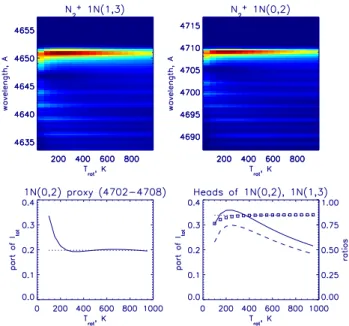
Fig. 4. Top: rotational structure of 1N(1,3) and 1N(0,2) bands,
syn-thetic spectra are convolved with the instrument function for various rotational temperatures of the parent N2. Bottom left – the bright-ness of Proxy(0,2) relative to the total N+2 1N(0,2) band brightness as a function of the rotational temperature. Bottom right – bright-nesses of the Head(0,2) (solid line) and Head(1,3) (dashed line) rel-ative to the total brightness of the respective band, as a function of the rotational temperature. Squares show the ratio of the dashed curve to the solid (axis on the right).
the background BG471, the head of the band Head(0,2) and a broader interval around the band origin Proxy(0,2).
The spectra of the N+2 depend on the rotational temper-ature of the parent N2. To estimate the contribution of the emissions to the selected brightness intervals, synthetic spec-tra for a range of rotation temperatures were convolved with the instrument function. The upper panels in Fig. 4 present rotational development of N+2 1N(0,2) and N+2 1N(1,3) as a function of rotational temperature. The heads of the bands are the most prominent features of the spectra, and those least dependent on the background. However, the portion of the total band brightness contained in its head decreases with in-creasing rotational temperature (see lower right panel).
With the chosen definition of the band head intervals (see Fig. 3), their ratio is independent of the rotational tempera-ture, above 200 K, and is 0.84 (marked with a dotted hori-zontal line in Fig. 4). This means that the ratio of the band brightnesses can be calculated from the ratio of Head(1,3) and Head(0,2), when accounting for this factor. It is possible to choose a spectral interval in such a way that its brightness is proportional to the total brightness of the band within a range of temperatures. The brightness of the Proxy(0,2) in-terval chosen, as shown in Fig. 3, is 0.198 of the total bright-ness of N+2 1N(0,2). This relation holds to within 3% for tem-peratures over 250 K (see lower left panel). This allows one to estimate the total brightness of the N+2 1N(0,2) band from Proxy(0,2). The Head(1,3) is contaminated by the 4650.8 ˚A
Fig. 5. Relative contribution of N+2 1N(1,3) intensity contributing to the O1 (dashes), O2 (dots), and O3 (solid) spectral intervals, vs. the rotational temperature.
O+line. A careful examination of the O+spectra convolved with the instrument function shows that 3.1% of the total O+ multiplet brightness adds to the Head(1,3) brightness, which is subtracted easily.
In the same way, the relative contribution of N+2 1N(1,3) to the interval used for deriving the O+line brightnesses may be estimated. Figure 5 shows these relative contributions as a function of the rotational temperature. The average values of 0.020, 0.035, and 0.055 were used for subtraction from the O1, O2, and O3 brightnesses, respectively. Also, we calcu-late the relative contribution of the O+multiplet to the O1, O2, and O3 brightnesses. Assuming the relative brightnesses of individual lines, as given in Table 1, and convolving those with the instrument function, the relative contributions of the total brightness are 0.057, 0.0207 and 0.357 for O1, O2, and O3, respectively (some of the line brightness “leaks” outside the intervals). In Sect. 3 we confirm that the relative intensi-ties of the oxygen lines are not inconsistent with the assump-tion. However, the O3 spectral interval contains the strongest multiplet line, and least contamination from other (weaker) oxygen and nitrogen lines, and is the best candidate for esti-mating the intensity of the multiplet as the whole.
The background brightness, as estimated from BG465, is often higher than that estimated from the BG486 and BG471, with the two latter brightnesses agreeing very well between themselves (assuming a constant spectral brightness). This is due to the presence of additional unresolved emissions between 4650 ˚A and 4700 ˚A. These emissions have been at-tributed to the N2 2P(0,5) and N2 2P(4,10) bands, as well as the N2 VK(4,16) band (Sivjee, 1980). From our obser-vations, the intensity of these emissions seems to be only weakly related to the presence of the aurora, and they some-times dominate the spectrum when little N+2 1N(0,2) and N+2 1N(1,3) are present. The spectrum from one such occasion,
Fig. 6. Night-sky spectrum devoid of aurora on 13 November 2001, showing the background emissions in the N+2 1N(0,2) and N+2 1N(1,3) panels.
on 13 November 2001, is shown in Fig. 6. Assuming the flat continuum over the whole interval region, the spectral shape can be used to subtract the contribution of these emissions from both N+2 1N(0,2) and N+2 1N(1,3) panels. The intensi-ties of these contaminating emissions are estimated from the difference between BG465 and BG471.
3 Statistical relations between brightnesses
During two intervals (17 December 2001, 12:30–16:30 UT, and 14 January 2002, 18:30–20:30 UT) the intensity of Doppler shifted Hβ emission was well below the intensity
of the unshifted line, indicating that the aurora was excited by electron precipitation. These intervals are studied to es-tablish a statistical relation between the N+2 and O+emission brightnesses.
Figure 7 presents a scatter plot of the brightnesses of the O+multiplet (derived from the O3 brightness, characteriz-ing the strongest line of the multiplet) vs. the intensity of the N+2 1N(0,2) band (further denoted I(0,2)) derived from the Proxy(0,2). There is considerable scatter in the plot, with the linear fit yielding I(O+)=3.1 R + 0.091 I(0,2), with a
correla-tion coefficient of 0.65 for I(0,2) brightnesses below 400 R, and I(O+)=12.0 R+0.064 I(0,2) with a correlation coefficient
of 0.73 for I(0,2)>400 R. The fact that the ratio of the O+ multiplet to the N+2 1N(0,2) decreases with auroral bright-ness is probably due to the fact that there is a correlation between the characteristic energy and the total energy flux in the precipitating electrons (Christensen et al., 1987), brighter aurora being on average produced by more energetic elec-trons.
A useful diagnostic of the data is to look at the rela-tion between the intensities of N+2 1N(0,2) and N+2 1N(1,3) bands. Theory predicts that for parent N2temperatures typi-cal for the ionosphere, the distribution of N+2 ions produced in electron collisions is given by the Franck-Condon fac-tors for the ground vibrational state of the N2 molecule, and the relative intensities of the bands originating from the same upper vibration state are determined by appropriate
Fig. 7. Plot of I(O+) vs. N+2 1N(0,2) in electron aurora. The bright-nesses are derived as I(O+)=O3/0.357 and I(0,2)=Proxy(0,2)/0.198. Red triangles – 17 December 2001 points, cyan diamonds – 14 Jan-uary 2002 points. Solid lines show two linear fits to the data: blue for intensities of N+2 1N(0,2) between 100 R and 400 R, orange – for intensities above 400 R.
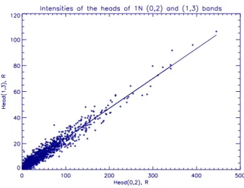
Fig. 8. Plot of Head(1,3) vs. Head(0,2) in electron aurora.
Einstein coefficients. Based on these calculations, the ratio of I(1,3)/I(0,2) should be 0.222. A scatter plot of the Head(1,3) vs. the intensity of the Head(0,2) is shown in Fig. 8. The linear fit to the data is Head(1,3)=1.24 R+0.23 Head(0,2), with a correlation coefficient of 0.967. Taking into consid-eration that the two heads as defined here contain different portions of the band brightnesses (see Fig. 4), and neglect-ing the offset, the ratio of the total band intensities becomes I(1,3)/I(0,2)=(Head(1,3)/0.84)/Head(0,2)=0.27. Though this is 20% higher than predicted by theory, this may be considered a good agreement. There are several possible sources of the discrepancy: the experimental errors, in-cluding the calibration and background subtraction, addi-tional emissions in the spectral interval used for estimating Head(1,3), non-thermal vibrational excitation of the parent
Fig. 9. Plots of O1 vs. O3 (cyan diamonds), and O2 vs. O3 (orange
triangles) in electron aurora. Solid lines show linear fits to the data.
N2, and finally, the deviation of the vibrational development from the Franck-Condon factors.
The relative intensities of the oxygen lines are also in rea-sonable agreement with our assumption of equal probability of the upper sublevel population. Figure 9 shows the scatter plots of O1 and O2 brigtnesses vs. O3. The linear fits yield O1=0.35 R+0.30 O3 and O2=0.04 R+0.42 O3 with corre-lations of 0.66 and 0.70, respectively. The expected values from convolving lines with the instrument function and inte-grating over the intervals used for these lines, are 0.17 and 0.56, respectively (see Sect. 2.3). The O1 brightness is al-most twice the expected value, which is probably due to con-tamination of the spectral interval by other oxygen and nitro-gen emissions. The O2 brightness is 25% below the expected value which is acceptable, taking into account the noise level. 3.1 14 January 2002 event
On 14 January 2002 the spectrograph was operated in 30-s integration mode between 18:30 UT and 20:30 UT. The ESR was running the TAU0 modulation experiment, which uti-lizes two alternating code signals, allowing for complete cov-erage from the E-layer to topside at a time resolution of 6.4 s. The 42-m dish is fixed and aligned in the magnetic zenith, as are the SIF instruments. To improve the signal-to-noise ra-tio and facilitate the comparisons, 32-s time integrara-tion was applied to the radar data prior to the analysis. An aurora of moderate intensity developed in the field of view of the SIF and ESR, allowing for a detailed study of the oxygen emis-sion and its relationship to local ionisation.
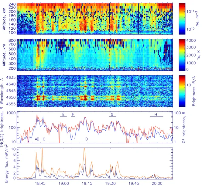
Figure 10 presents an overview of the event. The ESR ob-served enhancements of the E-layer electron number density (top panel), indicative of auroral precipitation – at 18:43 UT, 18:46 UT, 18:53 UT, a weaker one between 18:57 UT and 19:07 UT, at 19:12 UT, 19:14 UT and 19:18 UT, 19:28 UT to 19:36 UT, and around 20:00 UT. These were accompanied by the brightenings of N+2 and O+ emissions (third and
Fig. 10. The event of 14 January 2002. Panels from top to bottom: ESR measurement of electron number density in the E-layer, and electron
temperature in the F-layer; time evolution of 1N(1,3) spectra recorded by the HiTIES; line plots of N+2 1N(0,2) (blue) and O+multiplet (red) intensities; precipitating electron energy flux derived from the radar measurements (blue) and from the optical data (orange). See text.
fourth panels), showing a one-to-one correspondence. In the bottom panel, the energy flux of the precipitating electrons derived from the ESR ionization profiles (see below) is compared with the energy flux determined from N+2 1N(0,2) emission (using a conversion factor of 45 R per 1 mW/m2, derived from our model – see below). Even though the instruments are 7 km apart, which means that the magnetic zenith of the SIF does not coincide with that of the ESR, the qualitative agreement of the curves warrants the further consideration of the data. For integration times of 30 s, as used here, fast motions of the aurora in most cases provide the spatial averaging to make the comparison valid.
The brightnesses of the oxygen ion multiplet, and the nitrogen first negative emissions follow each other rather closely when the latter are scaled with the factor of 0.1, as
found above (note the different scale for the O+ brightness in panel 4). However, a closer look at the data reveals several regions where the proportionality is not observed. Between 18:35 UT and 18:48 UT the O+lines are relatively stronger (apart from one point at 18:47 UT where strong N+2 1N(0,2) is observed), as they are between 19:04 UT and 19:08 UT, and 19:47 UT to 20:10 UT. Several representative intervals were selected for joint analysis of the data. Where aurora is sufficiently intense (intervals A, B, C, and D) single integra-tion periods of the spectrograph and radar data are put in the context of the imager data. For intervals E, F, G and H the precipitation was less intense, rendering the imager data less useful. For these intervals several electron number density profiles and HiTIES spectra had to be integrated. The results of the analysis of all these intervals, as described in detail below, are summarized in Table 2.
Table 2. Summary of the intervals on 14 January 2002: characteristic energy of the best fits for maxwellian and monoenergetic input
electron spectra, quality of the fit, observed ratio of O+4P-4D0multiplet intensity to the N+2 1N(0,2) intensity, modeled brightness from the O2dissociative ionisation/excitation, difference between the observed O+brightness and O2+econtribution, modeled brightness from O+e assuming maximum cross section of 0.18×10⁻¹⁸cm2.
A B C D E F G H
Emaxw, keV 0.50 0.97 0.80 0.88 0.50 0.50 0.73 0.50
Emono, keV 1.07 2.78 2.53 3.06 1.90 1.07 2.30 1.07
Fit fair fair fair good poor fair good poor I(O+)/1N(0,2), ×100 14.62 17.32 6.90 10.23 12.55 12.61 12.6 22.54 Imod(O2→O+)/1N(0,2), ×100 1.92 2.42 2.34 1.92 2.17
I(O→O+)/1N(0,2), ×100 12.7 14.9 7.89 10.7 10.43 Imod(O→O+)/1N(0,2), ×100 11.4 7.9 8.2 11.4 9.2
Fig. 11. Snapshots of four intervals on 14 January 2002. For each of the intervals two images from the SIF narrow field imager are given,
the ESR electron number density altitude profile, and the HiTIES spectrum of the N+2 1N(1,3) wavelength interval. Solid lines in the density profiles show a fit with the maxwellian precipitation, and dashed lines – monoenergetic precipitation. See text.
the energy flux and characteristic energy of the precipitation. This simple and relatively coarse method has been shown to produce reliable results (Lanchester et al., 1998). The fit for the energy flux will be an underestimate in time-varying au-rora for two reasons. The integration of the radar spectra over a time interval is linear in density (which is given by the power of the scatter in the first approximation), whereas the energy flux is given by the square of the equilibrium density. Also, the assumption of ionisation-recombination equilibrium itself breaks down at short time-scales compared with the recombination time scale, which varies between un-der a second below 100 km and tens of seconds in the upper E-layer and lower F-layer. The fitted value for the character-istic energy, on the other hand, depends mostly on the shape of the profiles, and thus is less affected by the time variations in the characteristic energy of the precipitation.
Figure 11 presents data from single ESR and SIF mea-surements, together with representative camera images from within the integration periods. Interval A, centred around 18:42:00 UT, is in the beginning of a period of bright au-rora in the field of view of the SIF. The activity starts as a rayed arc comes from the south (top of the camera images) at around 18:41:30 UT. Rays and structured rayed arcs appear throughout the field of view, moving and changing inten-sity rapidly. During this interval the radar recorded densities ranging between 1×10¹⁰m−3 and 4×10¹⁰m−3at altitudes between 100 km and 180 km. The best fits have characteristic energies of 1.07 keV (monoenergetic electrons) and 0.5 keV (maxwellian distribution) respectively. Both fits predict more pronounced peaks of the ionisation than those observed, with maxwellian precipitation being probably closer to reality. In the N+2 1N(1,3) panel the oxygen line at 4649.13 ˚A is the brightest feature (when considering spectral brightness).
The next sample of both instruments is selected as in-terval B. The rays intensify, and are observed as coronal structure as they fill the entire field of view of the cam-era. In the magnetic zenith a very narrow structure trans-verse to the magnetic field is present. The ESR electron densities are now over 1×10¹¹m−3for most of the altitude range between 100 km and 180 km. As in the previous inter-val, the fall-off of the electron density with altitude is rather slow, even though there is a more pronounced peak at about 115 km. The maxwellian fit with the characteristic energy of 0.97 keV is again closer to the data than the monoenergetic with 2.78 keV energy, both falling short of the measured elec-tron concentrations above 150 km. The N+2 1N(1,3) panel spectrum shows strong oxygen lines, at higher intensities.
measurements, they cannot be directly compared to the Hi-TIES spectrum, which shows a dominating peak of the N+2 1N(1,3) band.
Interval D is chosen as a brightest point within the auroral event observed between 19:10 UT and 19:20 UT. Through-out the event the intensities of the O+ lines and the N+
2 1N(0,2) are related by the factor of 0.1. The imager ob-served “diffuse” aurora covering much of the field of view, with dark structures appearing inside it. The appearance of the aurora is clearly distinctive from the rays characteristic of intervals A and B. The ionisation profile produced by the maxwellian distribution of electrons with characteristic en-ergy of 0.88 keV is in good agreement with the observed density profile, while the monoenergetic (3.06 keV) profile underestimates the density both below and above the peak, which itself is reproduced somewhat better.
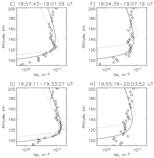
Figure 12 shows the ESR density profiles for intervals E, F, G, and H, together with the monoenergetic and maxwellian ionisation profiles. In cases F and H the O+lines are well
above the average of 0.1 of the N+2 1N(0,2) brightness, and the both density profiles lack a clear E-region peak. The mo-noenergetic profiles fail to reproduce the density distribution, while the maxwellian ones are closer to the observation, but still predict an ionisation peak between 120 and 140 km. Pro-file E (with a ratio of O+ multiplet to N+2 1N(0,2) bright-ness close to 0.1) shows both a peak at just above 120 km, and a flat profile above the peak, which results in a rather poor fit for both the maxwellian and the monoenergetic dis-tributions. Finally, case G corresponds to an interval where the O+ lines are only slightly above the average 0.1 of the N+2 1N(0,2) intensity, and the ionisation profiles corresponds well to a maxwellian precipitation with characteristic energy of 0.73 keV.
The second panel in Fig. 10 shows the F-layer electron temperature. There are several enhancements of the electron temperature, the most pronounced one being related to the in-terval 18:40 UT to 18:50 UT, when rayed arcs were observed (intervals A, B and C). In contrast to this, interval D does not show any significant enhancements in Te, even though the
electron concentration produced in the E-layer is even higher than for the former intervals.
3.2 Estimation of the excitation cross sections
To study the excitation of the 4P-4D0 multiplet we use an electron transport model, together with a model cross section energy dependence. By comparing the predicted
Fig. 12. ESR density profiles and SIF spectra for intervals E, F, G and H in Fig. 10.
I(O+)/I (0, 2) ratios for maxwellian input spectra with char-acteristic energies obtained from the fits (see Table 2) to ob-served ratios, the absolute scale can be put on the cross sec-tion.
The excitation energy of the O+4D0state is 25.66 eV. The abundance of ionized oxygen is several orders of magnitude below that of the neutrals in the altitude range where the au-roral emissions can be produced (80–500 km), so excitation of O+will make a negligible contribution to the production of the multiplet. Thus, the viable processes for production of the lines are the ionization-excitation with the threshold of 39.27 eV:
O + e → O+(4D0) + esec+e, (1)
and the dissociative ionization of O2 with the threshold of 44.39 eV
O2+e →O+(4D0) +O + esec+e. (2)
To the best of our knowledge, no measurements or theo-retical calculations provide the differential cross section for reaction (1). For the allowed transitions the electron impact excitation cross sections behave asymptotically at high en-ergies as E−1ln E, exhibiting a maximum at 4–5 threshold
energies (Vallance Jones, 1974). We assume a model cross section in the functional form of
σ (E) ∝ (1 − e−0.3E−E0E0 )E−1ln E, (3) corresponding to maximum cross section at 160 eV (see Fig. 13).
The cross section for reaction (2) has been measured by Schulman et al. (1985) as a by-product of their work on the neutral oxygen atom emissions produced in electron impact dissociative ionization of O2. It was found that the cross sec-tion for the two 3s4P1/2,5/2−3p4D01/2,7/2lines at 4650 ˚A has a maximum at 200 eV, where its value is 0.17×10⁻¹⁸cm2. These two lines amount to 0.484 of the total brightness of the multiplet.
The above cross sections were used, together with an elec-tron transport model for the ionosphere (Lummerzheim and Lilensten, 1994), to estimate the brightnesses of the produced emissions. To obtain a quantitative scale on the cross section, a series of model runs was made for the cases where the best fit to the electron density profiles was achieved (cases A, B, D, F and G). Maxwellian distributions with corresponding characteristic energies were used as input at 500 km with a 1 mW/m2 energy flux. The model calculated the mag-netic zenith brightness of the N+2 1N(0,2) band, assuming the
Fig. 13. Model shape of the cross section for production of the
O+4D0state from atomic oxygen.
branching ratio of 0.145 for production of N+2(B) state (van Zyl and Pendleton, 1995), and using the value of 0.04 for the ratio of N+2 1N(0,2) to the total first negative system intensity (Vallance Jones, 1974). Also, the brightness of the O+ multi-plet produced in (2) was calculated, and that directly excited in (1). The ratios of the O+brightnesses were compared to the observed ratio in the selected cases. Comparing the ob-served brightnesses with the predicted ones indicates that the excitation in the dissociative ionisation contributes to a small portion of the total multiplet brightness (see the fourth row in Table 2), the bulk of the emissions coming from the direct process. The second row from the bottom in Table 2 shows the observed value of the brightness produced in the direct O+e processes, which was obtained as the difference of the observed I(O+)/I (0, 2) and the modelled contribution from O2dissociative ionization. Scaling the model cross section shape to the maximum value of 0.18×10⁻¹⁸ cm2 results in the best fit between the modelled (last row) and the observed value of the brightness excited in the ionisation of atomic O. Using this cross section, the energy dependence of the O+
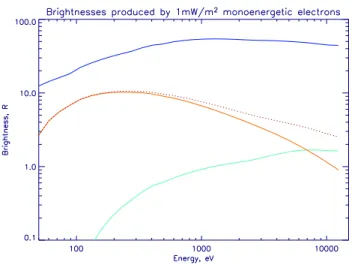
line emission rate was studied. A number of runs were made for monoenergetic electrons with the energy flux at 500 km of 1 mW/m2. Figure 14 shows the calculated height-integrated emission rates of the O+multiplet produced in the ionization excitation of O, due to dissociative ionization of molecular oxygen, as well as the N+2 1N(0,2). The oxygen multiplet is most sensitive to the low energy precipitation, producing maximum brightness at 200 eV. At low energies the dissocia-tive ionisation is negligible, but becomes comparable to the direct ionisation of atomic oxygen at energies of about 7 keV.
4 Discussion
The 14 January 2002 event contained several instances of electron precipitation with varying characteristics in the field of view of the instruments. The ratio of the intensities of the
Fig. 14. Height-integrated emission rate of N+2 1N(0,2) band (blue curve) and O+multiplet vs. the energy of monoenergetic electron precipitation. Green curve shows the intensity due to the dissocia-tive ionisation, red curve shows the intensity due to the direct ion-isation of O (using the cross section estimated in this work). The dotted line is the total O+multiplet intensity.
O+multiplet to the N+
2 band emission appears to be strongly related to the type of auroral forms in the field of view of the optical instruments, which is borne out by the variable height profiles of electron concentration measured by the radar, and by the occurrence of raised electron temperatures in struc-tured rayed aurora. We have used these differences to in-vestigate the mechanisms for production of the O+ multiplet and to estimate the cross section for one of the production mechanisms.
The intensity ratio of the N+2 1N(1,3) and N+2 1N(0,2) bands is somewhat larger than that predicted from Franck-Condon factors. Also, the brightness of the 4638.9 ˚A and 4641.8 ˚A lines relative to the 4649.1 ˚A line are somewhat different than those assuming equal probability excitation of the states. In both cases the discrepancies can proba-bly be accounted for by the measurement errors and other contaminating emissions, which become more important for relatively weaker spectral features. Quite noticeable is the difference between the energy flux derived from the radar ionisation profiles, and the N+2 1N(0,2) brightness. The en-ergy flux derived from the first negative band brightness ex-ceeds that from the radar measurements by a factor of 2 to 3. This is the case even though the atmospheric extinc-tion of the emission has not been taken into account. This could have decreased the observed intensities by a factor of 1.5 (Lummerzheim et al., 1990). A similar discrepancy was noted by Vallance Jones et al. (1987), who attributed it to the cumulative result of small errors in calibrations, recombination coefficient used and cross sections employed in the model. Another possibility, which should be pointed out, is that the nature of the time and space integration is dif-ferent for optical and radar measurements. Whereas the op-tical emissions intensity is proportional to the energy flux of
the precipitation, the equilibrium ionospheric density is pro-portional to the square root of the energy flux. So, unless the precipitation is constant in time for the whole integration pe-riod and in space across the whole field of view of the radar, the radar estimate will be an underestimate of the energy flux. The situation is similar to that discussed by Semeter and Doe (2002) encountered in interpreting the ionospheric conduc-tance derived from global auroral images.
The observed enhancement of the O+ lines is associated with ionisation in the upper E-layer. In most of the analyzed profiles from the 14 January 2001 event, the Maxwellian precipitating electron spectra fitted the data better than the monoenergetic beam. This is not the case generally, and Strickland et al. (1994) present examples of both types of profiles. They attribute the maxwellian spectra to the dif-fuse aurora. In our case, the intervals A and B are associ-ated with the highly structured rayed arcs and enhanced elec-tron temperature in the topside F-layer. Such arcs, observed as coronal structures in the images, are reported to be as-sociated with coherent radar spectra (Sedgemore-Schulthess et al., 1999), which are often interpreted in terms of cur-rent instabilities. High field-aligned curcur-rent densities were reported by Lanchester et al. (2001) from analysis of highly enhanced electron temperature in a structured aurora, and by satellite measurements (e.g. Ivchenko and Marklund, 2002). Such high current densities are most probably transient and are related to Alfv´enic structures associated with the aurora (Stasiewicz et al., 2000). Dispersive Alfv´en waves are related to suprathermal electron bursts – field-aligned population ex-tending up to 1 keV energies (e.g. Andersson et al., 2002). Such precipitation should be effective in exciting F-region auroras (Chaston et al., 2003).
A major uncertainty in the derivation of the emission cross section by comparison of the model with the observations lies in the altitude profiles of the neutral constituents. Partic-ularly, the concentration of atomic oxygen at high latitudes may differ from the MSIS90 model (used in the electron transport code) by a factor of up to 2 (Lummerzheim et al., 1990; Shepherd et al., 1995; Nicholas et al., 1997), which is attributed to the effects of the aurora itself (Christensen et al., 1997).
Few studies have been made into the cross sections of O+ emissions, which could be related to auroral and air-glow studies. Apart from the cited paper by Schulman et al. (1985) mentioning the cross section of the 4P-4D0 multiplet, the only other paper we are aware of is that by Haasz and deLeeuw (1976). They measured effective emis-sions cross sections of O+ lines at 4350 ˚A and 4416 ˚A.
For the excitation of these two multiplets from the elec-tron collisions with neutral oxygen atoms, the values of 2.3×10⁻²⁰cm2and 5.9×10⁻²⁰cm2, respectively, were ob-tained; for the dissociative ionisation-excitation of O2, the values were 1.45×10⁻²⁰cm2and 1.40×10⁻²⁰cm2, respec-tively. However, their cross sections were obtained for the energy range of 0.6 to 3.0 keV, and thus cannot be directly compared to our result. It should also be pointed out that our results, as well as those by Haasz and deLeeuw (1976) and
Schulman et al. (1985), refer to emission cross sections, in-cluding cascading from higher lying states, possibly excited by electron impact.
5 Conclusions
1. The4P-4D0multiplet of ionized oxygen is persistently present in the electron aurora. Its intensity amounts, on average, to 0.1 of N+2 1N(0,2) intensity.
2. The O+lines are relatively brighter in low characteris-tic energy electron precipitation, which is in agreement with electron transport model calculations.
3. Comparison of the observations with a model shape of the differential cross section yields a peak cross section of 0.18×10⁻¹⁸cm2 for the assumed functional form of the energy dependence. The main source of uncer-tainty is associated with using the MSIS90 atomic oxy-gen concentrations, which may disagree with the actual concentrations in the auroral zone.
4. Rayed arcs are observed to be associated with en-hanced O+line brightnesses, and E-layer density pro-files that decrease slowly with altitude. Also, enhanced F-layer electron temperature is associated with the in-terval when the rayed arcs are observed.
5. The observed ratios between the brightnesses of N+2 1N(1,3) and N+2 1N(0,2) bands are about 20% higher than those predicted by the Franck-Condon fac-tors, which should not be taken as a discrepancy, consid-ering that various theoretical predictions differ between themselves.
Acknowledgements. NI is supported by a grant from PPARC in the
UK. MG is supported by NASA grant NAG5-12773. The EIS-CAT Scientific Association is supported by Centre National de la Recherche Scientifique of France, Max-Planck-Gesellschaft of Ger-many, Particle Physics and Astronomy Research Council of the United Kingdom, Norges Forskningsr˚ad of Norway, Naturveten-skapliga Forsknings˚adet of Sweden, Suomen Akatemia of Finland and the National Institute of Polar Research of Japan.
Topical Editor M. Lester thanks C. Deehr and K. Kaila for their help in evaluating this paper.
References
Andersson, L., Ivchenko, N., Clemmons, J., Namgaladze, A. A., Gustavsson, B., Wahlund, J.-E., Eliasson, L., and Yurik, R. Y.: Electron signatures and Alfv´en waves, J. Geophys. Res., 107, 15–1, 2002.
Chakrabarti, S., Pallamraju, D., Baumgardner, J., and Vaillancourt, J.: HiTIES: A high throughput imaging echelle spectrograph for ground-based visible airglow and auroral studies, J. Geophys. Res., 106, 30 337–30 348, 2001.
Chamberlain, J. W.: Physics of the Aurora and Airglow, Academic Press, New York and London, 1961.
Degen, V.: Modeling of N2/+/ first negative spectra excited by elec-tron impact on N2, J. of Quant. Spectr. and Rad. Trans., 18, 113– 119, 1977.
Fordham, J. L., Bellis, J. G., Bone, D. A., and Norton, T. J.: MIC photon counting detector, in: Proc. SPIE, Vol. 1449, Electron Image Tubes and Image Intensifiers II, edited by Csorba, I. P., 87–98, 1991.
Haasz, A. A. and deLeeuw, J. H.: Effective electron impact exci-tation cross sections for N2, O2, and O1, J. Geophys. Res., 81, 4031–4034, 1976.
Ivchenko, N. and Marklund, G.: “Current singularities” observed on Astrid-2, Adv. Space Rec., 30, 1779–1782, 2002.
Ivchenko, N., Galand, M., Lanchester, B. S., Rees, M. H., Lum-merzheim, D., Furniss, I., and Fordham, J.: Observations of O+ (4P-4D0) lines in proton aurora over Svalbard, Geophys. Res. Lett., doi:10.1029/2003GL019313, 31, 2004.
Kerr, R. B., Garcia, R., He, X., Noto, J., Lancaster, R. S., Tepley, C. A., Gonz´alez, S. A., Friedman, J., Doe, R. A., Lappen, M., and McCormack, B.: Periodic variations of geocoronal Balmer-alpha brightness due to solar-driven exospheric abundance variations, J. Geophys. Res., 106, 28 797–28 818, 2001.
Lanchester, B. S., Rees, M. H., Sedgemore, K. J. F., Palmer, J. R., Frey, H. U., and Kaila, K. U.: Ionospheric response to variable electric fields in small-scale auroral structures, Ann. Geophys., 16, 1343–1354, 1998.
Lanchester, B. S., Rees, M. H., Lummerzheim, D., Otto, A., Sedgemore-Schulthess, K. J. F., Zhu, H., and McCrea, I. W.: Ohmic heating as evidence for strong field-aligned currents in filamentary aurora, J. Geophys. Res., 106, 1785–1794, 2001. Lanchester, B. S., Rees, M. H., Robertson, S. C., Lummerzheim, D.,
Galand, M., Mendillo, M., Baumgardner, J., Furniss, I., and Ayl-ward, A. D.: Proton and electron precipitation over Svalbard – first results from a new Imaging Spectrograph (HiTIES), Proc. of Atmospheric Studies by Optical Methods, Sodankyl¨a Geophys. Obs. Pub. 92, 33–36, 2003.
Lummerzheim, D.: Electron Transport and Optical Emissions in the Aurora., Ph.D. Thesis, 1987.
Lummerzheim, D. and Lilensten, J.: Electron transport and energy degradation in the ionosphere: Evaluation of the numerical solu-tion, comparison with laboratory experiments and auroral obser-vations, Ann. Geophys., 12, 1039–1051, 1994.
Lummerzheim, D., Rees, M. H., and Romick, G. J.: The application of spectroscopic studies of the aurora to thermospheric neutral composition, Planet. Space Sci., 38, 67–78, 1990.
McWhirter, I., Furniss, I., Lanchester, B. S., Robertson, S. C., Baumgardner, J., and Mendillo, M.: A new spectrograph plat-form for auroral studies in Svalbard, Proc. of Atmospheric Stud-ies by Optical Methods, Sodankyl¨a Geophys. Obs. Pub. 92, 73– 76, 2003.
cance of resonant scatter in the measurement of N2 first negative 0-1 emissions during auroral activity, J. Atmos. Terr. Phys., 63, 295–308, 2001.
Schulman, M. B., Sharpton, F. A., Chung, S., Lin, C. C., and Anderson, L. W.: Emission from oxygen atoms produced by electron-impact dissociative excitation of oxygen molecules, Phys. Rev. A, 32, 2100–2116, 1985.
Sedgemore-Schulthess, K. J. F., Lockwood, M., Trondsen, T. S., Lanchester, B. S., Rees, M. H., Lorentzen, D. A., and Moen, J.: Coherent EISCAT Svalbard Radar spectra from the dayside cusp/cleft and their implications for transient field-aligned cur-rents, J. Geophys. Res., 104, 24 613–24 624, 1999.
Semeter, J. and Doe, R.: On the proper interpretation of ionospheric conductance estimated through satellite photometry, J. Geophys. Res., pp. 19–1, 2002.
Semeter, J., Lummerzheim, D., and Haerendel, G.: Simultaneous multispectral imaging of the discrete aurora, J. Atmos. Solar-Terr. Phys., 63, 1981–1992, 2001.
Shepherd, M. G., McConnell, J. C., Tobiska, W. K., Gladstone, G. R., Chakrabarti, S., and Schmidtke, G.: Inference of atomic oxygen concentration from remote sensing of optical aurora, J. Geophys. Res., 100, 17 415–17 428, 1995.
Sivjee, G. G.: Anomalous vibrational distribution of N2/+/1 NG emissions from a proton aurora, J. Geophys. Res., 85, 206–212, 1980.
Stasiewicz, K., Bellan, P., Chaston, C., Kletzing, C., Lysak, R., Maggs, J., Pokhotelov, O., Seyler, C., Shukla, P., Stenflo, L., Streltsov, A., and Wahlund, J.-E.: Small Scale Alfv´enic Struc-ture in the Aurora, Space Sci. Rev., 92, 423–533, 2000. Strickland, D. J., Hecht, J. H., Christensen, A. B., and Kelly, J.:
Re-lationship between energy flux Q and mean energy (mean value of E) of auroral electron spectra based on radar data from the 1987 CEDAR Campaign at Sondre Stromfjord, Greenland, J. Geophys. Res., 99, 19 467–19 473, 1994.
Vallance Jones, A.: Aurora, D. Reidel Publishing Company, Dor-drecht, Holland, 1974.
Vallance Jones, A., Gattinger, R. L., Shih, P., Meriwether, J. W., and Wickwar, V. B.: Optical and radar characterization of a short-lived auroral event at high latitude, J. Geophys. Res., 92, 4575– 4589, 1987.
van Zyl, B. and Pendleton, W.: N+2(X), N+2(A), and N+2(B) produc-tion in e−+N2collisions, J. Geophys. Res., 100, 23 755–23 762, 1995.
Wannberg, G., Wolf, I., Vanhainen, L.-G., Koskenniemi, K., R¨ottger, J., Postila, M., Markkanen, J., Jacobsen, R., Stenberg, A., Larsen, R., Eliassen, S., Heck, S., and Huuskonen, A.: The EISCAT Svalbard radar: A case study in modern incoherent scat-ter radar system design, Radio Science, 32, 2283–2307, 1997.