Dynamic And Static Green's Functions In Transversely Isotropic Elastic Media

IN TRANSVERSELY ISOTROPIC ELASTIC MEDIA

by

Wenjie Dong

Earth Resources Laboratory

Department of Earth, Atmospheric, and Planetary Sciences Massachusetts Institute of Technology

Cambridge, MA 02139

and

Denis P. Schmitt

Mobil Exploration and Producing Technical Center 3000 Pegasus Park Drive

Dallas, Texas 75247

ABSTRACT

Concise and numerically feasible dynamic and static Green's functions are obtained in dyadic form by solving the wave equation and the equilibrium equation with general source distribution in transversely isotropic (TI) media. The wave and equilibrium equations are solved by using an extended version of the Kupradze method originally developed for isotropic media. The dynamic Green's function is expressed through three scalar quantities characterizing the propagation ofSH and P-SV waves in a transversely isotropic medium. The 2-D inverse Laplacian operator contained in previous Green's function expressions is eliminated without limiting to special cases and geometries. The final dyadic form is similar to that of the isotropic dyadic Green's function, and therefore lends itself to easy analytical and numerical manipulations. The static Green's function has the same dyadic form as the dynamic function except that the three scalars must be redefined. From the dynamic Green's function, displacements due to vertical, horizontal, and explosive sources are explicitly given. The displacements of the explosive source show that an explosive source in a TI medium excites not only thequasi-P wave, but also the quasi-SV wave. The singular properties of the Green's functions are also addressed through their surface integrals in the limit of coinciding receiver and source. The singular contribution is shown to be -1/2 when the static stress Green's function is integrated over a half elliptical surface.

INTRODUCTION

Wave propagation from various seismic sources placed inside a fiuid-filled borehole em-bedded in a layered transversely isotropic medium is of great interest and importance to geophysicists dealing with crosshole, vertical seismic profiling, and acoustic logging data. In simulating wave propagation in this geometry, ordinary numerical techniques, such as the finite difference method and the finite element method, encounter computational difficulties because of the significant scale difference between the borehole diameter and the formation extent. A technique (Bouchon, 1992; Dong et a!., 1992) perfectly suited to this kind of geometry is the boundary element method (BEM). It is a semi-analytical method because the only discretization occurs at the borehole boundary and the prop-agation of waves is realized through the use of the dynamic Green's function. This technique also requires the static Green's function to regularize the boundary surface integral when the source and the receiver coincide. These essential requirements of the Green's functions in the BEM technique motivate this work.

Although plane wave propagation in TI media has been studied by many workers (e.g. Fedorov, 1968; Crampin, 1985; among others), literature on the static and dynam-ic Green's functions of the TI medium are at most scarce. Among the existing ones, most of them provided the solution in component and numerical forms. Pan and Chou (1976) presented explicit solutions of the equilibrium equation in terms of displacement and stress components for vertical and horizontal forces. In their solution procedure, three displacement potentials and an assumed solution form with unknown coefficients were used. Buchwald (1959) solved the wave equation for three strains:

(~- ~

),

8;;

and (~+ ~

).

The far-field approximation of these strains was given using a stationary phase approximation. Other workers (White, 1984; White et a!., 1984; Man-daI and Toksoz, 1990) employed numerical method to study the radiated waveforms of line source, vertical and horizontal point forces, and explosion source. Kazi-Aoual et a!. (1988) devised an algorithm using the Kupradze method (Kupradze, 1979) for calcu-lating the dynamic Green's function. In Kazi-Aoual et a!. (1988), the dynamic Green's function is expressed as the cofactor matrix of a symmetrical matrix of differential op-erators operating on a single scalar. The scalar is represented by the Hankel transform. Ben-Menahem and Sena (1990) and Sena (1992) extended the work of Buchwald and obtained the dynamic Green's tensor in the form of the Hankel transform by recovering the displacement vector from the three strains. This extension is significant because a fairly simple dynamic Green's tensor is given in terms of dyadic notation. However, due to the presence of a 2-D inverse Laplacian operator in the expression, this Green's function does not lend itself easily to numerical and analytical manipulations.

In this paper, we present a unified treatment of the dynamic and the static Green's functions and show that they can be conveniently expressed by a single dyadic form, with different meanings of the symbols for each case, of course. Unlike the previous

= -FXl -Fy , -Fz • (1) -Ft,(2) -Fz,(3)

studies, we solve the equilibrium and wave equations with a general source distribution by using an extended version of the Kupradze method. This not only simplifies the previous derivations but also enhances their rigorousness. More importantly, the final solution does not contain the2-D inverse Laplacian operator and is valid for the source at an arbitrary location, which is critical for the BEM technique. We then apply the dynamic Green's function to obtain the displacements for the vertical, horizontal and explosive point sources. Finally, the static Green's function is used to compute the singular contribution when integrating the dynamic stress function over a boundary surface in the limit of the source coinciding with the receiver. These results are directly applicable to BEM simulation of wave radiation and scattering.

THE DYNAMIC GREEN'S FUNCTION

In a Cartesian coordinate system (x,y,z) with unit vector (x,y,z), let U= _(uz,uy,uz)

and F = _{(Fz , Fy, F}z ), respectively, be the displacement vector and external body force

of a transversely isotropic medium characterized by the five independent elastic stiffness constants, Cn, C13, C33, C44, and C66. The frequency domain wave equation in terms of the displacement components for a transversely isotropic medium can be written in the following form

82uz 82uz 82uz ) 82uy ) &uz 2

cn _8x2 + _{C66 8 y2} + _{C44 8z2} + (Cn - C66 8x8y + (C13 + C44 8x8z + pw Uz

82uy 82uy &uy ) &uz ) 82uz 2

cn 8y2 +C66 8x2 + _{C44 8z2} + (Cn - CS6 8x8y + (C13 + C44 8y8z + pw u y &uz (&uz &uz) ( ) 8 (8Uz 8Uy ) 2 C33 8z2 + C44 8x2 + 8y2 + cI3 + C44 8z 8x + 8y + pw Uz

In the above equation, the relation CI2

=

Cn - 2C66is used. These equations can be easily compared with those in White (1983), where Love's notation for the elastic constants is used. Grouping the first two equations together in terms of transverse displacement, Ut

=

uzx +uyy, and rewriting the third equation, we obtain

2 &Ut 8 2

CS6V't Ut+ C44 _8z2 +(Cl1-CS6)V'tV't·Ut+(CI3+C44)8zV'tUz+PW Ut

2 82uz 8 2

C44V't Uz+ _{C33 8z2} + (C13 + C44) 8zV't· Ut + pw Uz

where, Ft

=

Fzx+ Fy'fj. Similar to solving the elastic wave equation for the isotropic case, where the curl and divergence are taken on both sides of the equation, Eqs. (2) and (3) can be solved by taking the transverse curl and the transverse divergence on both sides.

(4) We first take the transverse curl, defined as \7tx = [\7 -

;'E]

x, of Eq. (2) to obtain

2

&

2

c66\7t \7,

x

Ut +C448z2 \7,

x

U,

+

pw \7t

x

Ut = -\7t

x

F,.

\7t x Ut = lvg(x,x/) \7; x F;

dX,

(5)

where x

==

(x,y,z) is the receiver location, and x'

==

(x',y'ZI) is the source location. g(x,x') is the Green's function of the scalar wave equation

The gradient terms disappeared because \7t X \7,u

=

O. By virtue of Green's

super-position theorem, the solution of this equation in terms of the transverse curl of Ut is

(6) This function is readily obtained following transformation s

=

JC66/C44 Zand 6(az)

=

1/a6(z). If

e-

iw_{' dependence is assumed for the wavefield, this Green's function is}

e ikoR

g(x,x)= 4

y'C44C66R'

1r C44C66 (7)

where, R

=

J(x - xlF

+

(y - yiP

+

Cs6!C44(Z ZI)2 is the distance from the source to the receiver and ko

=

w/J C66/p is the wave number. In the isotropic limit, C66

=

C44

=

11, and 9 reduces to the scalar shear wave Green's function.

Taking the transverse divergence of eq. (2) and the

z

derivative of eq. (3), we obtain two coupled equations,

(8)

(9) These equations can be solved using an extended version of the Kupradze method (Kupradze, 1963) outlined for an isotropic medium. First, we rewrite the coupled equa-tion in a matrix form

where

(11)

In the Kupradze method, the unknowns of the system are expressed in terms of the cofactor matrix of the original symmetrical matrix operating on a single scalar. The system is greatly simplified because the product of a sy=etrical matrix and its cofactor matrix results in an identity matrix scaled by the determinant of the original matrix. This method no longer applies in our case due to the loss of symmetry of the matrix in Eq. (10). Kazi-Aoual et al. (1988) can still apply the Kupradze method because they solve Eq. (1), which is symmetric when written in matrix form. Instead of the cofactor matrix, the adjoint of the original matrix must be used for the nonsy=etrical system. The adjoint of a matrix is defined as the transpose of its cofactor matrix. The product of a matrix with its adjoint is the identity matrix scaled by its determinant. Following this method, we assume

[ 'Vt . lit ]

-1 [

Lt

-(CIS

+

C44)'Vl ] A.( ') [

'V~

.

F~

] d I

au_

-

)a

2 _",X,x

aF

'

x.

fu V -(CI3

+

C44 a;:t Lz Cf?' z

Substituting Eq. (13) into Eq. (10), we obtain

[LtLz - (CIS

+

C44)2

;;2

'V

_F]

¢(x, X') = -6(x - X').

(13)

(14)

(17) The scalar Eq. (14) can be solved using the Fourier transform method. Defining the 3-D spatial Fourier transform as follows,

FT{f(x)}

=

1..:

dz

1..:

dV

1..:

dx!(x)e-i1k,,(x-x')+k,,(y-y')+k.(z-z')I, (15) and applying it to the above equation, we have

¢(kx, ky, k., w)

=

(cllk2

+

_{C44 k; _ pw2)(C44 k2}

+

~~3k;

_ pw2) _ (CIS

+

C44)2Pk;' (16) where, k 2

=

k~

+

k~ is the transverse or horizontal wavenumber. To return to the spatial coordinates, one takes the inverse transform first, then changes the rectangular space (x - x', V - V', z - Zl) and wavenumber _{(kx, ky, kz)} domain into cylindrical coordinates (D, OD, z) and _{(k, Ok, kz).} Integration over Ok produces a zeroth order Bessel function of the first kind, i.e., 21rJo(kD)

=

It"

dOkeikDcos(9k-9D). The final result is

I -1

foco

lco

eik:(z-z')

¢(x, x, w)

=

(2 )2 kJo(kD)dk dkz(P 2)(P 2)'

1r C33C44 0 -co z - Va z - Vb

In this equation, D

=

v'(x XI)2

+

(V - V' )2, and v~ and v~ represent the two roots of the denominator in Eq. (16), corresponding to quasi-P and quasi-SV waves, respec-tively. After regrouping terms, the denominator is

CSSC44k;

+

[(CllCSS - cis - 2CISC44)k2 - (css

+

C44)pw2]k;

whose roots are V~ = where, (C33

+

C44)pw2 - (CnC33 - q3 - 2CI3C44)P

+

v'

Ak4

+

BP

+

C

2CaaC44 ' (C33

+

C44)pw2 - (CnC33 - q3 - 2CI3C44)k2 -

v'

Ak4

+

BP

+

C

V2 = a 2C33C44 A = (CnC33 - CI3)[CnC33 - (CI3

+

2C44?], B - -2pw2(C33 - C44)[CnC33 - (CI3

+

2C44)2], +4pw2C44 (CI3

+

C44)(CI3

+

2C44 - C33) C

=

(C33 - C44)2 p2W4. (19) (20) (21)

To calculate the kz integral properly, one should notice that the integrand has four

poles at k_z = _{±va and} k_z = ±Vb. Moreover, for a real w, these four poles lie on the real kz axis, rendering the integral undefined. However, if a complexw is assumed, these

poles are off the real axis, and the integral is well-defined. If we assume Im[val

>

0 and

1m

[VbJ

>

0, then for

z -

z'

>

0, we have to close the contour in the upper half of the

k_z plane. By Cauchy's theorem, the real axis integration is equivalent to 211" times the residue of poles at kz

=

Va and kz

=

Vb. Similarly, for

z -

Zl

<

0, the integral is equal to the pole contribution at -Va and -Vb. The combined result valid for all

z -

Zl is

- i

10

00

1

(eiV,lz-z'r

eivarz-z'I)

¢(x,x',w) = 4 2 2 - kJo(kD)dk.

7rC33C44 a Vb - va Vb Va (22)

Once9 and ¢ are determined, we obtained the transverse curl, the transverse diver-gence, and the

z

derivative of the displacement vector, u. These quantities are

'Vt x Ut

₌

'Vt · Ut

₌

au

z

=

az

(23) (24) (25) (26)

Now, a few vector identities and integration by parts can be used to recover the total displacement vector. Using vector identity g'Vi xf'

=

'Vi X (gfl) - 'I7ig X f' in Eq. (23)

and noticing that 'Vig= -'Vtg, we have

'Vt xUt =

fv

{'Vi x [g(x,x')Fi]

+

'Vtg(x,x') x

Fi}

_dx'

(27)

(29) In (26), since the integrand of the first integral is in a differential form, the integral can be evaluated at the boundary surface of the volume. This results in zero because F t is a body force and not supported at the boundary surface. Applying </>'Vt .f =

'Vt · (¢>f) - 'Vt</>·f and Green's theorem to the first integral of (24) by noticing that the surface integral is zero again because Ft is not supported on the surface (F is a volume

source), and using integration by parts to the second integral, we obtain

r

M L "-( ') , d' ( )

r

28</>(x,x)A , ,

'Vt· Ut

=

J

v Vt t'l' x,x .Ft x - CI3

+

C44 Jv'Vt 8z z·F dx. Similarly, for (25), we have

0;;

=

[:zLz</>(X,X')Z'

F'

dx - (CI3

+

C44)[ : : 2'Vt</>(x,x')·

F;

dx. (28) Using the identity 'VFUt = _{'Vt'Vt ·Ut - 'Vt x 'Vt x} Ut, the total displacement vector can be recovered as U = Ut

+uzz

=

~

['Vt'Vt ·Ut - 'Vt x 'Vt x Ut] +zJ 8:zdz 'V_t uZ

r

'Vt'Vt ( ') , _J ( )

r

8 A , ,

=

Jv ~Lt</>x, x .F dx - CI3

+

C44 Jv'Vt8z </>z .F dx

- [

~t

'Vt x ('Vtg(x,x') x FDdx +

r

Lz</>(x, x)ii .F'dx - (CI3

+

C44)

r

.!!...-z'Vt</> . F' dx'

J

v Jv 8z [[9I+ii(Lz</>-9) -(CI3+C44):z('Vtz+z'Vt)</>+

'V~;t(Lt</>_9)]

·F'dx'. In the above derivation, the following identities have been used:

'Vt x ('Vtg x

FD

=

'Vt'Vtg·

F; -

'Vt9F;,

I

=

It

+

ii,

Ft It· F,

1 2

'VF'Vt l.

The last equation in the above says that the displacement field can be determined for any kind of source by convolving the source with a certain function then integrating over the source volume. This is exactly the statement of Green's superposition theorem, and this certain function (the integrand) is just the Green's function for the wave equation. Thus, The dynamic Green's function (tensor), denoted by G and expressed in dyadic form, is

G

= gI

+

zz(Lz</> - g) - (CI3

+

C44)

~

('Vtz

+

z'Vt)</>

+

'Vt

~t

(Lt</> - g). (30)

The meaning of Lt , L., 9 and eP in the above equation are defined in Eqs. (11), (12),

(7) and (22), respectively. The inverse Laplacian operator,

;;h,

does not have simple

t

form except for fields or sources with z-axis symmetry. With the z-axis symmetry, this operator (Ben-Menahem and Sena, 1990; Sena, 1992) is

1 0 (

au)

1

J

dr

J

'V~u

= -;:

or r or < - - t

'V~

u

=

r

rudr. (31)

Even in this special case, the inverse Laplacian incurs integration with respect to Bessel functions which are not easily obtained. Fortunately, as it is shown later, this inverse Laplacian operator can in fact be replaced by integration over

z

in the general cases.

Without further simplification, the isotropic limit can be obtained with the assis-tance of the two scaiar wave equations. In the isotropic limit, Cll

=

C33

=

A

+

2p,

CI3 = Aand C44 = cas = p,

2

2 pw _ k2

V

-a - A

+

2p . (32)

Using the Sommerfeld representation for a point source, eP is simplified to

-1 -1 (~~R ~~R)

eP

=

(A

+

p)pw2(gf3 - gal

=

(A

+

p)pw2 41l'R - 41l'R ' where gf3 and ga are the scalar Green's function of the scalar wave equations

(33)

These two equations can be used to simplify LteP and LzeP at any point, including the source point. We then have

L eP - gf3 _ 1 O2(ga - g(3)

z - P pw2 OZ2 ' (35)

With these results and 9

=

gf3!P from (7), the Green's function becomes

G =

~gf31

+

p~2

[(:z

'VtZ+ :ZZ'Vt)

+2z

::2

+

'Vt'Vt] (gr gal (36)

p~2 [k~gf31

+

'V'V(gf3 - gal] , (37)

which is exactly the dynamic Green's function for the isotropic elastic medium (Kupradze, 1963; Ben-Menahem and Singh, 1981).

THE STATIC GREEN'S FUNCTION

To determine the singular behavior of the dynamic Green's function when a field point approaches the source point, the static case must be considered because it is required to regularize the surface integrals of the dynamic Green's function (Kupradze, 1963). Following the procedure of the previous section and set the frequency to zero (w

=

0), one finds that the static Green's function has the same form as Eq. (30) except thatLt , Lz> 9 and ¢ must be redefined. Operators Lt and Lz stay the same as in Eqs. (11) and

(12) with w

=

0, while more work is reqUired in order to obtain 9 and ¢. In the static limit, Eqs. (6) and (14) become

-t5(x - ,() (38) -t5(x - x'). (39) The solution of the first equation is

v 1 r - - - - - - --~

9 - - g - _ . R_g

=

/(x - _X')2

+

(y - yl)2

+

v~(z- ZI)2, (40) - 47l'C66 R_{g ,} V

where, vg = ";C66/C44' The second equation can be factorized into

where, v~ and //~ are the negative counterpart of the solutions of the equation C33C44//4

+

(CllC33 - cI3 - 2CI3C44)//2

+

CllC44 = 0,

Le.,

(CllC33 - CI3 - 2C13C44)

+

V(CllC33 - CI3) [CllC33 - (C13

+

2C44)2] 2C33C44

In order to be a solution of Eq. (41), ¢ must satisfy

(41) (42) (43) (44) ( 2 1 8 2 ) //a 1 ₍₄₅₎ 'Vt

+

//~

_{8z2 ¢ 47l'C33C44//~//~}

Ra'

( 2 1 8 2 ) lib 1 ₍₄₆₎

'Vt+//~8Z2

¢ _{47l'C33C44//~//~ Rb'}

where, Ra

J

(x - x')2

+

(y - y')2

+

IIJ(z - Z')2, Rb

J

(x - X')2

+

(y - y')2

+

1I~(Z

- z')2. (47) (52) (53) In arriving at the above equations, we employed the transformations Sa = lIa(Z - Z'), Sb = IIb(Z - z'), and 8(s/c) = c8(s), and the Poisson's equation

2

1 ') 'V -

=

-8(x-x

41CR '

where, R =

y'(x - x')2

+

(y - y'p

+

(z -

Z')2. From Eqs. (45) and (46), we obtain

~~

-

41rC33C44~1I~

_

1I~) [~:

-

~:]

, (48)

'V~</J

41CC33C44~11~ -1I~) [lIa~a

-

IIb~J

. (49)

AssuminglIa and lib> 0 (or _Re[lIaJand Re[lIbl

>

0), integration overz yields

[}</J

sgn(z - z') , ,

[}z

=

_{41CC33C44 lib - lIa}(2 2){In[Rb

+

IIblz - z

IJ

-In[Ra

+

lIalz - Z

I]},

(50)

and

</J =

1 { I z - z'lln[Rb

+

IIblz - z'lJ -

~

41rC33C44(1I~- _1I~) -,

Iz - z'lln[Ra

+

lIalz -' z'll

+

~

}.

(51) Except for the absolute value, this expression is the same as the l!ssumed solution form in Pan and Chou (1976, Eq. 19). The absolute value of

z - z'

is necessary because for

lIaor lib

>

0, and z - z'

=

_-Ra/llaor - Rb/lIb, Eq. (51) yields a finite solution, instead of the infinity when the absolute value sign is absent.

The isotropic limit cannot be obtained from the above expression for

</J.

This is because at the limit, lIa

=

lib

=

1, and Eq. (41) reduces to

(

[}2)2

p,(>.

+

2p,) 'V~

+

[}Z2

</J =

-8(x - x'). Using the identity 'V2R

=

~, the solution for this equation is

1

</J=

R.

81rC33C44

Substitution of this

</J

and9into (30) yields the isotropic static Green's function (Love, 1944), i.e.,

CALCULATION OF

'Vvtt(Lt

¢ -

g)

(54) The last term in the dynamic Green's function (Eq. 30) is a simple but very abstract expression. Its meaning is not easily defined in general. Even for special cases, numerical calculation of the Green's function renders integration of Bessel functions with respect to spatial coordinates. This, along with the integration over wave numbers, presents many numerical difficulties. Moreover, this operator prevents further analytical manipulation of the Green's function. An alternative form, therefore, is necessary. In the following, we show that a simple and numerically feasible expression is indeed available.

Before we proceed, let's understand why ~ disappears in the isotropic case (Eq.

t

37). As seen from equation (35), Lt

¢

cancels out 9 and leaves --j;;.;'ift(g", - gf3)' This cancels out the inverse Laplacian. To obtain (35), the two independent scalar wave equations (34) for the P and S waves are used. In the case of transverse isotropy, we no longer have two separate scalar wave equations for the quasi-P and quasi-S waves. Instead, we have a fourth order scalar equation (Eq. 14) for the P - SV waves and a second order equation (Eq. 6) for theSH wave. Equation (14) indicates the inevitable involvement of operator Lz in the calculation. This suggests that we first compute

Lz(Lt<p - g) rather that (Lt<p - g) alone.

From equations (14) and (6), a simple manipulation yields

Lz(Lt<p - g) =

\1;

[(CI3

+

C44)2~:~

- (Cll - C£6)9] .

Because Lz is a linear operator, the above result suggests that Lt<p - 9

=

\1;'l/J, where

'l/J

is an unknown function to be determined. Thus, we obtain

(55) and

Lz'l/J

=

(C13

+

C44)2:~

- (C11- C66)g. (56) Now that we have got rid of the inverse Laplacian, what is left to do is to determine

'l/J

by solving the inhomogeneous equation (56), where the differential operator Lz is

defined by equation (12).

The right hand side of equation (56) has the form of Hankel transform because

f)

2

<p i

roo

1 (libeiv,lz-z'l _ lI_{a eivolz-z'l) kJo(kD)dk} (57)

f)

z

2 47l'C33C44

io

II; - II~ i

10

00 _eillclz-z/l

9 = -4- kJo(kD)dk, (58)

where, Va and Vb are defined in Eqs. (19) and (20), and V c=

..)(p"P -

C66k2)/C44' This suggests that the solution

1/J

should also be in the form of Hankel transform. i.e.,

'l/J

=

4~

faco

f(z, z') kJo(kD)dk. (59)

Substituting this solution form and Eqs. (57) and (58) into equation (56), we obtain the following ordinary differential equation for f(z, z')

d2f(z z')

dZ~

+

v;f(z, z') = p(z, z')

=

In arriving at the above equation, the following definitions and identities were used, (61)

co

V'~Jo(kD) = V'~

2:=

EmJm(kro)Jm(kr)cos m(O - 00) = 0

co

2:=

EmJm(kro)V';[Jm(kr)cos m(O - 00 ))

m=0

(

co

=

2:=

EmJm(krO) [ -k2Jm(kr)] cos m(O - 00)]

m=0

- k2Jo(kD). (62)

For the second identity, the addition theorem (Watson, 1944) of Bessel's functions was used.

Equation (60) can be solved with the aid of the Green's function for this ordinary differential equation. This Green's function, denoted by q(z, Zll), and satisfying the continuity condition of q and discontinuity condition of~ at the source level z

=

Zll, is

iv;:lz-z"1

( ") e

q

z, z

=

-:2'""--'

tVz

Using Green theorem on Eq. (60), we obtain

f(z, z')

=

i:

q(z, Zll) p(Z", z')dz".

(63)

Whenp(Z",z') (defined in (60)) is substituted into the above equation, there are three integrals of the type I~",eivdz-z"leiv"lz"-z'ldz". This type of integral is readily com-puted by dividing the integral into three sub-domain integrals: I~", = I':~

+

I:

+

Iz'" for z

>

z, and I~", = I':",

+

I:'

+

Ize;> for z

<

z'. The final result is

(65) Using this result in (65), we obtain

(66)

+

f(z, z') = 1 [ S2 S I V ; ] ivzlz-z'l Vz v; - v; - (v; -

v~)(v;

_ v;) e SIVa eivalz-z'l (V; - V~)(V; - V~) Slllb eiVblz-z'l _ 82 e'lIcjz-z'l (v; - _v~)(v;- v;) ve(v; - vn

The above seems to suggest four types of propagating waves. However, a closer exami-nation of the first term off(z, z') shows that it vanishes altogether. This result agrees with the physics that only three kinds of waves exist in a TI medium, Va part for the quasi-P wave, Vb part for the quasi-SV wave, and Vepart for the SH wave. Thus, the final result is

(67)

+

f(z, z')

=

SIVa eivalz-z'l

(v; - v~)(v; - V~)

SIVb eiv,lz-z'l _ S2 ew,lz-z'l (v; - _V~)(V;- V;) Ve(V; - vn

Substituting this result back into (59) and using (55), we obtain a simple form for the originally complicated term. This simplified expression can be implemented easily on the computer.

In the isotropic limit,

then

, _ 1 (eiv"IZ-z'l eiv.lz-Z'I)

f(z, z ) - - 2 - ,

and, using the Sommerfeld integral, we have

1/J

=

4i

roo

f(z, z') kJo(kD)dk

=

gf3 -

!"',

1r

J

_o pw

which agrees with the result of equation (36). For the static case, equations (48) and (49) yield

(69)

1I~ and 1I~ are now defined by equations (43) and (44). 1/

Ra,

1/Rb satisfy

[

V't

2

+

20z1

2]

D1

=

--8(x - x),41r ,

Vi .LLi Vi

(71)

where, subscript i represents a, b, or g. A manipulation of Eq. (71), with the fact that operators

!fx

and ~ commute in cylindrical coordinates, yields

1 1 V'lR;

(72)

In calculating ~(Lt<P- g), the second term in (72) drops out due to cancellation, and

•

we obtain

(73)

It is interesting to note from the above calculations that the inverse Laplacian is essentially removed by integration over

z.

The end result of

z

integration is basically to introduce amplitude weighting for different waves. The computations are based on operator manipulation and therefore the results are valid for any source geometry.

DISPLACEMENT FOR SOME FUNDAMENTAL SOURCES

(74)

(75)

(76) (77) Before we proceed to calculate the displacements, we summarize the results of the previous sections. The dynamic and static Green's function in transversely isotropic media can be expressed in the following single dyadic form

G

=

gIt

+

zzLzl/> - (C13

+

C44)(V'tZ

+

zV't)

~~

+

V't V't'I/J.

For the dynamic case, L.,g,1/>,and 7/1 are defined in equations (12), (7) or (58), (22), and (59) plus (67), respectively. For the static case, these symbols are defined in equations (12) withw = 0, (40), (51), and (73).

Practically, we now have all the tools necessary to solve wave propagation and scattering problems in a TI medium. As the basic applications of Green's functions, we calculate the displacements produced by vertical, horizontal and explosive point sources.

Vertical Point Force

For a vertical point force (parallel to the symmetry axis) at the origin, F(x) = z8(x).

Using the Green theorem, we obtain

u

=

fv

G(x, x') .F(x')dx!

=

zLzl/> - (C13

+

C44)V't

~~.

The displacement vector does not depend on g, indicating that a point force along the symmetry axis does not excite SH waves. Writing out in components, we have

U_r

s~;Z)

fO

Sabk2JI(kr) [eiVblzl_ eivalzl] dk, Uz =

4~

faoo

kJo(kr) [SbeiVblzl - Saeivalzl] dk, where,

(78) Horizontal Point Force

For a point force at the origin and directed along an isotropic plane (say along

x),

F(x) = x8(x). The displacement vector is

~ ( ) 821/> ~ ,,87/1

Now9 is included in the final expression, indicating that a horizontal point force excites all three waves: SH, quasi-P, and quasi-SV. In their components, the displacements are

U_r = i

c4~<P

fa""

kJI(kr) [Taeivalzl_ neiv,lzl] dk

+

i

~o:<p

fa""

f(z,O)

k2JI~r)

tp}})

U<p isin<p {""kJI(kr)eivalzldk+ isin<p ("" f(z,0)k 2JI (kr)dk, (80)

41TC44

Jo

1/c 41T

Jo

r

Uz

s~;z)

cos<p

fa""

Sabk2Jo(kr) [eivalzl_ eiv,lzl] dk. (81)

The azimuthal angle<p is measured from the x-axis in the x - y plane. Sab is the same as defined hefore, and Ta and

n

are

SI1/a k2 11 SI1/bk2

Ta

=

(1/l-1/5)(1/; -1/5)' b

=

(1/l-1/5)(1/; - 1/l)·

The second terms in Ur and U<p represent the near-field part of the wave field. In the far-field, only the first terms contrihute. However, in the BEM modeling of downhole sources, these near terms are crucial in satisfying the boundary conditions. The above simple forms allow easy computation of the near-field.

Explosive Point Source

For an explosive point source at the origin, the displacement vector is obtained by taking the divergence of the Green's function with respect to the source coordinates. Since \1

=

-\1' for functions g, ¢, and 7/;, we have

u = -z

:z

(Lz¢) - \1t(Lt¢)

+

(CI3

+

C44)(\1~z

+

:z

\1t)

~~.

(82)

In the above, Lt¢ = \1~7/;

+

9 is used. The curl of u is

\1 x u = \1t x

Z

:z

[(CI3

+

2C44 - cll)\1f

+

(C33 - CI3 - 2C44)

::2]

¢. (83)

For an explosive source in a transversely isotropic medium, the curl of the displacement field is not zero. This implies that an explosive source excites not only the quasi-P but also the quasi-SV waves. In the isotropic limit, Cll

=

C33

=

CI3

+

2C44, the curl of the displacement field due to an explosive source is zero, indicating that only the compressional wave exists. The two displacement components are

Ur =

4~

fa""

[(Sab1/a

+

Ta)eiValZI - (Sab1/b

+

Tb)eiV,lzl] k 2J I(kr)dk, (84)

In the isotropic limit, Sahllb

+

n

=

0 and Sb1lb - Sabk2

=

O. SV wave contribution to the displacements vanishes. The displacements reduce to the gradient of¢.

Radiation Patterns in Two Media

We now evaluate the above displacement integrals in two particular TI media. The first medium (Mesaverde sandstone - Ben-Menahem and Sena, 1990) has a density of 2870 kg/rn3 _{and the following elastic constants (in 10}9_{Pa): Cll = 50, C33 = 45, CI3 = -8.6,}

C44

=

24.6, and C6B

=

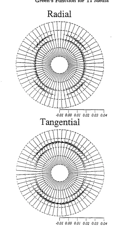
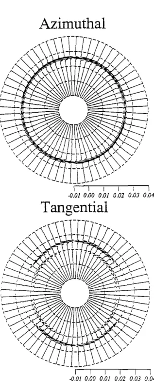
26.6. The parameters of the second medium (plexiglas-aluminum - White, 1984) are: p=1950 kg/rn3

, Cll = 51.8, C33= 21.4, C44 = 3.65, and eBB = 14.1. The first medium is only slightly anisotropic, while the second medium is extremely anisotropic. The displacements are calculated at receivers placed circularly around the sources. For the case of horizontal force, the receiver array makes a 45° azimuthal angle with the x - z plane. The radius of the receiver array is 75 rn for the first medium and 30 rn for the second. The calculated displacements are then rotated to the spherical coordinates. The resulting radial, tangential, and azimuthal components are plotted in a way to show hoth the amplitudes and phase fronts.

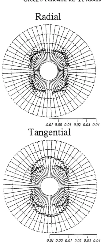
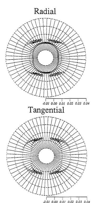
Figure 1, Figures 2 and 3, and Figure 4, respectively, show the displacements due to a vertical, horizontal (x), and explosive point source in the first medium. The phase fronts of the P, SV, and SH waves are almost circular. The P and SH (azimuthal component in Figure 3) waves travel a little faster in the horizontal direction than in the vertical direction. The SV wave travels faster in the 45° direction. That the P and'SV waves sustain large amplitudes in tgeh wide angle range (Figure 1) suggests large lobes in the radiation pattern. Figure 4 shows the existence of SV waves for an explosion in the medium. Ifexamined carefully, this SV wave exhibits two lobes in each quadrant. A similar pattern can also be seen for the vertical force (Figure 1). However, this phenomenon is absent for the case of horizontal force.

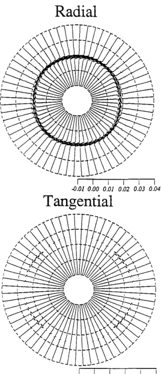
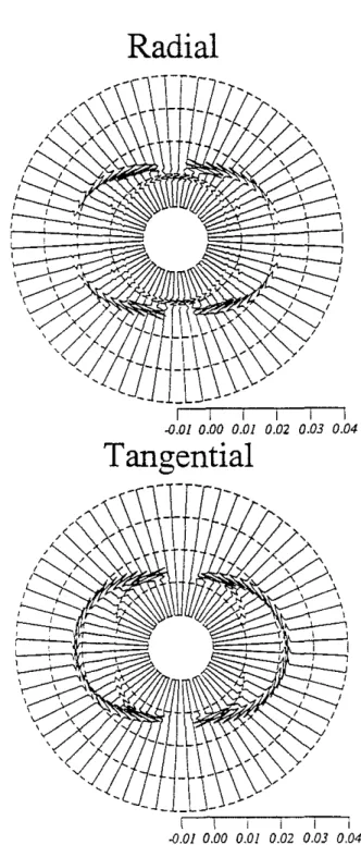
Figures 5-8 show the displacements in the second medium. One immediate ob-servation is the triplication of SV waves. Although the magnitude of one branch is significantly smaller than the other two, three branches of SV wave are clearly seen on Figure 6, where the point force is in the isotropic plane. If the source is a point force along the symmetry axis or explosion, one branch of the triplication disappears. The vertical force result agrees with the calculation of White (1984) for a line source approximated by a borehole along the symmetry axis. White (1984) also demonstrated the difference in energy fall-off for the quasi-P and quasi-SV waves. Amplitude de-cays as -1 power of distance for the P wave, and as -0.8 for the SV waves near the triplication. Our results support this observation.

SURFACE INTEGRATION OF THE GREEN'S FUNCTIONS

In the boundary element method, integration of the Green's function over boundary sur-faces is a necessary calculation. However, the Green's function is singular when receiver and source coincide. The displacement Green's function has first order singularity which is removable when integrated over the surface. On the other hand, the stress Green's function has a second order singularity and the surface integral is not defined. Then, its principal value has to be used. The contribution of this second order singularity to the integral can be evaluated analytically. When the receiver and the source approach each other, the surface integral of the dynamic Green's function can be regularized using the static Green's function (Kupradze, 1963). The singularity integral of the dynamic Green's function is reduced to the integration of the static Green's function over a half elliptical surface around the source point. The limit as the axes of the elliptical surface go to zero is the singular contribution.

Using the static Green's function, we first calculate the displacement and stress field for the vertical point force. We obtain

Ux = u y = Uz

&¢

- ( Cl3

+

C44) axaz (Cl3

+

C44)Sgn(Z - Zl) { X - xl x - x' }

47CC33C44(V; - vD _Rb[Rb

+

vblz - zlll - Ra[Ra

+

valz - ZIJ] (86)

&¢

- ( Cl3

+

C44) ayaz

(Cl3

+

C44)Sgn(Z - Zl) { y - y' y - y' }

47CC33C44(V; - vD Rb[Rb

+

vblz - z/l) - Ra[Ra

+

valz - z/l] (87)

~¢. ~

Notice that the displacements have first order singularity only when x ->

x!.

The stress

along the 2direction on the surface whose normal is

x,

Txz , is

[

aU

z Oux]

Txz

=

C44 ax

+

az

= -1 {Cll+ Cl3 V; X - X ' _ Cll+ Cl3V;X-X/} (89)

47CC33(V; - V~) Va R~ Vb R g '

The stress has second order singularity when the receiver point coincides with the source point (Ra

=

0 and Rb

=

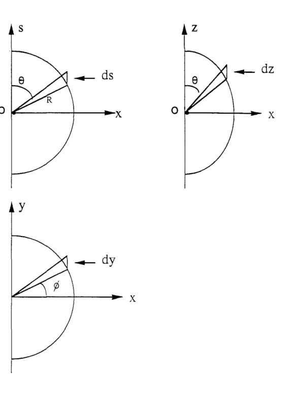
0). Ifthis stress is integrated over a surface that includes the source, a finite value results. This value can be obtained by integrating T_xz over all possible dydz surrounding the source. This integration can be replaced by integration over a half ellipSOidal surface around the source point. The ellipSOidal surface is defined by

X-X' = Rsin Bcos cp, y-y'=RsinBsincp, z-z'=!:.RcosB. (90) V

Using s = ZlZ, the ellipsoidal surface can be transformed into a spherical surface in the (x, y, s) system. Then, surface mapping between dydz and a differential ellipsoidal surface is

dydzsin () cosep

=

"l-dydssin () cosep

=

"l-

R 2sin()d()dep,

ZI ZI (91)

as shown in Figure 9, where, dz = tds, ds = Rd()/sin() and dy = Rsin()dep/cosep. Then,

J

T"zdydz

=

-1 (cn

+

CI3Z1; _ Cn

+

CI3Z1~)

1

tr

/2dep ["sin()d()

411"C33(ZI~ - ZI~) ZI~ ZI~ -tr/2)0

- c n 1

=

2C33Z1~ZI~

=

-2"

(92)

For a point force in the:i: direction, we have

[j2 1

uy - 8x8y

'Vi

(Lt1> - g)

Sb (x - x')(y - y') Sa (x - x')(y - y') ZIg (x - x')(y - y')

Zlb

D~Rb

- Zla

D~Ra

+

411"C66

D~Rg'

8

2¢ Uz = -(CI3

+

C44)8x8z

(

X-X'

X-X')

-Se DbRb - DaRa sgn(z - z'). (94) (95) In the above equations, Da

=

Ra

+

Zlalz -

z'l

and Db

=

Ra

+

Zlblz -

z'l.

The scalars Sa, Sb and Se are

S C44 - C33ZI~ b= 411"C33C44(ZI~ _ ZI~)'

Se = CI3

+

C44

411"C33C44(ZI~ - ZI~)' (96) Then, the normal stress, Txx , is

T_xx = Cn ₍-Bu"

+ -

Buy)

-

2C66-8uy

+

C I 3 -8uz

8x 8y 8y 8z

_ CnSa x - x' 2C66Sa (x - x' _ (x - x')(y - y')2 _ 2(x _ x')(y _ y')2)

Zla R3_a

+

_Zla P D2 D2R3 R2D3

(97)

+

CllSb X - x' _ 2C66Sb (x - x' _ (x - X')(y - y')2 _ 2(x - x')(y _ y')2)

lib R 3 lib RbD2 _{D2 R 3 R}2_D3

b b bb bb

_ IIg (x -

X _

(x - X')(y - y')2 _ 2(x - X')(y _ y')2)

27l" RgD~ D2R~ R~D2

S ₍lIb(X - X) lIa(X - x'»)

+C13 c R3 - R3 .

b a

Similarly, integrating rxx over a small half ellipsoidal surface results in -1/2. This is so because integration of the second, the fourth, the fifth and the last term is zero, as shown in Appendix A, while integration of the first and third term is the same as in rxz for the vertical force.

CONCLUSIONS

The dynamic and static Green's functions have been obtained by solving the wave and equilibrium equations with general sources in a transversely isotropic elastic medium. The use of an extended Kupradze method makes possible a simplified, yet rigorous derivation. The two Green's functions are shown to have a single dyadic form expressed through three scalars: 9for theSHwave,

rP

for theP-SVwaves, and

'l/J

forP-SV -SH waves. In deriving these functions, the 2-D inverse Laplacian operator is removed to ob-tain simplified and numerically feasible expressions for the Green's functions. The final result is valid for arbitrary sources at arbitrary locations. This is particularly important to BEM implementation of wave propagation and scattering problems. The dynamic Green's function is applied to obtain simple analytical expression for the displacements produced by three point sources. Evaluations of these displacements show agreement with previous numerical studies. The singular contribution, when integrating stresses over a half elliptical surface at the limit of the receiver coinciding with the source, is shown to be negative one-half of the applied force.

ACKNOWLEDGEMENTS

Part of the work was accomplished at Mobil Exploration and ProdUcing Technical Cen-ter (MEPTEC) as a second project when the first author was a summer student (1992). He would like to thank Dr. Terry Young of MEPTEC for his encouragement. We thank MEPTEC for te permission for this publication. We are also grateful to Prof. Michel Bouchon (University of Grenoble, France) and Dr. Bata MandaI (M.LT.) for their com-ments.

REFERENCES

Ben-Menahem, A., and A.G. Sena, 1990, Seismic source theory in stratified anisotropic media, J. Geophys. Res., 95, 15,395-15,427.

Ben-Menahem, A., and S.J. Singh, 1981, Seismic Waves and Sources, Springer-Verlag New York Inc., New York.

Bouchon, M., 1992, A numerical simulation of the acoustic and elastic wavefields radi-ated by a source in a fluid-filled borehole embedded in a layered medium, submitted to Geophysics.

Buchwald, V.T., 1959, Elastic waves in anisotropic media, Proc. R. Soc. London, Ser. A, 253, 563-580.

Crampin, S., 1985, Evaluation of anisotropy by shear wave splitting, Geophysics, 50, 383-411.

Dong, W., M. Bouchon, and M.N.. Toks6z, 1992, Modeling downhole source radiation by boundary element and discrete wave number method, SEG Expanded Abstracts, New Orleans, 1337-1340.

Fedorov, F.I., 1968, Theory of Elastic Waves in Crystals, Plenum, New York.

Mandai, B., and M.N. Toks6z, 1990, Computation of complete waveforms in general anisotropic media - Results from an explosion source in anisotropic medium, Geo-phys. J. Int., 103,33--45.

Kazi-Aoual, M.N., G. Bonnet, and P. Jouanna, 1988, Response of an infinite elastic transversely isotropic medium to a point force. An analytical solution in Hankel space, Geophys. J. 93, 587-590.

Kupradze, V.D., 1963, Dynamical Problems in Elasticity, Volume III in Progress in Solid Mechanics, North-Holland, Amsterdam.

Kupradze, V.D., 1979, The Three-Dimensional Problems of the Mathematical Theory of Elasticity and Thermoelasticity, North-Holland, Amsterdam.

Love, A.E.H., 1944, A Treatise on the Mathematical Theory of Elasticity (4th edition). Dover, New York, N.Y., 643 pp.

Pan, Y.C., and T.W., Chou, 1976, Point source solution for an infinite transversely isotropic solid, Transac. Amer. Soc. Mechan. Engineers, December, 608--{)12. Sena, A.G., 1992, Elastic wave propagation in anisotropic media: source theory,

MA 02139.

Watson, G.N., 1944, A 1'reatise on the Theory of Bessel F'unctions, Cambridge Univ. Press, 2nd edition, 1966.

White, J.E., 1983, Underground 8ound: Application of Seismic Waves, Elsevier, Ams-terdam.

White, J .E., 1984, Computed waveforms in transversely isotropic media I: line source and vertical point force, Colo. 8ch. Mines. Quarterly, 79, 33--60.

White, J. E., C. Tongtaow, and C. Monash, 1984, Computed waveforms in transversely isotropic media II: horizontal point force, Colo. 8ch. Mines. Quarterly, 79, 33--60.

APPENDIX A: PROOF OF ZERO INTEGRALS

I =

=

I =

In this appendix, we prove that integrating the second term in equation (97) over a half elliptical surface results in zero. According to Eqs. (90) and (91), we have

J (

dydz X - x'R D2 - (x - x')(y - y')2D2R3 - 2(x - x')(y _ yl)2)R2D3

a u a a a a

1

fa" .

1"/2

(R~

(y - y')2 2Ra(y - y')2)

= -

smBdB dcp - - -

-='=~-Va 0 -"/2 D~ D~ Dg

1 ["

1"/2

( s i n B sin3Bsin

2

cp 2sin3Bsin

2

cp) va)o dB -"/2dcp (1 +

I

cosBf)2 - (1 +

I

cosBf)2 - (1 +

I

cos BIl3

=

!!...- ("

dB ( sinB _ sin3B _ sin3B )

Va)0 (1 +

I

cosBf)2 2(1 +

I

cos BIl2 (1 +

I

cos BIl3 .

Ifwe divide the B integral into two regions, 0 to 71"12 and 71"12 to 71", and combine the first and the third term, we obtain

!!...-

["/2 sinBcosB dB

_!!...- ["

sinBcosB dB

Va )0 (1 + cosB)2 Va ),,/2 (1 - cosB)2 71"

fa"

/2 sin 3

B

71"

1"

sin3

B

- - d B - - dB 2va 0 (1 + cosB)2 2va "/2 (1 - cosB)2

271"

fa"

/2 sinBcosB 71"

fa"

/2 sin3B

- dB-- dB

Va 0 (1 + cosB)2 Va 0 (1 + cosB)2

471"

fa"/4

sin

3

t

271"

fa"/4

(sint

sin

3

t)

- -

- - d t + -

- - - dt

Va 0 cos

t

Va 0 cos

t

cos3

t

471" [ 2 "/4 271" [ ]"/4

- - COS

tl2

-lncost]O + - -In

cost

0

Va Va

271" 1 "/4 --[2 2 +lncost]O

Va COS

t

o.

Radial

I I I I I I .{J.Ol 0.00 0.01 0.02 0.03 0.04

Tangential

--_ T_

I I I I I r .{J.Dl 0.00 0.01 0.02 0.03 0.04

Figure 1: The radial and tangential components of the displacement produced by a point force along the symmetry axis (vertical) in a slightly anisotropic medium: Mesaverde sandstone. The wave amplitudes are normalized to the same scale. Receivers are 75 m away and time is in seconds.

Radial

I I I I I I -0.01 0.00 0.01 0.02 0.03 0.04

Tangential

/ I I I I I I -0.01 0.00 0.01 0.D2 0.03 0.04

Figure 2: The radial and tangential components of the displacement produced by a point force along the isotropic plane (horizontal) in Mesaverde sandstone. Receivers are 75 m away at 45° azimuth angle from the force direction.

Azimuthal

/ I I I I I I -0.01 0.00 0.01 0.02 0.03 0.04

Tangential

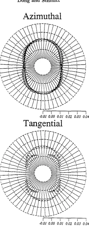
I I I 0.02 0.03 0.04

Figure 3: The azimuthal (SH wave) and tangential components of the displacement produced by a point force along the isotropic plane (horizontal) in Mesaverde sand-stone. Same receiver position as Figure 2.

Radial

I I I I I I -<J.Ol 0.00 0.01 0.02 0.03 0.04

Tangential

,

I I I I I I -<J.Ol 0.00 0.01 0.02 0.03 0.04

Figure 4: The radial and tangential components of the displacement produced by an explosion in Mesaverde sandstone.

Radial

I I I I I I -0.01 0.00 0.01 0.02 0.03 0.04

Tangential

f

-I I I I I I -0.01 0.00 0.01 0.02 0.03 0.04 (

Figure 5: The radial and tangential components of the displacement produced by a point force along the symmetry axis (vertical) in a highly anisotropic medium: plexiglas-aluminum. Receivers are 30 m away from the source.

Radial

I I I I I I -0.01 0.00 0.01 0.02 0.03 0.04

Tangential

I I I i -O.oI 0.00 0.0/ 0.02 0.D3 0.04

Figure 6: The radial and tangential components of the displacement produced by a point force along the isotropic plane (horizontal) in plexiglas-aluminum. Receivers are 30 m away at 45° azimuth angle from the force direction.

Azimuthal

I I I I I I

-0,0] 0.00 0.01 0.02 0.03 0.04

I I I I I I

-0.01 0.00 0.01 0.02 0.03 0.04

Figure 7: The azimuthal (SH wave) and tangential components of the displacement pro-duced by a point force along the isotropic plane (horizontal) in plexiglas-aluminum. Same receiver position as Figure 6.

Radial

I I I I I I

-0.01 0.00 0.01 0.02 0.03 0.04

I I I I I I

-0.01 0.00 0.01 0.02 0.03 0.04

Figure 8: The radial and tangential components of the displacement produced by an explosion in plexiglas-aluminum.

o

s

__ ds

~----+---x

y

o

z

__ dz

x

__ dy

x

Figure 9: The geometry of the differential surfaces used in evaluating the singular contrihution of surface integration of Green's functions.