HAL Id: hal-00318184
https://hal.archives-ouvertes.fr/hal-00318184
Submitted on 20 Oct 2006
HAL is a multi-disciplinary open access
archive for the deposit and dissemination of
sci-entific research documents, whether they are
pub-lished or not. The documents may come from
teaching and research institutions in France or
abroad, or from public or private research centers.
L’archive ouverte pluridisciplinaire HAL, est
destinée au dépôt et à la diffusion de documents
scientifiques de niveau recherche, publiés ou non,
émanant des établissements d’enseignement et de
recherche français ou étrangers, des laboratoires
publics ou privés.
The role of the zonal ExB plasma drift in the
low-latitude ionosphere at high solar activity near
equinox from a new three-dimensional theoretical model
A. V. Pavlov
To cite this version:
A. V. Pavlov. The role of the zonal ExB plasma drift in the low-latitude ionosphere at high solar
activity near equinox from a new three-dimensional theoretical model. Annales Geophysicae, European
Geosciences Union, 2006, 24 (10), pp.2553-2572. �hal-00318184�
Ann. Geophys., 24, 2553–2572, 2006 www.ann-geophys.net/24/2553/2006/ © European Geosciences Union 2006
Annales
Geophysicae
The role of the zonal E×B plasma drift in the low-latitude
ionosphere at high solar activity near equinox from a new
three-dimensional theoretical model
A. V. Pavlov
Pushkov Institute of Terrestrial Magnetism, Ionosphere and Radio-Wave Propagation, Russian Academy of Science (IZMIRAN), Troitsk, Moscow Region, 142190, Russia
Received: 2 May 2006 – Revised: 22 August 2006 – Accepted: 31 August 2006 – Published: 20 October 2006
Abstract. A new three-dimensional, time-dependent theo-retical model of the Earth’s low and middle latitude iono-sphere and plasmaiono-sphere has been developed, to take into account the effects of the zonal E×B plasma drift on the elec-tron and ion number densities and temperatures, where E and B are the electric and geomagnetic fields, respectively. The model calculates the number densities of O+(4S), H+, NO+, O+2, N+2, O+(2D), O+(2P), O+(4P), and O+(2P*) ions, the electron density, the electron and ion temperatures using a combination of the Eulerian and Lagrangian approaches and an eccentric tilted dipole approximation for the geomagnetic field. The F2-layer peak density, NmF2, and peak altitude,
hmF2, which were observed by 16 ionospheric sounders
dur-ing the 12–13 April 1958 geomagnetically quiet time high solar activity period are compared with those from the model simulation. The reasonable agreement between the measured and modeled NmF2 and hmF2 requires the modified equato-rial meridional E×B plasma drift given by the Scherliess and Fejer (1999) model and the modified NRLMSISE-00 atomic oxygen density. In agreement with the generally accepted as-sumption, the changes in NmF2 due to the zonal E×B plasma drift are found to be inessential by day, and the influence of the zonal E×B plasma drift on NmF2 and hmF2 is found to be negligible above about 25◦ and below about –26◦ geo-magnetic latitude, by day and by night. Contrary to common belief, it is shown, for the first time, that the model, which does not take into account the zonal E×B plasma drift, un-derestimates night-time NmF2 up to the maximum factor of 2.3 at low geomagnetic latitudes, and this plasma transport in geomagnetic longitude is found to be important in the cal-culations of NmF2 and hmF2 by night from about –20◦ to
about 20◦geomagnetic latitude. The longitude dependence of the night-time low-latitude influence of the zonal E×B plasma drift on NmF2, which is found for the first time, is
Correspondence to: A. V. Pavlov
(pavlov@izmiran.rssi.ru)
explained in terms of the longitudinal asymmetry in B (the eccentric magnetic dipole is displaced from the Earth’s cen-ter and the Earth’s eccentric tilted magnetic dipole moment is inclined with respect to the Earth’s rotational axis) and the variations of the wind induced plasma drift and the merid-ional E×B plasma drift in geomagnetic longitude. The study of the influence of the zonal E×B plasma drift on the topside low-latitude electron density is presented for the first time. Keywords. Ionosphere (Electric fields and currents; Equa-torial ionosphere; Modeling and forecasting; Plasma temper-ature and density)
1 Introduction
The ionosphere at the geomagnetic equator and low geomag-netic latitudes have been studied observationally and theo-retically for many years (see Moffett, 1979; Anderson, 1981; Walker, 1981; Anderson et al., 1996; Bailey and Balan, 1996; Millward et al., 1996; Roble, 1996; Richards and Torr, 1996; Schunk and Sojka, 1996; Rishbeth, 2000; Abdu, 1997, 2001; Huba et al., 2000; Fesen et al., 2002; Maruyama et al., 2003; Pavlov et al., 2006, and references therein). The behaviour of the equatorial and low-latitude ionosphere is strongly de-pendent upon the meridional component (which is located in a plane of a geomagnetic meridian) of a drift velocity, VE=E×B/B2, of electrons and ions perpendicular to the
ge-omagnetic field, B, due to an electric field, E, which is gen-erated in the E region. Sterling et al. (1969) found that the effect of the zonal component of VE(geomagnetic east – ge-omagnetic west component) on the F2-layer peak density in the low-latitude ionosphere is not significant at solar mini-mum and solar maximini-mum equinoctial conditions. However, as was pointed out by Anderson (1981), the zonal plasma drift used by Sterling et al. (1969) bears little resemblance to the observed zonal plasma drifts given by Fejer et al. (1981).
2554 A. V. Pavlov: The role of the zonal E×B plasma drift in the low-latitude ionosphere
This discrepancy between the measured and plasma drifts used can lead to an incorrect conclusion about the role of the zonal component of the E×B plasma drift in the low-latitude ionosphere. The average E×B zonal F-region plasma drift (Fejer et al., 1981) measured over Jicamarca was used by An-derson (1981) to reinvestigate the effects of the zonal E×B plasma drift on the equatorial F-region ionosphere for high solar activity conditions. Anderson (1981) has found that the F2-layer peak electron densities calculated over the geo-magnetic equator at 20:00 LT and at 24:00 LT do not differ significantly from those obtained when the zonal E×B drift is omitted, while there are noticeable changes in the F2-layer peak altitudes (see Fig. 10 of Anderson, 1981). As a result of the model calculations given by Anderson (1981), effects of the zonal E×B plasma drift on the electron and ion densities and temperatures were not taken into account in the previ-ous model studies (e.g. Anderson et al., 1996; Bailey and Balan, 1996; Millward et al., 1996; Pavlov, 2003; Pavlov et al., 2004a, b, 2006). The present work revises the relation-ship between the zonal component of the plasma drift and the dynamics of the low-latitude F2-layer using a new three-dimensional time-dependent model of the low and middle latitude ionosphere and plasmasphere presented in Sect. 2. To test the reliability of the new model, the theoretical study is carried out in the present case study, in which the F2-layer peak electron density, NmF2, and altitude, hmF2, are observed simultaneously in the low-latitude ionosphere by the La Paz, Trivandrum, Ahmedabad, Kodaikonal, Tiruchi-rapalli, Singapore, Maui, Panama, Talara, Chiclayo, Huan-cayo, and Bogota ionospheric sounders during the 12–13 April 1958 geomagnetically quiet time period at high solar activity.
2 New three-dimensional, time-dependent theoretical model
The two-dimensional, time-dependent model of the low and middle latitude ionosphere and plasmasphere developed by Pavlov (2003) calculates the number densities, Ni, of
O+(4S), H+, NO+, O+2, N2+, O+(2D), O+(2P), O+(4P), and O+(2P*) ions, Ne, the electron, Te, and ion, Ti, temperatures
in a plane of a geomagnetic meridian in a centered dipole approximation for the geomagnetic field without taking into consideration the zonal plasma drift effects on Ni, Ne, Te,
and Ti. A new three-dimensional time-dependent
mathe-matical model of the low and middle latitude ionosphere and plasmasphere presented in this work includes the two-dimensional time-dependent model given by Pavlov (2003) as a principal block, takes into account the effects of the zonal plasma drift on Ni, Ne, Te, and Ti, and uses an
eccen-tric tilted dipole approximation for the geomagnetic field to calculate the time-dependent electron and ion densities, and temperatures as a function of latitude, longitude, and altitude on a fixed spatial grid at low and middle latitudes. In the
model, the Earth’s eccentric tilted magnetic dipole moment is inclined with respect to the Earth’s rotational axis but is lo-cated at a point which is not coincident with the Earth’s cen-ter (the first eight nonzero coefficients in the expansion of the geomagnetic field potential in terms of spherical harmonics are taken into account). The dependences of the parameters of the eccentric tilted magnetic dipole on a year are given by Frazer-Smith (1987) and Deminov and Fishchuk (2000). The model includes the production and loss rates of ions by the photochemical reactions described in detail by Pavlov (2003) and Pavlov and Pavlova (2005).
Eccentric dipole orthogonal curvilinear coordinates q, U, and 3 are employed in the model calculations, where q is aligned with, and U and 3 are perpendicular to, the mag-netic field, and the U and 3 coordinates are constant along an eccentric dipole magnetic field line. It should be noted that q=(RE/R)2cos 2, U=(RE/R) sin22, and 3 is the
geomag-netic longitude, where R is the radial distance from the ge-omagnetic field center, 2=90◦−ϕis the geomagnetic
colati-tude, ϕ is the geomagnetic laticolati-tude, RE is the Earth’s radius.
In the model, VE=VE3 e3+VUE eU, where VE3=EU/B is the
zonal component of VE, VEU=−E3/B is the meridional
com-ponent of VE, E=E
3e3+EU eU, E3is the 3 (zonal)
compo-nent of E in the dipole coordinate system, EUis the U
(merid-ional) component of E in the dipole coordinate system, e3
and eU are unit vectors in 3 and U directions, respectively,
eUis directed downward at the geomagnetic equator.
Equations which determine the trajectory of the iono-spheric plasma perpendicular to magnetic field lines and the moving coordinate system are derived by Pavlov (2003) as
∂ ∂tU = −E eff 3R −1 E B −1 0 , (1) ∂ ∂t3 = E eff UR −1 E B −1 0 , (2)
where Eeff3=E3h3R−E1, EeffU=EU hU R−E1, h3=Rsin 2,
hU=RU−1cos I, RE is the Earth’s radius, I is the magnetic
field dip angle, cos I=sin 2 (1+3cos22)−1/2, B0is the value
of B for R=RE and 2=0.
As a result of the condition of the frozen-in magnetic field lines into the ionospheric and plasmaspheric plasma, the val-ues of the effective zonal and meridional electric fields Eeff3 and EeffU are not changed along magnetic field lines (Pavlov, 2003): ∂ ∂qE eff 3 =0, ∂ ∂qE eff U =0. (3)
It is worth noting that the effective zonal and meridional plasma drift velocities Veff3=EeffU B−01and VeffU=−Eeff3 B−01can be used in Eqs. (1–3) instead of EeffU and Eeff3, respectively, where Veff3=VE3REh−31and VeffU=VEU REh−U1.
The model calculates the values of Ni, Ne, Ti, and Te in
the fixed nodes of the fixed Eulerian volume grid at the fixed
A. V. Pavlov: The role of the zonal E×B plasma drift in the low-latitude ionosphere 2555
universal times UT≡t=t0, t0+1t, t0+21t, and so on, up to the final universal time with the time step 1t. This Eulerian com-putational grid consists of a distribution of the dipole mag-netic field lines in the ionosphere and plasmasphere. One hundred dipole magnetic field lines are used in the model for each fixed value of 3. The number of the fixed nodes taken along each magnetic field line is 191. Seventy-two model Eulerian (q,U) computational grid planes are located at 3=0◦, 5◦,. . . 355◦. For each fixed value of 3, the region of study is a (q,U) plane, which is bounded by two dipole magnetic field lines. The computational grid dipole magnetic field lines are distributed between the low and upper bound-ary lines. Computational grid dipole magnetic field lines intersect the geomagnetic equatorial point (q=0) at the ge-omagnetic equatorial crossing heights h1eq, h2eq, . . . hmmeq with the interval 1hmeq=hmeq−hm−eq 1 between neighboring compu-tational grid lines m and m-1, where m=2,. . . mm, mm=100. The low boundary magnetic field line intersects the geomag-netic equatorial point at the geomaggeomag-netic equatorial crossing height h1eq=150 km. The upper boundary magnetic field line has hmmeq =4264 km.. The computational grid lines have the interval 1hmeq of 20 km for m=1 and m=2, and the value of 1hmeq is increased from 20 km to 42 km linearly, if the value of m is changed from m=3 to m=mm.
At each time point, we use the implementation of the Eulerian-Lagrangian method developed by Pavlov (2003) in solving the time dependent and two-dimensional continu-ity and energy equations at a (q,U) plane and upgrade this method, taking into consideration the plasma drift between the (q,U) planes in geomagnetic longitude. The Eulerian-Lagrangian scheme used describes the plasma evolution based on a reference frame (see Eqs. 1–2) moving with an individual parcel of plasma like a fully Lagrangian method, but makes use an Eulerian computational grid. It involves a forward time integration of Eqs. (1–2). Figure 1 shows schematic illustration of the major elements of the differ-ence between the two-dimensional approach and the three-dimensional approach in the calculations of Ni, Te, and Te
described below.
Let us assume that the values of Ni(q,U,3,t), Ti(q,U,3,t),
and Te(q,U,3,t) are known, and we calculate the values of
Ni(q,U,3,t+1t), Ti(q,U,3,t+1t), and Te(q,U,3, t+1t)
si-multaneously for all the computational grid dipole magnetic field lines. The model calculations are carried out in the two parts at each time step. In the first part, the new model uses the algorithms developed by Pavlov (2003) to describe plasma evolution in each (q,U) plane. However, as dis-tinct from the two-dimensional approach of Pavlov (2003), the three-dimensional model results at t+1t correspond to a (q,U) plane which is located at 3+13, and this change in geomagnetic longitude (the value of 13) is caused by the zonal E×B plasma drift. As a result of the first part, the model calculates the values of Ni(q,U,3k+13k,t+1t),
Ti(q,U,3k+13k,t+1t), and Te(q,U,3k+13k,t+1t) from
the values of Ni(q,U,3k,t), Ti(q,U,3k,t), and Te(q,U,3k,t),
where k=1,2,. . . kk. The magnitude of 13k is determined
from Eq. (2). In the second part, we calculate the values of Ni(q,U,3k,t+1t), Ti(q,U,3k,t+1t), and Te(q,U,3k,t+1t).
In the low-latitude ionosphere, the value of VE3is positive (an eastward drift of plasma) during the most of the daytime con-ditions, while during the most of the night-time concon-ditions, the plasma moves westward perpendicular to the geomag-netic field lines in longitude (Fejer et al., 2005; Fejer, 1993). The subsequent strategy of the second part for the case when VE3>0 is different from that for the case when VE3<0.
At first, we describe the technique in the case when the zonal plasma drift is directed eastward (VE3(q,U,3k,t)>0).
Using the values of Ni(q,U,3k+13k,t+1t),
Ti(q,U,3k+13k,t+1t), Te(q,U,3k+13k,t+1t) and
Ni(q,U,3k−1+13k−1,t+1t), Ti(q,U,3k−1+13k−1,t+1t),
Te(q,U,3k−1+13k−1,t+1t), and the interpolation
pro-cedure, the model calculates the desired quantities of Ni(q,U,3k,t+1t), Ti(q,U,3k,t+1t), and Te(q,U,3k,t+1t).
It should be noted that the quantities of Ni(q,U,31,t+1t),
Ti(q,U,31,t+1t), and Te(q,U,31,t+1t) are found from the
values of Ni(q,U,31+131,t+1t), Ti(q,U,31+131,t+1t),
Te(q,U,31+131,t+1t) and Ni(q,U,3kk+13kk,t+1t),
Ti(q,U,3kk+13kk,t+1t), Te(q,U,3kk+13kk,t+1t), and
the interpolation procedure.
If the plasma moves westward, i.e. VE3(q,U,3k,t)<0,
then the technique is changed in comparison with the previous case. The values of Ni(q,U,3k+13k,t+1t),
Ti(q,U,3k+13k,t+1t), Te(q,U,3k+13k,t+1t) and
Ni(q,U,3k−1+13k+1,t+1t), Ti(q,U,3k+1+13k+1,t+1t),
Te(q,U,3k+1+13k+1,t+1t), and the interpolation
pro-cedure are used to calculate the desired quantities of Ni(q,U,3k,t+1t), Ti(q,U,3k,t+1t), and Te(q,U,3k,t+1t).
Using the interpolation procedure, the values of Ni(q,U,3kk,t+1t), Ti(q,U,3kk,t+1t), and Te(q,U,3kk,t+1t)
are determined from the values of Ni(q,U,3kk+13kk,t+1t),
Ti(q,U,3kk+13kk,t+1t), Te(q,U,3kk+13kk,t+1t)
and Ni(q,U,31+131,t+1t), Ti(q,U,31+131,t+1t),
Te(q,U,31+131,t+1t).
If VE3(q,U,3k,t)=0, then the desired values of
Ni(q,U,3k,t+1t), Ti(q,U,3k,t+1t), and Te(q,U,3k,t+1t)
are calculated from Ni(q,U,3k,t), Ti(q,U,3k,t), and
Te(q,U,3k,t), without taking into account the plasma drift
between the (q,U) planes in geomagnetic longitude.
As a result, the two-dimensional Eulerian-Lagrangian scheme of Pavlov (2003) was extended to the three-dimensional scheme. The new model works as a time de-pendent three-dimensional (q, U, and 3 coordinates) global model of the low and middle latitude ionosphere and plasma-sphere.
Equations (1–2) determine the trajectory of the iono-spheric plasma perpendicular to the magnetic field lines and the moving coordinate system. Time variations of U are de-termined by time variations of Eeff3, and time variations of 3
2556 A. V. Pavlov: The role of the zonal E×B plasma drift in the low-latitude ionosphere VEΛ(q,U,Λk,t)>0 k=2,…kk Ni(q,U,Λk,t), Ti(q,U,Λk,t), Te(q,U,Λk,t) Ni(q,U,Λk+∆Λk,t+∆t), Ti(q,U,Λk+∆Λk,t+∆t), Te(q,U,Λk+∆Λk,t+∆t) Ni(q,U,Λk-1+∆Λk-1,t+∆t), Ti(q,U,Λk-1+∆Λk-1,t+∆t), Te(q,U,Λk-1+∆Λk-1,t+∆t) Ni(q,U,Λk-1,t), Ti(q,U,Λk-1,t), Te(q,U,Λk-1,t) Ni(q,U,Λk,t+∆t), Ti(q,U,Λk,t+∆t), Te(q,U,Λk,t+∆t) k=1 Ni(q,U,Λ1+∆Λ1,t+∆t), Ti(q,U,Λ1+∆Λ1,t+∆t), Te(q,U,Λ1+∆Λ1,t+∆t) Ni(q,U,Λkk,t), Ti(q,U,Λkk,t), Te(q,U,Λkk,t) Ni(q,U,Λ1,t+∆t), Ti(q,U,Λ1,t+∆t), Te(q,U,Λ1,t+∆t) Ni(q,U,Λ1,t), Ti(q,U,Λ1,t), Te(q,U,Λ1,t) Ni(q,U,Λkk+∆Λkk,t+∆t), Ti(q,U,Λkk+∆Λkk,t+∆t), Te(q,U,Λkk+∆Λkk,t+∆t) VEΛ(q,U,Λk,t)<0 k=1,…kk-1 k=kk Ni(q,U,Λk,t), Ti(q,U,Λk,t), Te(q,U,Λk,t) Ni(q,U,Λk+∆Λk,t+∆t), Ti(q,U,Λk+∆Λk,t+∆t), Te(q,U,Λk+∆Λk,t+∆t) Ni(q,U,Λk,t+∆t), Ti(q,U,Λk,t+∆t), Te(q,U,Λk,t+∆t) Ni(q,U,Λkk+∆Λkk,t+∆t), Ti(q,U,Λkk+∆Λkk,t+∆t), Te(q,U,Λkk+∆Λkk,t+∆t) Ni(q,U,Λ1+∆Λ1,t+∆t), Ti(q,U,Λ1+∆Λ1,t+∆t), Te(q,U,Λ1+∆Λ1,t+∆t) Ni(q,U,Λk+1,t), Ti(q,U,Λk+1,t), Te(q,U,Λk+1,t) Ni(q,U,Λk+1+∆Λk+1,t+∆t), Ti(q,U,Λk+1+∆Λk+1,t+∆t), Te(q,U,Λk+1+∆Λk+1,t+∆t) Ni(q,U,Λkk,t), Ti(q,U,Λkk,t), Te(q,U,Λkk,t) Ni(q,U,Λ1,t), Ti(q,U,Λ1,t), Te(q,U,Λ1,t) Ni(q,U,Λkk,t+∆t), Ti(q,U,Λkk,t+∆t), Te(q,U,Λkk,t+∆t) Fig. 1 25
Fig. 1. The major elements of the difference between the two-dimensional approach (Pavlov, 2004) and the three-dimensional approach used
in this work in calculations of Ni, Te, and Ti.
are determined by time variations of EeffU. In the model cal-culations, the empirical F-region quiet time equatorial ver-tical drift model of Scherliess and Fejer (1999) is used to calculate the value of E3 over the geomagnetic equator at
F-region altitudes. The time variations of EU used in the
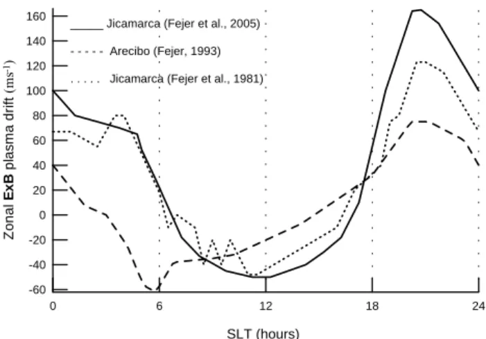
model simulations over the geomagnetic equator at F-region altitudes are obtained from the time variations of the empir-ical F-region quiet time equatorial zonal plasma drift shown by the solid line in Fig. 2. The value of this drift velocity is taken from Fig. 2 of Fejer et al. (2005) over Jicamarca for
A. V. Pavlov: The role of the zonal E×B plasma drift in the low-latitude ionosphere 2557
equinox conditions and F10.7=180. It is assumed that this value of EU is the same at all geomagnetic longitudes over
the geomagnetic equator at F-region altitudes. The equato-rial electric fields E3and EU are used to find the equatorial
effective electric fields Eeff3 and EeffU.
The dashed line in Fig. 2 shows the average quiet time zonal plasma drift velocity over Arecibo for equinox con-ditions at solar maximum taken from Fig. 3 of Fejer (1993). This drift is used to determine the value of EUat the F-region
altitudes over Arecibo. The average quiet time electric field E3at the F-region altitudes over Arecibo is found from the
average quiet time perpendicular/northward F-region plasma drift for equinox conditions at solar maximum presented in Fig. 2 of Fejer (1993). The Arecibo values of E3 and EU
are used to find the Arecibo quantities of Eeff3 and EeffU. Let a geomagnetic field line intersect the 300-km altitude over the Arecibo radar at a geomagnetic latitude of ϕA. The values
of Eeff3 and EeffU are assumed to be the same in the considered (q,U) planes for magnetic field lines which intersect the 300-km altitude at geomagnetic latitudes ϕ≥ϕA. The equatorial
effective electric fields Eeff3 and EeffU are used for magnetic field lines, which intersect the geomagnetic equatorial points at the geomagnetic equatorial crossing heights hkeq≤500 km. Linear interpolation of the equatorial and Arecibo quantities of Eeff3 and EeffU are employed at intermediate dipole magnetic field lines.
The finite-difference algorithm described above yields ap-proximations to Ni, Ne, Ti, and Te in the ionosphere and
plasmasphere at 72 Eulerian computational grid (q,U) planes with the time step 1t=10 min. The interpolation procedure is used to find the values of Ni, Ne, Ti, and Te at points
which are located between 72 Eulerian computational grid (q,U) planes. Using initial ion densities, and electron and ion temperatures, the model is run from 14:00 UT on 10 April 1958 to 24:00 UT on 13 April 1958. To neglect the effects of the initial conditions on Ni, Ti, and Te, the values of Ni, Ti,
and Te produced by the model from 14:00 UT on 10 April
1958 to 24:00 UT on 11 April 1958 are not taken into con-sideration, and the model results are used during the studied time period from 00:00 UT on 12 April 1958 to 24:00 UT on 13 April 1958. As the model inputs, the horizontal com-ponents of the neutral wind are specified using the HWM90 wind model (Hedin et al., 1991), the model solar EUV fluxes are taken from the EUVAC model (Richards et al., 1994), while neutral densities and temperature are taken from the NRLMSISE-00 model (Picone et al., 2002).
3 Solar geophysical conditions and data
The characteristic time of the neutral composition recovery after a storm impulse event ranges from 7 to 12 h, on average (Hedin, 1987), while it may need up to several days for all altitudes down to 120 km in the atmosphere to recover com-pletely back to the undisturbed state of the atmosphere
(Rich-0 6 12 18 24 SLT (hours) Fig. 2 -60 -40 -20 0 20 40 60 80 100 120 140 160 Zo n a l Ex B pl as m a d rif t (m s -1)
_____ Jicamarca (Fejer et al., 2005) - - - Arecibo (Fejer, 1993) . . . Jicamarca (Fejer et al., 1981)
26
Fig. 2. Diurnal variations of the quiet time zonal E×B plasma drift
velocity at F-region altitudes over Jicamarca (solid and dotted lines) and over Arecibo (dashed line) for equinox conditions at solar max-imum. The Jicamarca zonal E×B plasma drift velocity are taken from Fig. 2 of Fejer et al. (2005) (solid line) and from Fig. 2 of Fejer et al. (1981) (dotted line), while the dashed line represents the Arecibo data presented in Fig. 3 of Fejer (1993). The zonal
E×B plasma drifts shown by the solid and dashed lines are used
in the model simulations of this work (see Sect. 2), while the data presented by the dotted line were used by Anderson (1981) (see discussion in Sect. 4). SLT is the solar local time (SLT=UT+ψ/15, where ψ is the geographic latitude).
mond and Lu, 2000). The value of the geomagnetic Kp index was in the range from 1−to 30during 10–11 April 1958 and
between 0+ and 3− during 12–13 April 1958. Therefore,
the studied time period of 12–13 April 1958 can be consid-ered as a geomagnetically quiet time period. The F10.7 solar activity index was equal to 197 on 12 April and 181 on 13 April, while the 81-day averaged F10.7 solar activity index centered on 12 or 13 April was close to 244.
Hourly critical frequencies, foF2 and foE, of the F2 and E layers, and maximum usable frequency parameter, M(3000)F2, from the La Paz, Natal, Bombay, Ahmedabad, Trivandrum, Kodaikonal, Tiruchirapalli, Delhi, Calcutta, Singapore, Maui, Talara, Panama, Chiclayo, Huancayo, and Bogota ionospheric sounder stations, which are available at the Ionospheric Digital Database of the National Geophys-ical Data Center, Boulder, Colorado, are used as a base for the purpose of this investigation. The locations of these iono-spheric sounder stations are shown in Table 1. The value of the peak density, NmF2, of the F2 layer is related to the crit-ical frequency foF2 as NmF2=1.24×10¹⁰ foF22, where the unit of NmF2 is m−3, the unit of foF2 is MHz. To determine the ionosonde value of hmF2, the relation between hmF2 and the values of M(3000)F2, foF2, and foE recommended by Dudeney (1983) is used as hmF2=1490/[M(3000)F2+1M]– 176, where 1M=0.253/(foF2/foE-1.215)–0.012. If there are no foE data, then it is suggested that 1M=0, i.e. the hmF2 formula of Shimazaki (1955) is used. The reliability of hmF2
2558 A. V. Pavlov: The role of the zonal E×B plasma drift in the low-latitude ionosphere
Table 1. Ionosonde station names and locations, and the maximum model value of NmF2/NmF2(VE3=0) over each ionosonde station during 12–13 April 1958. Geomagnetic latitudes and longitudes are calculated in eccentric (first number) and centered (second number) dipole approximations for the geomagnetic field using the parameters of these magnetic field approximations for the time period 1958.
Ionosonde Geographic Geographic Geomagnetic Geomagnetic [NmF2/NmF2(EU=0)]max
Stations latitude longitude latitude longitude
La Paz −16.5 291.9 −5.2, −5.0 3.4, 1.2 1.2 Natal −5.3 324.9 3.5, 4.2 34.4, 34.2 1.2 Bombay 19.0 72.8 9.5, 9.8 140.1, 143.8 2.4 Ahmedabad 23.0 72.6 13.6, 13.8 140.3, 145.8 2.1 Trivandrum 8.5 77.0 −1.6, −1.1 143.0, 146.8 2.3 Kodaikonal 10.2 77.5 0.1, 0.5 143.7, 147.4 2.3 Tiruchirapalli 10.8 78.7 0.6, 1.0 144.9, 148.7 2.3 Delhi 28.6 77.2 18.8, 18.8 145.3, 149.2 1.5 Calcutta 23.0 88.6 12.2, 12.3 155.7, 159.3 2.2 Singapore 1.3 103.8 −11.1, −10.1 170.1, 173.0 2.1 Maui 20.8 203.5 21.4, 20.9 271.8, 268.4 1.1 Talara −4.5 278.6 6.0, 6.8 350.8, 347.9 1.5 Panama 9.4 280.1 19.4, 20.7 351.9, 348.9 1.1 Chiclayo −6.7 280.1 4.0, 4.6 352.3, 349.5 1.5 Huancayo −12.0 284.6 −1.0, −0.6 356.7, 354.1 1.4 Bogota 4.5 285.8 14.8, 16.0 357.6, 355.0 1.2
derived from the observed values of M(3000)F2, foF2, and
foE by means of the Dudeney (1983) approach is supported
by the reasonable agreement between these values of hmF2 and those measured by the middle and upper atmosphere radar at Shigaraki (34.85◦N, 136.10◦E) during 19–21 March 1988 and 25–27 August 1987 (Pavlov et al., 2004a, b).
4 Model/data comparisons
The measured (squares) and calculated (lines) NmF2 and
hmF2 are displayed in Figs. 3–6 from 00:00 UT on 12 April
to 24:00 UT on 13 April above the ionosonde stations pre-sented in Table 1. For clarity, the solar local time, SLT, is used in Figs. 3–6 for each ionosonde station (SLT=UT+ψ /15, where ψ is the geographic latitude). The NRLMSISE-00 neutral temperature and densities, and the equatorial E3
given by the equatorial perpendicular plasma drift model of Scherliess and Fejer (1999) for the studied time period are used in producing the model results shown by dashed lines in Figs. 3–6. Solid and dotted lines show the results from the model with the corrected E3and NRLMSISE-00 atomic
oxygen density, which are discussed below. The zonal com-ponent of the plasma drift described in Sect. 2 is taken into account in the model results shown by solid and dashed lines in Figs. 3–6, while dotted lines in Figs. 3–6 are produced by the model when the zonal plasma drift is equal to zero.
Close to the geomagnetic equator, the meridional wind has little effect on the spatial and temporal features of the dis-tribution of plasma, and the meridional E×B plasma drift
is the primary force in determining hmF2 (Rishbeth, 2000; Souza et al., 2000; Pavlov, 2003; Pavlov et al., 2004a, b). As a result, it is necessary to compare the measured and mod-eled hmF2 close to the geomagnetic equator to adjust the value of E3for the studied time period. The comparison
be-tween the measured hmF2 shown by the squares in Figs. 3– 6 and the calculated hmF2 shown by the dashed lines in Figs. 3–6 clearly indicates that there is a large disagreement between the measured and modeled hmF2 over the Natal, Ahmedabad, Talara, and Chiclayo ionosonde stations close to 18:00–20:00 SLT on 12 and 13 April 1958 if the equato-rial E3determined by the plasma drift model of Scherliess
and Fejer (1999) is used. It follows from the model sim-ulations that it is unlikely to make the measured and mod-eled hmF2 over these ionosonde stations agree via changes in the neutral wind, densities, and temperature. The model of the ionosphere and plasmasphere overestimates hmF2 un-der conditions of strong upward plasma drifts before and dur-ing the evendur-ing prereversal plasma drift enhancement, trans-porting ions and electrons from lower to higher altitudes. Therefore, if the equatorial perpendicular plasma drift given by the empirical model of Scherliess and Fejer (1999) at each geomagnetic longitude over the geomagnetic equator exceeds 20 ms−1from 16:00 SLT to 20:00 SLT, then it is set to 20 ms−1, to improve the agreement between the measured and modeled hmF2 over the Natal, Ahmedabad, Talara, and Chiclayo ionosonde stations.
Figures 3–6 show that the modeled daytime values of
NmF2, given by dashed lines, are overestimated in
compar-ison with the observed values. It can be expected that the
A. V. Pavlov: The role of the zonal E×B plasma drift in the low-latitude ionosphere 2559 300 400 500 600 700 hm F2 (km) 22 4 10 16 22 4 10 16 SLT (hours) 10 20 30 40 50 Nm F2 (10 5 cm -3) 300 400 500 600 hm F2 ( k m ) 20 2 8 14 20 2 8 14 SLT (hours) 10 20 30 40 Nm F2 ( 1 0 5 cm -3) -5.2° and 3.4° geomagnetic
latitude and longitude
3.5° and 34.4° geomagnetic
latitude and longitude La Paz Natal 5 11 17 23 5 11 17 23 SLT (hours) 5 11 17 23 5 11 17 23 SLT (hours) Fig. 3
9.5° and 140.1° geomagnetic latitude
and longitude
Bombay
13.6° and 140.3° geomagnetic
latitude and longitude Ahmedabad Ahmedabad La Paz Natal Bombay 27
Fig. 3. Observed (squares) and calculated (lines) NmF2 and hmF2 above the La Paz, Natal, Bombay, and Ahmedabade ionosonde stations
from 00:00 UT on 12 April 1958 to 24:00 UT on 13 April 1958. SLT is the solar local time at each ionosonde station. The results obtained from the model of the ionosphere and plasmasphere using the equatorial E3, produced by the equatorial perpendicular plasma drift model of Scherliess and Fejer (1999), and the NRLMSISE-00 neutral temperature and densities, as the input model parameters, are shown by dashed lines. Solid and dotted lines show the results given by the model with the corrected equatorial E3and the NRLMSISE-00 model with the corrected value of [O]. The corrected meridional E×B plasma drift given by the model of Scherliess and Fejer (1999) is taken to be 20 ms−1from 16:00 SLT to 20:00 SLT at each geomagnetic longitude over the geomagnetic equator, if this drift is larger than 20 ms−1. The NRLMSISE-00 model atomic oxygen number density was decreased by a factor of C in the both hemispheres at all times and altitudes. The value of C is found to be 1.5 at all geomagnetic latitudes, if the geomagnetic longitude is located between 140◦and 155◦. In the geomagnetic longitude ranges from 0◦to 35◦and from 350◦to 360◦, the [O] correction factor is estimated to be 1.5 at geomagnetic latitudes exceeding 15◦and below −15◦, C=1.2 at the geomagnetic equator, and the value of C decreases linearly from 1.5 to 1.2, if the geomagnetic latitude is changed from −15◦to 0◦and from 15◦to 0◦. The [O] correction factor varies linearly in geomagnetic longitude between 35◦and 140◦and from 155◦and to 350◦, if the value of the geomagnetic latitude is not changed. The zonal E×B plasma drift described in Sect. 2 is taken into account in the model results shown by solid and dashed lines, while dotted lines are produced by the model when the zonal plasma drift is equal to zero.
2560 A. V. Pavlov: The role of the zonal E×B plasma drift in the low-latitude ionosphere 300 400 500 600 hm F2 ( k m) 6 12 18 24 6 12 18 24 SLT (hours) 10 20 30 40 50 Nm F2 (10 5 cm -3) 300 400 500 600 700 hm F2 ( k m ) 6 12 18 24 6 12 18 24 SLT (hours) 10 20 30 Nm F2 ( 1 0 5 cm -3) Trivandrum Kodaikonal
-1.6° and 143.0° geomagnetic latitude
and longitude
0.1° and 143.7° geomagnetic
latitude and longitude Kodaikonal 6 12 18 24 6 12 18 24 SLT (hours) 6 12 18 24 6 12 18 24 SLT (hours) Fig. 4 Tiruchirapalli
0.6° and 144.9° geomagnetic latitude
and longitude
18.8° and 145.3° geomagnetic
latitude and longitude
Delhi
Delhi
Trivandrum Tiruchirapalli
28
Fig. 4. From bottom to top, observed (squares) and calculated (lines) of NmF2 and hmF2 above the Trivandrum, Kodaikonal, Tiruchirapalli,
and Delhi ionosonde stations during 12–13 April 1958. SLT is the solar local time at each ionosonde station. The curves are the same as in Fig. 3.
NRLMSISE-00 model has some inadequacies in predicting the number densities with accuracy. This model assumes the use of the analytical formula to calculate the neutral density altitude profiles at altitudes above 120 km by integrating the equation of diffusion equilibrium given as
∂ ∂zln nn+H −1 n +(1 + αn) ∂ ∂zln Tn=0, (4)
where nndenotes a number density of the n-th neutral
com-ponent, z is an altitude, Hn=kTn(mng)−1, k is Boltzmann’s
coefficient, mn denotes the mass of the n-th neutral
compo-nent, g is the acceleration due to gravity, αnis a thermal
dif-fusion coefficient.
The NRLMSISE-00 neutral temperature profile is calcu-lated above the 120-km altitude as
Tn(z)=T∞−[T∞−Tn(z0)]exp[−σ (z−z0)(RE+z0)/(RE+z)], (5)
where T∞ is an exospheric temperature, z0=120 km, and σ
is a shape factor.
The value of nn(z) produced by the NRLMSISE-00
model is a function of nn(z0), T∞, Tn(z0), and σ
deter-mined by Picone et al. (2002) from measurements of the
A. V. Pavlov: The role of the zonal E×B plasma drift in the low-latitude ionosphere 2561 300 400 500 hm F2 ( k m ) 6 12 18 24 6 12 18 24 SLT (hours) 10 20 30 40 50 60 70 Nm F2 ( 1 0 5 cm -3) Calcutta 12.2° and 155.8° geomagnetic latitude and longitude
14 20 2 8 14 20 2 8 SLT (hours) 300 400 500 600 700 hm F2 ( k m) 7 13 19 1 7 13 19 1 SLT (hours) 10 20 30 Nm F2 (1 0 5 cm -3) Fig. 5 Singapore -11.1° and 170.1° geomagnetic latitude and longitude
21.4° and 271.8° geomagnetic latitude and longitude
Maui Singapore 19 1 7 13 19 1 7 13 SLT (hours) Calcutta Talara Talara
6.0° and 350.8° geomagnetic latitude and longitude
Maui
29
Fig. 5. From bottom to top, observed (squares) and calculated (lines) of NmF2 and hmF2 above the Calcutta, Singapore, Maui, and Panama
ionosonde stations during 12–13 April 1958. SLT is the solar local time at each ionosonde station. The curves are the same as in Fig. 3.
neutral temperature and densities, i.e. inaccuracies in the NRLMSISE-00 neutral temperature and number densities can arise from inaccuracies in the predictions of nn(z0),
T∞, Tn(z0), and σ . Unfortunately, Picone et al. (2002)
did not publish statistical distributions of data used by the NRLMSISE-00 model in time, in altitude, in months, in lat-itude, in longlat-itude, and in solar and geomagnetic activities. Nevertheless, it is possible to suppose that, as a result of a limited amount of measurements of nn(z) and Tn(z), not all
geophysical conditions are well represented in this model. Errors in satellite and rocket measurement of nn(z) and Tn(z)
used by the NRLMSISE-00 model as the base data set also
make a contribution to the inaccuracies of the calculated NRLMSISE-00 nn(z) and Tn(z).
Lean et al. (2006) have analyzed the total mass density of the atmosphere measured by three Starshine spacecraft at altitudes between 200 and 475 km at solar maximum and have found larger differences of as much as 30% between the measured total mass density and that produced by the NRLMSISE-00 model which can persist on time scales of several months. A part of this inaccuracy in the NRLMSISE-00 model prediction is reduced if an improved solar EUV ir-radiance index, such as the Mg II index, is used as the input parameter of the NRLMSISE-00 model instead of the solar
2562 A. V. Pavlov: The role of the zonal E×B plasma drift in the low-latitude ionosphere 300 400 500 600 700 hm F2 ( k m ) 19 1 7 13 19 1 7 13 SLT (hours) 10 20 30 40 50 Nm F2 ( 1 0 5 cm -3 ) Panama 20 2 8 14 20 2 8 14 SLT (hours) 300 400 500 600 700 hm F2 (km) 20 2 8 14 20 2 8 14 SLT (hours) 10 20 30 40 50 Nm F2 (10 5 cm -3) Fig. 6 Chiclayo 4.0° and 352.3° geomagnetic
latitude and longitude
-1.0° and 356.7° geomagnetic latitude
and longitude Huancayo Chiclayo 20 2 8 14 20 2 8 14 SLT (hours) Panama Bogota Bogota 14.8° and 357.6° geomagnetic
latitude and longitude Huancayo
19.4° and 351.9° geomagnetic
latitude and longitude
30
Fig. 6. From bottom to top, observed (squares) and calculated (lines) of NmF2 and hmF2 above the Talara, Chiclayo, Huancayo, and Bogota
ionosonde stations during 12–13 April 1958. SLT is the solar local time at each ionosonde station. The curves are the same as in Fig. 3.
10.7 cm radio flux (Lean et al., 2006). It was pointed out by Lean et al. (2006) that the total mass densities given by the NRLMSIS-00 model underestimate the upper atmosphere re-sponse associated with solar 27-day rotational modulation of EUV radiation seen in the Starshine drag densities, up to a factor of two. In the lower thermosphere, the primary source of information on [O] is the mass spectrometer data on a sum of [O] and 2[O2] (Picone et al., 2002), and it may be a
source of inaccuracies in [O] produced by the NRLNSISE-00 model. It is worth noting that above about 127 km, diffusion becomes dominant over photochemistry for O, but diffusive equilibrium is not fully established until about 166 km, and
in some places even higher (Rishbeth and M¨uller-Wodarg, 1999). Models such as NRLMSISE-00 generally assume that diffusive equilibrium exists above 120 km, but this assump-tion may introduce errors of 25% or more in model values of [O]/[N2] at F2-layer heights for quiet geomagnetic
condi-tions (Rishbeth and M¨uller-Wodarg, 1999).
It is necessary to modify the NRLMSISE-00 number den-sities to bring the modeled electron denden-sities into better agreement with the measurements (see Figs. 3–6). As a result, the value of [O] was decreased by a factor of C in both hemispheres at all times and altitudes from the compar-ison between the modeled NmF2 and NmF2 measured by the
A. V. Pavlov: The role of the zonal E×B plasma drift in the low-latitude ionosphere 2563
ionosonde stations of Table 1. It is found from the model simulations that C=1.5 at all geomagnetic latitudes, if the ge-omagnetic longitude is changed between 140◦and 155◦. In
the geomagnetic longitude ranges from 0◦ to 35◦ and from 350◦ to 360◦, the value of C is estimated to be 1.5 at ge-omagnetic latitudes exceeding 15◦and below −15◦, C=1.2 is taken at the geomagnetic equator, and the [O] correction factor decreases linearly from 1.5 to 1.2 if the geomagnetic latitude is changed from −15◦to 0◦and from 15◦to 0◦. The [O] correction factor varies linearly in geomagnetic longi-tude between 35◦and 140◦and from 155◦and to 350◦, if the value of the geomagnetic latitude is not changed. This cor-rection of the NRLMSISE-00 atomic oxygen number density is used in the model results presented in Sect. 5.
It should be noted that the values of NmF2 and hmF2 and the model results and conclusions described in Sects. 5 and 6 are practically not sensitive to the above-mentioned correc-tion of the NRLMSISE-00 atomic oxygen number density by night, and the night-time correction of [O] is employed to avoid sharp changes in [O] between daytime and night-time conditions. On the other hand, during daytime periods the value of NmF2 is approximately proportional to [O]/L(O+), where L(O+)is the loss rate of O+(4S) ions in the reactions of these ions with vibrationally unexcited and vibrationally excited molecular nitrogen and oxygen, described in detail by Pavlov (1998). It means that it is possible to make a com-parable agreement between the measured and modeled day-time NmF2 by decreasing [O] by a correction factor of C, or by increasing the daytime values of [N2] and [O2] by the
same correction factor of C, or decreasing [O] and increas-ing [N2] and [O2] by day, so that the [O]/[N2] and [O]/[O2]
ratios are decreased by the same correction factor of C. This conclusion is supported by the model simulations. It is worth noting that the value of NmF2 is a function of L(O+)by night and the use of the above-mentioned correction in [N2] and
[O2] as an alternative of the correction in [O] is limited by
daytime conditions. It is found from the model simulations that the model which uses these different neutral density cor-rections with the same correction factor of C produces close results, and the validity of the main results of this work is not dependent on the alternative choice of the neutral density corrections.
Solid and dotted lines in Figs. 3–6 show the results given by the model, which uses the corrected equatorial E3and the
modified NRLMSISE-00 [O] described above. One can see from the comparison between the squares and the solid lines in Figs. 3–6 that these modifications of E3and [O] bring the
measured and modeled NmF2 and hmF2 into better agree-ment.
Figures 3–6 show that there are some quantitative dif-ferences between the measured NmF2 and hmF2 and those shown by solid lines. These differences can be the result of scattering in the data caused by measurement errors, and can be produced by considerable day-to-day variability in the equatorial electrojet (Rishbeth, 2000). It should be noted that
the Jicamarca vertical E×B plasma drifts are most variable over a period of about 4 weeks, centered on the equinox (Fe-jer and Scherliess, 2001). The empirical model of Scher-liess and Fejer (1999) was created by averaging a great deal of data to find the mean trends in noisy data and create smooth curves. Therefore, the equatorial meridional drift patterns produced by this model describe only average diur-nal changes in the equatorial meridiodiur-nal drift (see very large scattering in the measured vertical plasma drift in Figs. 1 and 2 of Scherliess and Fejer, 1999). It is possible to assume that there are differences in longitude of this day-to-day variabil-ity in E3, which is not used by the model. It is also possible
that the NRLMSISE-00 [O] correction factor is inconstant in time, and the NRLMSISE-00 model has some inadequa-cies in predicting the actual [N2] and [O2] with accuracy for
the studied time period. A possible difference between the HWM90 wind and the real wind for the studied time period can also produce a part of some quantitative differences be-tween the measured and modeled NmF2 and hmF2. Never-theless, the use of the corrected [O] and E3brings the
mea-sured and modeled NmF2 and hmF2 into reasonable agree-ment, which is enough to carry out the study of the influence of the zonal E×B plasma drift on Ne.
5 Effect of the zonal E×B plasma drift on Ne
It is evident from the comparison between the solid and dot-ted lines in Figs. 3–6 that VE3produces small effects in NmF2 during the daytime periods, the zonal E×B plasma drift gives rise to a considerable increase in NmF2 during the night-time period, and there is the tendency for the influence of VE3on
NmF2 to peak after midnight. The influence of the zonal
E×B plasma drift on NmF2 and hmF2 is characterized by the
NmF2/NmF2(VE3=0) ratio and the hmF2–hmF2(VE3=0) dif-ference, where NmF2(VE3=0) and hmF2(VE3=0) are the F2-layer peak density and altitude produced by the model, which does not include the zonal E×B plasma drift. The maximum
NmF2/NmF2(VE3=0) ratio over the ionosonde stations is pre-sented in Table 1.
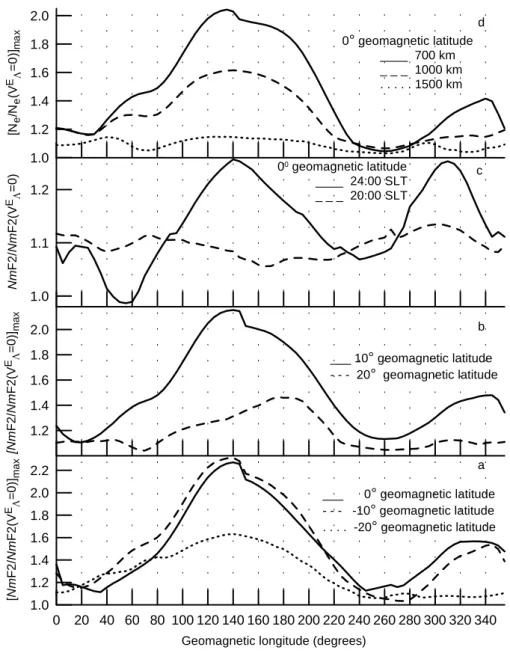
The two low panels of Fig. 7 show the maximum model value of NmF2/NmF2(VE3=0) during 12–13 April 1958 at the geomagnetic latitudes of 0◦, −10◦, −20◦ (the solid, dashed, and dotted lines in the panel (a), respectively) and 10◦, 20◦ (the solid and dashed in the panel (b), respec-tively). The longitudinal changes in the NmF2/NmF2(VE
3=0)
ratio over the geomagnetic equator at 20:00 SLT (dashed line), and 24:00 SLT (solid line) shown in the panel (d) of Fig. 6, and the maximum model value of Ne/Ne(VE3=0)
over the geomagnetic equator at 700 km (solid line), 1000 km (dashed line), and 1500 km (dotted line), shown in the top panel of Fig. 7, are discussed later in this section. The model results show that there are significant dif-ferences in [NmF2/NmF2(VE3=0)]max at different
2564 A. V. Pavlov: The role of the zonal E×B plasma drift in the low-latitude ionosphere
0 20 40 60 80 100 120 140 160 180 200 220 240 260 280 300 320 340
Geomagnetic longitude (degrees) Fig.7 1.0 1.2 1.4 1.6 1.8 2.0 2.2 [Nm F2 /Nm F2(V E Λ =0 )]max 1.2 1.4 1.6 1.8 2.0 [N m F2 /Nm F2 (V E Λ =0 )]max ___ 10° geomagnetic latitude - - - 20° geomagnetic latitude ___ 0° geomagnetic latitude - - - -10° geomagnetic latitude . . . . -20° geomagnetic latitude 1.0 1.1 1.2 Nm F2 /Nm F2(V E Λ =0) 00 geomagnetic latitude ____ 24:00 SLT _ _ _ 20:00 SLT 1.0 1.2 1.4 1.6 1.8 2.0 [N e /N e (V E Λ =0 )]ma x 0° geomagnetic latitude ____ 700 km _ _ _ 1000 km . . . 1500 km a b c d 31
Fig. 7. The maximum model value of NmF2/NmF2(VE3=0) during 12–13 April 1958 at the geomagnetic latitudes of 0◦(solid line in the panel a), −10◦(dashed line in the panel a), −20◦(dotted line in the panel a), 10◦ (solid line in the panel b), and 20◦(dashed line in the panel b). The panel (c) shows the longitudinal changes of the NmF2/NmF2(VE3=0) ratio over the geomagnetic equator at 20:00 SLT (dashed line) and 24:00 SLT (solid line) on 12 April 1958. The panel (d) shows the maximum ratio of the calculated electron density over the geomagnetic equator to that obtained when the zonal E×B drift is omitted at 700 km (solid line), 1000 km (dashed line), and 1500 km (dotted line).
[NmF2/NmF2(VE3=0)]max is estimated from the numerical
simulations to be 2.15–2.31 between −10◦and 10◦ geomag-netic latitude at 140◦geomagnetic longitude, and this main peak is less pronounced at −20◦and 20◦ geomagnetic lat-itudes, in comparison with that between −10◦ and 10◦ ge-omagnetic latitude. The [NmF2/NmF2(VE3=0)]max ratio is
found to be 1.04–1.20 at 20◦geomagnetic latitude from 0◦ to 95◦and from 220◦to 360◦geomagnetic longitude, while
[NmF2/NmF2(VE
3=0)]max=1.06–1.20 at −20
◦ geomagnetic
latitude from 0◦to 25◦and from 220◦to 360◦geomagnetic
longitude. The two low panel of Fig. 7 show that the model also produces the second peak in [NmF2/NmF2(VE3=0)]max
between −10◦and 10◦geomagnetic latitude, which is equal to 1.48–1.57 and located from 330◦ to 345◦ geomagnetic longitude. As a result, the present study provides first ev-idence that there are longitude sectors where the enhance-ments in NmF2 due to the zonal E×B plasma drift are more pronounced. A noticeable feature of the change in
NmF2/NmF2(VE
3=0)]maxin geomagnetic longitude is its
lo-cal minimums in the 1.03–1.15 range, which are formed at
A. V. Pavlov: The role of the zonal E×B plasma drift in the low-latitude ionosphere 2565
20–35◦ geomagnetic longitudes and at 245–275◦
geomag-netic longitudes between −10◦ and 10◦ geomagnetic
lati-tude. Hence, this work provides first evidence that the in-fluence of the zonal E×B plasma drift on NmF2 is less pro-nounced close to the above-mentioned geomagnetic longi-tude, where local minimums of [NmF2/NmF2(VE3=0)]max
are formed. The influence of the zonal E×B plasma drift on NmF2 is feebly marked ([NmF2/NmF2(VE3=0)]max≤1.1)
and can be neglected between 55◦ and 95◦ geomagnetic longitude, between 230◦ and 300◦ geomagnetic longitude, and from 330◦ to 350◦ geomagnetic longitude at 20◦ geo-magnetic latitude, and in the 240–355◦geomagnetic longi-tude range at −20◦ geomagnetic latitude. The difference between the calculated F2-peak altitude and that obtained when the zonal E×B drift is omitted is inessential (|hmF2–
hmF2(VE
3=0)|≤10 km) at −20
◦and at 20◦geomagnetic
lat-itude between 0◦and 105◦geomagnetic longitude and from
210◦to 360◦geomagnetic longitude. By comparing the solid
and dashed lines in Fig. 2, it is seen that the night-time eastward drift over the geomagnetic equator is considerably larger than the night-time eastward drift over Arecibo. As a result of this weakening of the night-time eastward drift in geomagnetic latitude, the influence of the zonal E×B plasma drift on NmF2 and hmF2 is found to be negligible above about 25◦ and below about −26◦ geomagnetic latitude at all geomagnetic longitudes ([NmF2/NmF2(VE3=0)]max≤1.09
and |hmF2–hmF2(VE3=0)|≤5 km at −26◦and 25◦ geomag-netic latitude).
After sunset, the daytime F2-region decay is caused by O+(4S) ion losses with a rate in chemical reactions of O+(4S) ions with vibrationally unexcited and excited N
2and
O2. Field-aligned diffusion of ions and electrons transport
ionization from the topside ionosphere to F2-region altitudes maintaining night-time NmF2. The night-time gain of ion-ization at the F2-peak is caused by the meridional E×B drift, which is directed from higher L-shells to lower L-shells. The plasma drift along magnetic field lines due to neutral winds modulates the night-time NmF2 in a constructive or destruc-tive manner, depending upon the direction of the meridional wind. A poleward meridional wind causes a lowering of the F2-region height and a resulting reduction in NmF2 due to an increase in the loss rate of O+(4S) ions, whereas a meridional wind, which is equatorwards, tends to increase the value of NmF2 by transporting the plasma up along field lines to regions of lower chemical loss of O+(4S) ions. These processes lead to a dependence of NmF2 on SLT by night, forming NmF2 changes in geomagnetic longitude at fixed values of altitude and geomagnetic latitude. In addition to the above-mentioned processes, the plasma moves in longi-tude by the strong eastward zonal E×B drift velocity, cre-ating an additional source of electron and ions, so that the night-time plasma density is maintained above values which would be calculated in the absence of this eastward drift and the above-mentioned processes can modulate the effect of the zonal E×B drift on Ne. If the meridional E×B plasma drift
at 0◦geomagnetic longitude and zero neutral wind are
em-ployed at all geomagnetic longitudes, and a centered dipole approximation for the geomagnetic field (the Earth’s cen-tric tilted magnetic dipole moment is inclined with respect to the Earth’s rotational axis) is used, then the model pro-duces feebly marked variations of [NmF2/NmF2(VE3=0)]max
in geomagnetic longitude. For example, if 3=0–360◦, then [NmF2/NmF2(VE3=0)]max=1.90–2.05 over the geomagnetic
equator, and [NmF2/NmF2(VE3=0)]max=1.88–2.00 and 1.90–
1.97 at −15◦and 15◦geomagnetic latitude, respectively. As a result of the model simulations, three major causes of the calculated longitude variations in [NmF2/NmF2(VE3=0)]max
were revealed: (1) the longitudinal asymmetry in B (the ec-centric magnetic dipole is displaced from the Earth’s center and the Earth’s eccentric tilted magnetic dipole moment is inclined with respect to the Earth’s rotational axis), (2) the variations of the wind induced plasma drift in geomagnetic longitude caused by the changes in the displacement of the geomagnetic and geographic equators and the magnetic dec-lination angle in geomagnetic longitude, and (3) the varia-tions of the meridional E×B plasma drift in geomagnetic longitude (due to the longitudinal dependence of the merid-ional equatorial E×B plasma drift produced by the empirical model of Scherliess and Fejer, 1999).
In the topside night-time ionosphere, an increase in Ne
caused by the zonal E×B plasma drift is transported from lower to higher altitudes by plasma diffusion along magnetic field lines, and, simultaneously, this increase in Ne is
redis-tributed between magnetic field lines by the meridional E×B drift. As a result, the altitude dependence of the influence of VE3 on Ne in the topside ionosphere over the
geomag-netic equator is a function of changes in the effect of VE3on
NmF2 and hmF2 in geomagnetic latitude. As the top panel of
Fig. 7 shows, the maximum effect of VE3on Nedecreases in
altitude in the night-time topside ionosphere above 700 km over the geomagnetic equator and this effect is not signif-icant above about 1500 km. The model simulations show that at 1000 km altitude the maximum Ne/Ne(VE3=0) ratio
is changed between 1.07 and 1.46 at −10◦and 10◦ geomag-netic latitude and is found to be negligible at −20◦and 20◦ geomagnetic latitude.
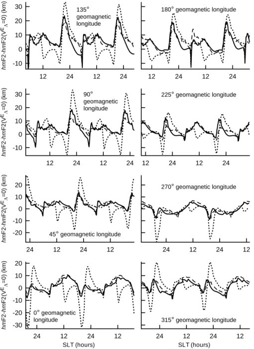
Shown in Figs. 8, 9, and 10 are plots of solar local time variations of the modeled values of NmF2/NmF2(VE3=0),
hmF2–hmF2(VE3=0), and N−e1∂3∂ Ne at hmF2 over the
geo-magnetic latitude of −15◦(solid lines), 0◦(dotted lines), and 15◦(dashed lines) at the geomagnetic longitude of 0◦, 45◦, 90◦, 135◦, 180◦, 225◦, 270◦, and 315◦.
It follows from the model simulations that 0.96≤NmF2/NmF2(VE3=0)≤1.1 from about 07:55 SLT to about 19:47 SLT over the geomagnetic equator at all geomagnetic longitudes, and from about 08:32 SLT to about 22:00 SLT at −10◦ and 10◦ geomagnetic latitude at all geomagnetic longitudes. Thus, the enhancements in NmF2 caused by the zonal E×B plasma drift are pronounced during
2566 A. V. Pavlov: The role of the zonal E×B plasma drift in the low-latitude ionosphere 24 12 24 12 1.0 1.1 1.2 1.3 Nm F2 /Nm F2(V E Λ =0) 24 12 24 12 SLT (hours) 1.0 1.2 1.4 Nm F2 /Nm F2 (V E Λ =0 ) 12 24 12 24 1.0 1.5 2.0 Nm F2 /Nm F2 (V E Λ =0 ) 12 24 12 24 1.0 1.2 1.4 1.6 Nm F2 /Nm F2 (V E Λ =0 ) 135° geomagnetic longitude 45° geomagnetic longitude 90° geomagnetic longitude 0° geomagnetic longitude 24 12 24 12 24 12 24 12 SLT (hours) 12 24 12 24 12 24 12 24 Fig. 8 180° geomagnetic longitude 270° geomagnetic longitude 315° geomagnetic longitude 225° geomagnetic longitude 32
Fig. 8. The modeled NmF2/NmF2(VE3=0) ratio as a function of SLT from 00:00 UT on 12 April 1958 to 24:00 UT on 13 April 1958 over the geomagnetic latitude of −15◦(solid lines), 0◦(dotted lines), and 15◦(dashed lines) at the geomagnetic longitudes of 0◦, 45◦, 90◦, 135◦, 180◦, 225◦, 270◦, and 315◦.
a part of the night-time period, and changes in NmF2 due to the zonal E×B plasma drift are hardly distinguished by day. As Fig. 9 shows, the difference between the calculated F2-peak altitude and that obtained when the zonal E×B drift is omitted is not significant in the daytime low-latitude ionosphere.
There are distinguishing features in the diurnal variations of N−e1∂3∂ Ne at hmF2 presented in Fig. 10. These
varia-tions show a morning maximum caused by a sharp increase in NmF2 after sunrise. During most of the daytime period
the meridional E×B drift lifts the plasma from lower field lines to higher field lines, while during most of the night-time period this drift moves ions and electrons from higher field lines to lower field lines. Simultaneously, the plasma diffuses along the magnetic field lines. As a result of the morning reversal of the meridional E×B plasma drift, ions and electrons begin to move from lower shells to higher L-shells under the action of this drift, causing a drop in NmF2 around the geomagnetic equator and a gain in ionization at F2-peak altitudes at higher geomagnetic latitudes, leading
A. V. Pavlov: The role of the zonal E×B plasma drift in the low-latitude ionosphere 2567 24 12 24 12 -20 -10 0 10 20 hm F2-hm F2(V E Λ =0) ( k m) 24 12 24 12 SLT (hours) -30 -20 -10 0 10 20 hm F2 -hm F2 (V E Λ =0 ) (km ) 12 24 12 24 -10 0 10 20 30 hm F2 -hm F2 (V E Λ =0 ) (km ) 12 24 12 24 -10 0 10 20 30 hm F2 -hm F2 (V E Λ =0 ) (km ) 135° geomagnetic longitude 45° geomagnetic longitude 90° geomagnetic longitude 0° geomagnetic longitude 24 12 24 12 24 12 24 12 SLT (hours) 12 24 12 24 12 24 12 24 Fig. 9 180° geomagnetic longitude 270° geomagnetic longitude 315° geomagnetic longitude 225° geomagnetic longitude 33
Fig. 9. The modeled hmF2–hmF2(VE3=0) difference as a function of SLT from 00:00 UT on 12 April 1958 to 24:00 UT on 13 April 1958 over the geomagnetic latitude of −15◦(solid lines), 0◦(dotted lines), and 15◦(dashed lines) at the geomagnetic longitudes of 0◦, 45◦, 90◦, 135◦, 180◦, 225◦, 270◦, and 315◦.
to the formation of the equatorial anomaly. These phys-ical processes are responsible for the formation of a local minimum in N−e1∂3∂ Ne before 12:00 SLT over the
geomag-netic equator. For the same reasons, the presence of a local evening minimum in N−e1∂3∂ Ne over the geomagnetic
equa-tor is explained by the evening pre-reversal enhancements of meridional E×B plasma drift produced by the Scherliess and Fejer (1999) model. After sunset, a decay in the day-time ionosphere leads to a decrease in NmF2 and to a de-crease in N−e1∂3∂ Ne, strengthening the influence of the zonal
E×B plasma drift on NmF2. Furthermore, Figs. 3–6 show that hmF2 makes a rapid drop in the ionosphere during most of the night-time conditions leading to an increase in the loss rate, L0, of O+(4S) ions in chemical reactions of these ions
with unexcited and vibrationally excited N2and O2at hmF2.
Thus, this night-time decrease in hmF2 leads to a strength-ening of a drop in NmF2, decreasing the value of N−e1∂3∂ Ne,
and the resulting influence of the zonal E×B plasma drift on
2568 A. V. Pavlov: The role of the zonal E×B plasma drift in the low-latitude ionosphere 24 12 24 12 -1 0 1 2 3 1 ∂ Ne Ne ∂Λ 24 12 24 12 SLT (hours) -2 -1 0 1 2 3 1 ∂ Ne Ne ∂Λ 12 24 12 24 -2 -1 0 1 2 3 1 ∂ Ne Ne ∂Λ 12 24 12 24 -1 0 1 2 3 1 ∂ Ne Ne ∂Λ 135° geomagnetic longitude 45° geomagnetic longitude 90° geomagnetic longitude 0° geomagnetic longitude 24 12 24 12 24 12 24 12 SLT (hours) 12 24 12 24 12 24 12 24 Fig. 10 180° geomagnetic longitude 270° geomagnetic longitude 315° geomagnetic longitude 225° geomagnetic longitude (ra d ian -1) (r adian -1) (radi an -1) (ra d ian -1) 34
Fig. 10. The modeled value of N−e1∂3∂ Neat hmF2 as a function of SLT from 00:00 UT on 12 April 1958 to 24:00 UT on 13 April 1958 over the geomagnetic latitude of −15◦(solid lines), 0◦(dotted lines), and 15◦(dashed lines) at the geomagnetic longitudes of 0◦, 45◦, 90◦, 135◦, 180◦, 225◦, 270◦, and 315◦.
The zonal E×B plasma drift, which is used in the model simulations, is directed from the geomagnetic west to the ge-omagnetic east by night, and the maximum eastward drift is about 165 m s−1 close to 20:45 SLT at F-region altitudes over the geomagnetic equator (see solid line in Fig. 2). Af-ter a peak before midnight, the magnitude of VE
3at F-region
altitudes over Jicamarca is observed to decrease with local time during the night-time period and during a part of the daytime period (after sunrise), reaching the minimum drift velocity at 11:15–12:15 SLT (see solid line in Fig. 2). Fig-ure 8 shows the tendency of the influence of the zonal E×B
plasma drift on NmF2 to peak close to and after midnight, i.e. the NmF2/NmF2(VE3=0) ratio peaks a few hours later than VE3. It means that the night-time dependence of NmF2 on VE3is essentially nonlocal in time, i.e. the value of NmF2 at the fixed solar local time, t1, depends on the values of VE3
from t0 to t1, where t0is a solar local time at sunset.
Fur-thermore, Fig. 10 shows that during most of the night-time period, the value of N−1
e ∂3∂ Neat hmF2 is decreased in time,
strengthening the dependence of Neon VE3. As a result, the
influence of the eastward E×B plasma drift on NmF2 is ac-cumulated and, after a small drop, this effect is strengthened
A. V. Pavlov: The role of the zonal E×B plasma drift in the low-latitude ionosphere 2569
in time up to a time point, with the following weakness of this influence. This conclusion can be illustrated from the re-duced continuity equation for O+(4S) ions, which takes into
account only the loss rate of these ions and the zonal E×B plasma drift as (only for qualitative evaluations)
∂ ∂tNe= −L0Ne+V E 3H −1N e, (6)
where H−1=−(h3Ne)−1 ∂∂3Ne, t is SLT, and it was taken into
account that [O+(4S)]≈Neat altitudes of the F2-layer.
In virtue of Eq. (6), the night-time electron density decay is described as Ne(t1, q, U, 3)=Ne(t0, q, U, 3)exp {− t1 Z t0 (L0−V3EH −1 )dt }. (7)
It is evident from Eq. (7) that NmF2(t1)depends on the
val-ues of VE3and H from t0to t1. The zonal E×B plasma drift
cannot change Ne noticeably if changes in Ne in the e3
di-rection are feebly marked. On the other hand, changes in Ne
due the zonal E×B plasma drift lead to a dependence of H on VE3. In addition to the daytime F2-region decay, during the night-time period, the meridional E×B drift moves ions and electrons from higher field lines to lower field lines, and, simultaneously, the plasma drifts due to neutral winds and diffuses along magnetic field lines, changing the magnitude of N−e1∂3∂ Neand the resulting effect of VE3on Ne.
As Fig. 2 shows, the night-time eastward drifts are consid-erably larger than the westward daytime drifts at F-region al-titudes over the geomagnetic equator. Contrary to night-time conditions, the dependence of NmF2 on VE3and N−1
e ∂3∂ Ne
cannot be illustrated by Eq. (7) and the effect of VE3on NmF2 is not accumulated in time by day during a long time period. As a result, VE3produces small effects in NmF2 during the studied daytime periods (see Figs. 3–6 and Fig. 8).
The night-time meridional E×B drift of electrons and ions moves the plasma from higher L-shells to lower L-shells and redistributes changes in electron and ion densities between field lines. Therefore, variations in Ni and Necaused by the
zonal E×B drift at magnetic field lines, which do not inter-sect the studied F-region altitudes, can lead to changes in the studied hmF2 and NmF2. It follows from the model calcula-tions that the night-time values of hmF2 and NmF2 over the magnetic equator are weakly sensitive to variations in VE3 at magnetic field lines, which cross the geomagnetic equa-tor above about the 800–900 km height. The model simula-tions show that the [NmF2/NmF2(VE3=0)]maxratio over the
geomagnetic equator at the 0–360◦ geomagnetic longitudes
is less than 1.28 and 1.47, if VE3=0 at magnetic field lines, which cross the geomagnetic equator above 500 and 600 km height, respectively. It should be noted that hmF2≤400 km from 21:54–23:08 SLT to 24:00 SLT and from 00:00 SLT to 08:07–09:34 SLT over the geomagnetic equator, if the model employs the value of VE3described in Sect. 2. As a result, the zonal E×B plasma drift at magnetic field lines, which
crosses the geomagnetic equator at F2-layer altitudes, cannot change NmF2 very noticeably by night because during most of the night-time period, electron density changes in 3 at
hmF2 at the same solar local time and geomagnetic longitude
are less pronounced over the geomagnetic equator in com-parison with those from about −10◦to about −20◦ geomag-netic latitude or between about 10◦and about 20◦ geomag-netic latitude (see Fig. 9). On the other hand, it follows from the model calculations presented by the solid line in the two lower panels of Fig. 6 that [NmF2/NmF2(VE3=0)]max ≤2.27
over the geomagnetic equator, if the value of VE3described in Sect. 2 is used. It means that the night-time dependence of NmF2 on VE3 is essentially nonlocal in space close to the geomagnetic equator.
Sterling et al. (1969) found no significant effects of VE3 on NmF2 without reporting the values of SLT and the ge-omagnetic longitudes and latitudes, where the Sterling et al. (1969) comparisons between separate calculations of Ne
with and without the zonal E×B plasma drift were carried out. Contrary to the study by Sterling et al. (1969), it is found in this work that the effect of including the zonal E×B plasma drift in the model results in the maximum increase in the night-time NmF2 up to a factor of 1.04–2.31 in the low latitude ionosphere between −20◦and 20◦geomagnetic latitude. It should be noted that there are significant differ-ences between the meridional E×B plasma drift given by the empirical model of Scherliess and Fejer (1999) and that used by Sterling et al. (1969), and these differences can de-crease the effect of VE3on Nein the model simulations
pre-sented by Sterling et al. (1969). The zonal plasma drift mea-surements given by Fejer et al. (1981, 2005); Maynard et al. (1995); Sheehan and Valladares (2004) are in disagree-ment with the zonal component of VE used by Sterling et al. (1969). For example, the zonal E×B plasma drift used by Sterling et al. (1969) is varied between 100 m s−1(close to 04:30 SLT) and −100 m s−1(close to 16:30 SLT), while the average zonal F-region plasma drift measured over Jica-marca is varied from about −50 m s−1(at 11:15–12:15 SLT) to about 165 m s−1 (close to 20:45 SLT) during equinox at high solar activity (Fejer et al., 2005). It is possible to assume that the difference between VE3used by Sterling et al. (1969) and VE3 described in Sect. 2 determines the difference or a part of the difference between the conclusion of this work and the conclusion given by Sterling et al. (1969).
Anderson (1981) has reinvestigated the effects of the zonal E×B plasma drift on the equatorial F-region ionosphere for March 1979 conditions, when the solar F10.7 cm flux was about 185 units, and has found that calculated F2-peak elec-tron densities at the magnetic equator at 20:00 LT and at 24:00 LT do not differ significantly from NmF2 obtained when the zonal E×B drift is omitted. Unfortunately, Ander-son (1981) did not report the value of the geomagnetic longi-tude, which corresponds to these model results. On the other hand, the Jicamarca meridional and zonal E×B plasma drifts were used by Anderson (1981) in the model simulations, and,