Seasonal and nightly variations of gravity-wave energy density in the middle atmosphere measured by the Purple Crow Lidar

(1)

HAL Id: hal-00318396

https://hal.archives-ouvertes.fr/hal-00318396

Submitted on 6 Nov 2007

HAL is a multi-disciplinary open access

archive for the deposit and dissemination of

sci-entific research documents, whether they are

pub-lished or not. The documents may come from

teaching and research institutions in France or

abroad, or from public or private research centers.

L’archive ouverte pluridisciplinaire HAL, est

destinée au dépôt et à la diffusion de documents

scientifiques de niveau recherche, publiés ou non,

émanant des établissements d’enseignement et de

recherche français ou étrangers, des laboratoires

publics ou privés.

Seasonal and nightly variations of gravity-wave energy

density in the middle atmosphere measured by the

Purple Crow Lidar

R. J. Sica, P. S. Argall

To cite this version:

R. J. Sica, P. S. Argall. Seasonal and nightly variations of gravity-wave energy density in the middle

atmosphere measured by the Purple Crow Lidar. Annales Geophysicae, European Geosciences Union,

2007, 25 (10), pp.2139-2145. �hal-00318396�

(2)

www.ann-geophys.net/25/2139/2007/ © European Geosciences Union 2007

Annales

Geophysicae

Seasonal and nightly variations of gravity-wave energy density in

the middle atmosphere measured by the Purple Crow Lidar

R. J. Sica and P. S. Argall

Dept. of Physics and Astronomy, The University of Western Ontario, London, Ontario, Canada

Received: 17 February 2007 – Revised: 8 August 2007 – Accepted: 10 August 2007 – Published: 6 November 2007

Abstract. The Purple Crow Lidar (PCL) is a large power-aperture product monostatic Rayleigh-Raman-Sodium-resonance-fluorescence lidar, which has been in operation at the Delaware Observatory (42.9◦N, 81.4◦W, 237 m elevation) near the campus of The University of West-ern Ontario since 1992. Kinetic-energy density has been calculated from the Rayleigh-scatter system measurements of density fluctuations at temporal-spatial scales relevant for gravity waves, e.g. soundings at 288 m height resolution and 9 min temporal resolution in the upper stratosphere and mesosphere. The seasonal averages from 10 years of measurements show in all seasons some loss of gravity-wave energy in the upper stratosphere. During the equinox periods and summer the measurements are consistent with gravity waves growing in height with little saturation, in agreement with the classic picture of the variations in the height at which gravity waves break given by Lindzen (1981). The mean values compare favourably to previous measurements when computed as nightly averages, but the high temporal-spatial resolution measurements show considerable day-to-day variability. The variability over a night is often extremely large, with typical RMS fluctuations of 50 to 100% at all heights and seasons common. These measurements imply that using a daily or nightly-averaged gravity-wave energy density in numerical models may be highly unrealistic.

Keywords. Meteorology and atmospheric dynamics

(Cli-matology; Middle atmosphere dynamics; Waves and tides)

1 Introduction

Energy is transferred in the atmosphere from long spatial-temporal scales (e.g. 100s of kilometres and days) to the smallest scales (e.g. metres and seconds) by complex

inter-Correspondence to: R. J. Sica

(sica@uwo.ca)

actions between competing physical processes. Various tech-niques have measured these processes over a limited range of spatial-temporal scales. Sophisticated numerical models have been created which can cover larger ranges of the rele-vant spatial-temporal domain, but are also limited, typically at the smaller scales. Often these models include a param-eterization of the smaller-scale gravity waves. Few seasonal measurements of gravity-wave energy distributions are avail-able, particularly in the middle atmosphere, to guide these models and in particular little is known of the variability over a day.

Gravity-wave energies can be estimated in the troposphere and lower stratosphere by various techniques including high-resolution radiosonde measurements (e.g. Allen and Vincent, 1995), radars (Nastrom and Van Zandt, 1994) and satellite-borne GPS systems (e.g. Tsuda et al., 2000). Gravity waves break and deposit energy in the middle atmosphere at al-titudes that depend on the background wind and tempera-ture structempera-ture. Since both the wind and temperatempera-ture have seasonal structure, it might be expected that the gravity-wave energy deposition might also have a seasonal depen-dence. Gravity-wave energies in the upper stratosphere and mesosphere below 75 km at middle latitudes have been mea-sured using Rayleigh-scatter lidar. Wilson et al. (1991) present a climatology of potential energy per unit mass from 2 Rayleigh-scatter lidars located in southern France. Their results highlight the geographic variability of the gravity-wave energy between 2 relatively close stations, one at the foothills of the Alps and another on the Atlantic coast, and suggest a possible variation of gravity-wave energy with sea-son. Rayleigh-scatter lidar measurements of the wave spec-trum from Tsukuba, Japan by Murayama et al. (1994) gave similar results, that is a suggestion that the gravity-wave en-ergy density is larger in the winter than in the summer in the upper stratosphere. Whiteway and Carswell (1995) saw an increase in the energy density in January relative to the rest of the year in the upper stratosphere.

(3)

2140 R. J. Sica and P. S. Argall: Variations of gravity-wave energy density in the middle atmosphere Wu and Waters (1996) estimated gravity wave variances

from microwave radiance measurements taken by the Mi-crowave Limb Sounder on the Upper Atmosphere Research Satellite. At mid-latitudes in the Northern Hemisphere they reported a factor of 2 increase in the upper stratosphere and mesospheric normalized gravity wave variance for an ap-proximately 1 month period in winter 1993 relative to a 6 week period in summer 1993. The normalized variance is related to the residual variance of their measurements when other instrumental and calibration uncertainties are re-moved from the measurements, normalized to the mean ra-diance brightness temperature, to account for the consider-able variation in wave variance between the Microwave Limb Sounder’s 6 channels (as evident in their Fig. 3).

In this study, 10 years of measurements with The Uni-versity of Western Ontario’s Purple Crow Rayleigh-scatter lidar (PCL) are used to determine the variability of the ki-netic energy density (KED) due to gravity waves in the up-per stratosphere and mesosphere up to 80 km altitude. The large power-aperture product of the PCL allows the determi-nation of the KED to be made at a higher temporal-spatial resolution than previous studies. In addition to allowing the measurements to extend to greater altitudes, this increased spatial-temporal resolution allows the variability of the KED over a given night to be determined, a critical parameter not previously estimated.

2 Methodology

The PCL is a monostatic lidar system which can simultane-ously measure both Rayleigh, Raman and sodium resonance-fluorescence backscatter. The PCL has a large power-aperture product due to the use of a high power transmitter and large aperture receiver (Sica et al., 1995). The transmit-ter is a Nd:YAG laser operating at the second harmonic, with an output energy of nominally 600 mJ/pulse at 20 Hz. The re-ceiver is a 2.65-m diameter liquid mercury mirror. The large power-aperture product allows high signal-to-noise ratio den-sity fluctuation measurements to be obtained.

The KED of each density fluctuation measurement was found in the manner detailed in Sica (1999). Briefly, the fol-lowing procedure was used. The individual relative density profiles were detrended and filtered temporally by 3 s and 5 s (Hamming, 1977). The power spectral density (PSD) was de-termined by the correlogram method, similar to that used for studies of atmospheric gravity waves by Tsuda et al. (1989). The autocorrelation function is determined out to a speci-fied lag and a window function applied to the autocorrelation. The appropriately scaled Fourier transform of the autocorre-lation is then the PSD. The spectral power was determined from the area under the correlogram formed from each den-sity fluctuation profile, with the measured photon noise floor removed from each spectrum. The limits of the integration are from the length of the data series (here 1/20 km) to the

Nyquist limit (here 1/466 m). The spectral area can then be converted into a kinetic energy, potential or total energy den-sity depending on the assumptions made.

The primary quantity used in this study is the KED, which for a monochromatic gravity wave propagating upward in the atmosphere would be conserved until the wave interacts with its surroundings and “breaks”. If equipartition of energy is assumed one can equivalently use the potential energy per unit mass, which is proportional to the KED divided by the atmospheric density. Equipartition of energy implies the sys-tem is conservative and non-rotating, as rotation causes the kinetic energy to exceed the potential energy. Rotational ef-fects on gravity waves can be assumed small for horizontal scales less than a few hundred kilometres and periods less than a few hours (Holton, 1992). Rotation will increase the kinetic energy relative to the potential energy by a factor pro-portional to the square of the horizontal wavelength and in-versely proportional to the square of the period (Gill, 1982). To maximize this difference for the PCL measurements, con-sider a gravity wave in the mesosphere with a vertical wave-length of 10 km, a horizontal wavewave-length of 900 km and a period of 320 min. For this situation, the kinetic energy ex-ceeds the potential energy by only 7%. Due to the bandwidth of the lidar vertical wavenumber spectrum (20 km) and the duration of the measurement period (4.5 to 10 h) rotational effects are small, and it is assumed that the kinetic and po-tential energy are equal.

The relative spectral power is converted to a KED using the polarization equations as described in Sica (1999). This procedure acknowledges the fact that the wave spectrum over London is typically dominated by 1 or 2 long vertical wave-length (e.g. 10 km) waves (Sica and Russell, 1999). It also avoids using temperature measurements to determine fluctu-ations. A Rayleigh-scatter lidar does not directly measure temperature, rather it measures density fluctuations. Tem-peratures are retrieved using several assumptions including knowledge of an initial pressure to “seed” the temperature retrieval, constant mean molecular mass, the Ideal Gas Law and hydrostatic equilibrium. Of these assumptions the most critical here is hydrostatic equilibrium, which may not ap-ply during passage of large-scale waves through the atmo-sphere. Unlike density fluctuations, temperature fluctuations use measurements that are correlated, in the sense that the temperature retrieved at each height depends on the measure-ments at all heights above that height, again an assumption that can break down during periods of wave activity. This situation is made worse for the measurements by the PCL, since instead of nightly-averaged temperature profiles, the time resolution of the measurements is 9 min. Hence, KED is used for this study, though conversions for all results into potential energy per unit mass are provided for comparisons with studies which use this quantity.

For this study, 146 nights from the PCL database from 1994 to 2004 passed the criteria of continuous measurements in clear sky conditions for over 4.5 h in duration. Each night

(4)

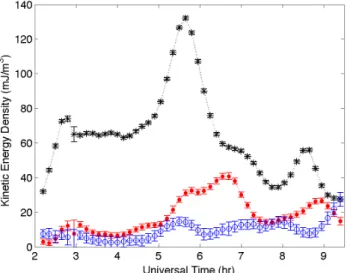
Fig. 1. Kinetic energy density as a function of time for the Low (the

upper stratosphere, 30 to 50 km; black asterisks), Middle (the lower mesosphere, 45 to 65 km; red solid circles) and High (the upper mesosphere, 60 to 80 km; blue open circles) regions on 4 Septem-ber 1994. The vertical bars are the statistical error of each mea-surement. The means of the 3 regions are Low: 64 mJ/m3, Middle: 18 mJ/m3, High: 9.3 mJ/m3. Converted to potential energy per unit mass the measurements would have means of 28, 39 and 178 J/kg, respectively.

was then divided into 3 altitude regions, Low (the upper stratosphere, 30 to 50 km), Middle (the lower mesosphere, 45 to 65 km) and High (the upper mesosphere, 60 to 80 km). To obtain reasonable errors in the measurements at the great-est heights the photocount profiles were coadded in height to 288 m and time to 9 min in each of the 3 altitude regions. The error in the energy density measurements is estimated as the fraction of the total area below the measured spectral noise floor due to photon counting statistics. Typical val-ues of the error in the energy density were ±1–3% for the Low KEDs, ±5–10% for the Middle KEDs and ±20% for the High KEDs.

3 Results

3.1 Expectations

For a monochromatic gravity wave propagating upward the kinetic energy density should be constant with height as the wave grows exponentially. If the KED decreases with height, the wave (or waves) must be giving up energy to the atmo-sphere, while if the KED increases with height the wave (or waves) are growing in amplitude more rapidly than the ez/2H growth rate for constant kinetic energy density with height (e.g. Brasseur and Solomon, 1984). Since a typical gravity wave spectrum over London contains only a few waves car-rying most of the energy, it is reasonable to assume the KED

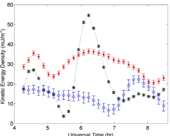
Fig. 2. Kinetic energy density on 6 April 1998 in the same

for-mat as Fig. 1. Potential energy per unit mass (J/kg) can be found by multiplying the KED by: 2.3 (Low), 0.46 (Middle) and 0.052 (High).

determinations are due to only a few dominant monochro-matic waves (Sica and Russell, 1999). This physical picture will guide us in looking at individual nights, as well as the seasonal averages.

3.2 Some representative individual nights

The temporal variability in the KED is immediately evident looking at individual night’s measurements. The selected in-dividual nights highlight the large variability in both space and time of the KED. Figure 1 shows the KEDs in the 3 height regions on the night of 4 September 1994. In Fig. 1 the vertical bars are the statistical error of the individual deter-minations of the KED. On this night, the upper stratospheric KED is large, varying by over a factor of 3 during the mea-surement period. Until approximately 06:15 UT the upper stratospheric KED is about an order of magnitude higher than the mesospheric KED. After this time the KED decreases in the upper stratosphere and lower mesosphere while the KED in the upper mesosphere remains relatively constant until af-ter 09:00, when it increases.

Figure 2 shows measurements on 6 April 1998. On this night the KED in the lower mesosphere is much larger than the upper stratosphere or lower mesosphere from 01:30 to 02:30 UT. After 03:00 UT the KED in the upper strato-sphere and lower mesostrato-sphere rapidly increases. However, from about 05:15 to 06:15 UT the KEDs are similar in all 3 regions, before the upper stratosphere KED again becomes larger.

On 15 August 1999 for the first third of the night the lower mesospheric KED is large, while the upper stratospheric KED decreases below the mesospheric values (Fig. 3). The upper stratospheric KED then increases above the

(5)

2142 R. J. Sica and P. S. Argall: Variations of gravity-wave energy density in the middle atmosphere

Fig. 3. Kinetic energy density on 15 August 1999 in the same

Figure 4. Kinetic energy density on August 17, 1994 in the same form

Fig. 4. Kinetic energy density on 17 August 1994 in the same

mesospheric values by 06:00 UT and then decreases by a factor of more than 5 times over the next hour. The lower mesospheric KED remains large the entire night.

The KED in the upper mesosphere can also be large and variable. Measurements on 17 August 1994 show the upper mesospheric KED is 5 to 10 times larger than the lower mesospheric KED for most of the measurement pe-riod (Fig. 4). The upper stratospheric KED is variable and quite large. Another example of the upper mesospheric KED being larger than the other regions is shown for 19 June 2002

Figure 5. Kinetic energy density on June 19, 2002 in the same form_{Fig. 5. Kinetic energy density on 19 June 2002 in the same}

(Fig. 5). The upper mesospheric KED is larger than the up-per stratospheric and lower mesospheric KED from 04:15 to 05:15 UT. All 3 regions have large oscillations, and the KEDs converge at around 30 mJ/m3around 07:00 UT.

3.3 Statistics, seasonal trends and variability

Table 1 lists seasonal averages of the KED, which highlight the gross features of the measurement set. The KED in the upper stratosphere is roughly constant at 30–35 mJ/m3(16– 19 J/kg potential energy per unit mass) in the autumn, winter and spring, increasing about 70% in the summer months. In the lower mesosphere the KED is largest in the winter, de-creasing about a factor of 2 in the spring, summer and au-tumn. The KED in the upper mesosphere is about the same in the spring, summer and autumn as the lower mesosphere, consistent with gravity waves growing in amplitude, which propagate into the thermosphere. However, in the winter the KED in the upper mesosphere is a factor or 2 lower than the other seasons, and considerably smaller than the winter value in the lower mesosphere. In summary, the seasonal averages are consistent in all seasons with some loss of gravity-wave energy in the upper stratosphere. During the equinox peri-ods and summer, gravity waves grow with height in agree-ment with the classic picture of the variations in the height at which gravity waves break given by Lindzen (1981).

The distribution of KEDs on individual nights for the en-tire measurement set is shown in Fig. 6. The distribution of the KED in the upper stratosphere is broader and has many more values at higher KED (above 40 mJ/m3) than in the mesosphere, where almost all the nights have mean KEDs below 40 mJ/m3. In the statistical sense, the figure

(6)

Table 1. Seasonal averages of the kinetic energy density (mJ/m3).

Upper Lower Upper stratosphere mesosphere mesosphere Winter (DJF) 34.1 24.2 5.67 Spring (MAM) 35.6 15.2 13.8 Summer (JJA) 46.9 12.0 14.8 Autumn (SON) 32.6 12.9 12.0

is consistent with saturation or breaking of gravity waves in the mesosphere. The mean values of the KEDs are 40 mJ/m3 (equivalent to a potential energy per unit mass of 22 J/kg), 14 mJ/m3 _{(30 J/kg) and 14 mJ/m}3 _{(250 J/kg) for the upper}

stratosphere, lower mesosphere and upper mesosphere re-spectively. The upper stratospheric KED measured over southern Ontario is significantly higher than previously re-ported values from other lidars such as the measurements of Murayama et al. (1994; 10 J/kg), Wilson et al. (1991; 6 J/kg) and Whiteway and Carswell (1995; 8 J/kg), though the day-to-day variability of the energy densities is similar. Mu-rayama et al. and Wilson et al. also obtained measurements in the lower mesosphere, with potential energy per unit mass of 30 J/kg and 15–20 J/kg, respectively, more similar to the PCL measurements. Only the Wilson et al. measurements extended to the upper mesosphere, with their estimates of the potential energy per unit mass being about half that of the PCL measurements (80–100 J/kg).

Of particular interest is the difference between the Purple Crow Lidar measurements and those of Whiteway and Car-swell, which were taken from stations approximately 200 km apart over different time periods (1991–1992 for the White-way and Carswell measurements as opposed to 1994–2004 in this study). The reason for the larger values of the KED mea-sured by the PCL is primarily due to the temporal resolution of the measurements. The KEDs in this study are determined from density fluctuations obtained using 9 min lidar integra-tions. The other studies used nightly mean density fluctu-ations to estimate the energy density. To check the magni-tude of this difference the KED in the upper stratosphere was computed on each night using the nightly-averaged density fluctuation. Calculating the KED in this manner decreased its value on average by a factor of 1.5. Considering the night-to-night variability, the PCL measurements are slightly higher than the nightly averages reported in previous studies, when this difference in temporal-spatial resolution is accounted for. A unique result of this study, particularly for modellers who need to parameterize the behaviour of small-scale waves, is the histogram of the nightly geophysical variability of each night, which is the standard deviation about the mean for the night (Fig. 7). The histograms are similar for the up-per stratosphere and mesosphere, with most nights showing changes of 30 to 60%, much larger than the statistical

er-Fig. 6. Histogram of the nightly-averaged kinetic energy density

for the upper stratosphere (30 to 50 km), lower mesosphere (45 to 65 km) and upper mesosphere (60 to 80 km). Many more nights have smaller kinetic energy densities in the mesosphere than in the upper stratosphere, suggesting a loss of wave energy in the strato-sphere.

Fig. 7. Histogram of the nightly deviation of the

mean-kinetic-energy density for the upper stratosphere (30 to 50 km), lower meso-sphere (45 to 65 km) and upper mesomeso-sphere (60 to 80 km). Typical variability of the kinetic energy density over a night is about 50% in both the upper stratosphere and mesosphere.

rors of the individual measurements. These measurements are certainly not consistent with the assumption of a con-stant value of the mean KED over even periods of hours. The nightly variability of the KED is as large or often larger than the seasonal variations, and often exceeds 50% of the mean nightly value.

(7)

2144 R. J. Sica and P. S. Argall: Variations of gravity-wave energy density in the middle atmosphere

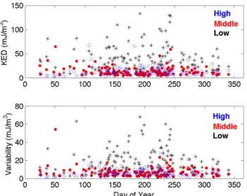
Fig. 8. The top panel shows the nightly kinetic energy density for

the composite year for the Low (the upper stratosphere, 30 to 50 km; black asterisks), Middle (the lower mesosphere, 45 to 65 km; red sold circles) and High (the upper mesosphere, 60 to 80 km; blue open circles) regions. The lower panel shows the geophysical vari-ability of the kinetic energy density during the nightly measurement period. The statistical error is negligible for the nightly average compared to the geophysical variability.

Figure 8 shows the average nightly KED and the geo-physical variability of the KED for the composite year us-ing all the available measurements in the 3 height regions. The order given by the histogram is quite different from the chaotic behaviour of the night-to-night variations. The dy-namic variations between nights (Fig. 8, top) and over a night (Fig. 8, bottom) is clearly evident. While the average sea-sonal changes are small, the variation of the wave field is extremely large. At times the variations during the night are as large as the nightly average. The fundamental result of this study is to emphasis the large variations in the gravity wave spectrum in the atmosphere on the time-scales of weather and general circulation models.

4 Conclusions

A decade of Rayleigh-scatter lidar measurements of the KED in the middle atmosphere show that seasonal variations are small compared to the variability of the KED over the night time observing period of the lidar. Previous studies have shown large day-to-day variability in the KED. PCL mea-surements have found the nightly variability on scales of hours is often 50 to 100% of the mean. The KED density typically decreases in the mesosphere relative to the upper stratosphere. This result is consistent with saturation of the gravity wave spectrum often occurring in the stratosphere. This result is also consistent with previous analysis of lidar measurements from this site that consistently show large (e.g.

a few percent) density fluctuations in the upper stratosphere. Calculating the KEDs at a resolution comparable to previous measurements of daily variations show that these measure-ments are of approximately the same magnitude, with the daily averages being about 1.5 times less than the KED de-termined at 9 min temporal resolution.

These results are important for inclusion into climate and weather models that input gravity wave energy for all, or part, of the gravity wave spectrum. The measurements obtained show it is inappropriate to use a seasonal, or often even a nightly, averaged energy density for gravity waves due to the large temporal variability. The large variability of the gravity-wave energy density could be due to modulation of wave breaking due to longer period waves such as tides or larger-scale gravity waves. Such interaction between tides and gravity waves has been shown for PCL measurements of mesospheric inversion layers (MILs) by Sica et al. (2002). Furthermore, Sica et al. (2007) have presented a theory for MILs based on the effects of large-scale waves modifying the temperature structure in which the smaller-scale waves propagate. Similar interactions may be important for the sat-uration of gravity waves and account for the variability in the measurements presented.

Acknowledgements. We would like to thank Canada’s National

Sci-ence and Engineering Council (NSERC) for provided funding for this work, as well as assistance from I. Cole and D. Turnbull in preparing the manuscript, U.-P. Hoppe and T. G. Shepherd for fruit-ful discussions concerning this work and the reviewers for their helpful comments.

Topical Editor U.-P. Hoppe thanks two anonymous referees for their help in evaluating this paper.

References

Allen, S. J. and Vincent, R. A.: Gravity-wave activity in the lower atmosphere - seasonal and latitudinal variations, J. Geophys. Res., 100, 1327–1350, 1995.

Brasseur, G. P. and Solomon, S.: Aeronomy of the Middle Atmo-sphere, Reidel, 71–80, 1984.

Gill, A. E.: Atmosphere-Ocean Dynamics, Academic Press, 266– 268, 1982.

Hamming, R. W.: Digital Filters, Prentice-Hall, 1977.

Holton, J. R.: An Introduction to Dynamic Meteorology, 3rd edi-tion, Academic Press, 206, 1992.

Lindzen, R. S.: Turbulence and stress owing to gravity wave and tidal breakdown, J. Geophys. Res., 86, 9707–9714, 1981. Murayama, Y., Tsuda, T., Wilson, R., Nakane, H., Hayashida, S. A.,

Sugimoto, N., Matsui, I., and Sasano, Y.: Gravity-wave activity in the upper-stratosphere and lower mesosphere observed with the Rayleigh lidar at Tsukuba, Japan, Geophys. Res. Lett., 21, 1539–1542, 1994.

Nastrom, G. D. and Van Zandt, T. E.: Mean vertical motions seen by radar wind profiles, J. Appl. Meteorol., 33, 984–995, 1994. Sica, R. J.: Measurements of the effects of gravity waves is the

mid-dle atmosphere using parametric models of density fluctuations.

(8)

Part II: Energy dissipation and eddy diffusion, J. Atmos. Sci., 56, 1330–1343, 1999.

Sica, R. J., Sargoytchev, S., Argall, P. S., Borra, E. F., Girard, L., Sparrow, C. T., and Flatt, S.: Lidar measurements taken with a large-aperture liquid mirror. 1. Rayleigh-scatter system, Appl. Optics, 34, 6925–6936, 1995.

Sica, R. J. and Russell, A. T.: How many waves are in the gravity wave spectrum?, Geophys. Res. Lett., 26, 3617–3620, 1999. Sica, R. J., Thayaparan, T., Argall, P. S., Russell, A. T., and

Hock-ing, W. K.: Modulation of upper mesospheric temperature in-versions due to tidal-gravity wave interactions, J. Atmos. Terr. Phys., 64, 915–922, 2002.

Sica, R. J., Argall, P. S., Shepherd, T. G., and Koshyk, J. N.: Model-measurement comparison of mesospheric temperature in-versions, and a simple theory for their occurrence, Geophys. Res. Lett., accepted, 2007.

Tsuda, T., Inoue, T., Fritts, D. C., Vanzandt, T. E., Kato, S., Sato, T., and Fukao, S.: MST radar observations of a saturated gravity-wave spectrum, J. Atmos. Sci., 46, 2440–2447, 1989.

Tsuda, T., Nishida, M., Rocken, C., and Ware, R. H.: A global morphology of gravity wave activity in the stratosphere revealed by the GPS occultation data (GPS/MET), J. Geophys. Res., 105, 7257–7273, 2000.

Whiteway, J. A. and Carswell, A. I.: Lidar observations of gravity-wave activity in the upper-stratosphere over Toronto, J. Geophys. Res., 100, 14 113–14 124, 1995.

Wilson, R., Chanin, M. L., and Hauchecorne, A.: Gravity-waves in the middle atmosphere observed by Rayleigh lidar .2. Climatol-ogy, J. Geophys. Res., 96, 5169–5183, 1991.

Wu, D. L. and Waters, J. W.: Satellite observations of atmospheric variances: A possible indication of gravity waves, Geophys. Res. Lett., 23, 3631–3634, 1996.