Publisher’s version / Version de l'éditeur:
Vous avez des questions? Nous pouvons vous aider. Pour communiquer directement avec un auteur, consultez la
première page de la revue dans laquelle son article a été publié afin de trouver ses coordonnées. Si vous n’arrivez pas à les repérer, communiquez avec nous à PublicationsArchive-ArchivesPublications@nrc-cnrc.gc.ca.
Questions? Contact the NRC Publications Archive team at
PublicationsArchive-ArchivesPublications@nrc-cnrc.gc.ca. If you wish to email the authors directly, please see the first page of the publication for their contact information.
https://publications-cnrc.canada.ca/fra/droits
L’accès à ce site Web et l’utilisation de son contenu sont assujettis aux conditions présentées dans le site LISEZ CES CONDITIONS ATTENTIVEMENT AVANT D’UTILISER CE SITE WEB.
Research Report (National Research Council of Canada. Institute for Research in
Construction), 2003-09-22
READ THESE TERMS AND CONDITIONS CAREFULLY BEFORE USING THIS WEBSITE. https://nrc-publications.canada.ca/eng/copyright
NRC Publications Archive Record / Notice des Archives des publications du CNRC :
https://nrc-publications.canada.ca/eng/view/object/?id=0f0b13a8-cd15-4265-99e2-e706951d9656 https://publications-cnrc.canada.ca/fra/voir/objet/?id=0f0b13a8-cd15-4265-99e2-e706951d9656
NRC Publications Archive
Archives des publications du CNRC
For the publisher’s version, please access the DOI link below./ Pour consulter la version de l’éditeur, utilisez le lien DOI ci-dessous.
https://doi.org/10.4224/20378803
Access and use of this website and the material on it are subject to the Terms and Conditions set forth at
Simulation of the Dynamics of the Fire for a Section of the L. H. -La
Fontaine Tunnel
Simulation of the Dynamics of the Fire for a Section of the L.H. -La
Fontaine Tunnel
Bounagui, A.; Kashef, A.; Bénichou, N.
IRC-RR-140
September 22, 2003
ABSTRACT
As part of the research project conducted at IRC to evaluate the in-place emergency ventilation strategies of the L. H. – La Fontaine tunnel, this report investigates the fire dynamics in one section of the 1.8 km long tunnel. Computer simulations of fire scenarios were carried out, using a Computational Fluid Dynamics (CFD) model to gain insight into the effect of several parameters on the fire growth, thermal conditions and species concentrations in the tunnel. A section of the tunnel was simulated to optimize the cost of computations.
In the first part of the study, a sensitivity analysis was performed to determine the effect of the computational grid size and length of the investigated section of the tunnel. The results of this analysis were used to determine the appropriate grid distribution and section length for the parametric study.
Results from the sensitive study showed that the grid size influenced both the computation time and the prediction of the temperature and smoke. The numerical model predictions show that a 300 m long section of the tunnel was sufficient to investigate the ventilation configurations.
A parametric study was conducted to investigate the effect of different ventilation configurations on fire-induced flows and conditions in the tunnel section. The parametric study indicated that when the side upper supply vents are open, higher temperatures and CO2 concentrations are observed in the evacuation path. In the roadway area, a smoke back-layering phenomenon was observed which may delay the removal of
combustion gases and heat. In addition, a higher temperature was estimated at a height of 1.5 m compared to other supply side vent scenarios. It was concluded that the
opening of the upper supply vents delayed smoke removal and, consequently, increased hazardous situations in both the traffic and escape paths.
TABLE OF CONTENTS
ABSTRACT...I TABLE OF CONTENTS...II LIST OF TABLES ...III LIST OF FIGURES... IV NOMENCLATURE ... VI 1. INTRODUCTION ...1 1.1 CFD Numerical Modeling ...1 1.2 FDS Input...2 1.2.1 Geometry ...2 1.2.2 Boundary conditions ...4 1.2.3 Fire specification ...4 1.2.4 Material properties ...4 2. SENSITIVITY ANALYSIS ...5
2.1 Grid resolution analysis...5
2.2 Section length analysis...9
3. PARAMETRIC STUDY ...12
3.1 Influence of volumetric flow rate...12
3.2 Influence of the wall vents ...17
CONCLUSIONS ...26
LIST OF TABLES
Table 1 Grid sizes and maximum temperatures ...6
Table 2 Plume centreline temperature comparaisons ...7
Table 3 Maximum temperatures for different tunnel section lengths ...10
Table 4 Volume flow rate and maximum temperatures ...12
LIST OF FIGURES
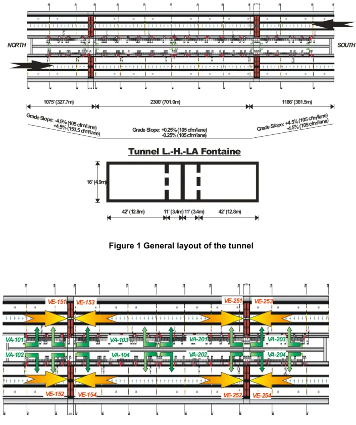
Figure 1 General layout of the tunnel ...3
Figure 2 The tunnel emergency ventilation system ...3
Figure 3 Perspective view of the tunnel section ...4
Figure 4 Comparison of the maximum temperature for all cases ...8
Figure 5 Maximum temperatures for different computation cell numbers ...8
Figure 6 Maximum temperatures for all cases ...9
Figure 7 Comparison maximum temperature for different sections- L*: non-dimensional section length: distance/section length ...11
Figure 8 Comparison maximum CO2 concentrations for different sections...11
Figure 9 Maximum temperatures for different volume flow rates...13
Figure 10 Maximum CO2 concentration for different volume flow rates ...14
Figure 11 Maximum temperatures for different volume flow rates in the escape path ...14
Figure 12 Maximum CO2 concentrations for different volume flow rate in the escape path...15
Figure 13 Iso-surface for temperature at 110°C - Vt=Ve=345 m3/s...15
Figure 14 Iso-surface for CO2 concentration at 0.006 mol/mol - Vt=Ve=345 m3/s ....16
Figure 15 Iso-surface for temperature at 170°C - Vt=Ve=115 m3/s...16
Figure 16 Iso-surface for CO2 concentrations at 0.01 mol/mol - Vt=Ve=115 m3/s ....17
Figure 17 Maximum temperatures for different vent scenarios in the escape area ...19
Figure 18 Maximum CO2 Concentration for different vent scenarios in the escape area ...19
Figure 19 Maximum temperatures in the traffic area at a height of 1.42 m...20
Figure 20 Maximum CO2 concentrations in the traffic area at a height of 1.42 m ...20
Figure 23 Iso-surface for CO2 concentrations at 0.005 (mol/mol) both side vents closed ...22 Figure 24 Iso-surface for temperature at 80°C both side vents closed...22 Figure 25 Iso-surface of temperature at 140°C lower vents closed...23
Figure 26 iso-surface CO2 concentrations at 0.009 (mol/mol) lower side vents
closed ...23 Figure 27 Iso-surface of the temperature at 110°C upper side vents closed...24
Figure 28 Iso-surface for CO2 concentrations at 0.005 (mol/mol) upper side vents
closed ...24 Figure 29 Velocity U profile for the upper vent near the fire area...25
NOMENCLATURE
*
D characteristic fire diameter (m) t
V volume flux in the traffic area of the tunnel section (m3/s)
e
V volume flux in the escape path of the tunnel section (m3/s)
.
Q total heat release rate (kW)
∞
ρ
density at ambient temperature (kg/m3) pc
specific heat of air at constant pressure (kJ/kg.K)∞
T ambient temperature (°C)
g
acceleration of gravity (m/s2)L* non-dimensional section length: distance/section length
T
cp plume centreline temperature (K)
Q
c convective heat release rate (kW) height above top of the fire source (m)z
1. INTRODUCTION
The L.-H.-La Fontaine tunnel includes a mechanical ventilation system (MVS). In the event of a fire the MVS is used to ensure the safety of the users and emergency responders.
In case of a fire in the tunnel, the operators must activate a smoke management system, which keeps the road upstream of the accident a smoke free area. This is done by keeping smoke from moving upstream and either venting it or letting it escape through the downstream portal.
When the fire department arrives on the fire scene, the operators must cooperate and modify, as needed, the smoke management system generator in order to facilitate access to the fire. At present, the standard operating procedures are based on the experience of the operators. Recently, the operating instructions were revised and formalized according to the total capacity of the MVS in venting the tunnel. However, a scientific-based validation of these operation instructions is required.
The tunnel air supply is via openings distributed along the side wall. These openings have adjustable dampers to ensure the uniformity of air distribution. They are at present completely open. It is necessary, within the framework of this project, to validate this state of opening or to propose an adjustment, compatible with the operating instructions, and optimizing the capacities of the MVS in a fire scenario.
This report investigates the fire dynamics in a section of the tunnel L. H. – La Fontaine using computer simulations. CFD numerical techniques were used to simulate the fire scenarios. The objective is to investigate the effects of ventilation configurations on the fire development, thermal conditions and species concentrations in the tunnel.
Prior to conducting the parametric study, a sensitivity analysis was performed on the computational grid resolution and the length of the tunnel section. The sensitivity analysis was used to determine the appropriate grid size and the section length that gave a good geometrically and aerodynamically representation of the tunnel at a reasonable computational cost.
The parametric study was performed to study the influence of different ventilation configurations on fire-induced flows and conditions in the selected section of the tunnel.
1.1 CFD Numerical Modeling
Fire Dynamics Simulator (FDS), a CFD fire model using large eddy simulation (LES) techniques 1 was developed by NIST. FDS has been demonstrated to predict thermal conditions resulting from a fire in an enclosure 1, 2. A CFD model requires that the enclosure of interest be divided into small rectangular control volumes or
computational cells. The CFD model computes the density, velocity, temperature, pressure and species concentrations in each control volume based on the conservation laws of mass, momentum, and energy. A complete description of the FDS model is given in reference 1.
Smokeview is a visualization program that was developed to display the results of an FDS model simulation. Smokeview produces animations or snapshots of FDS results 2.
1.2 FDS Input
FDS requires the following input:
Geometry of the tunnel being modeled, Computational cell size,
Location of the ignition source, fuel type, and heat release rate, Material thermal properties of walls, and
Boundary conditions.
1.2.1 Geometry
The L.-H.-La Fontaine tunnel, built in 1964, consists of a 1.8 km long underwater gallery in the North-South direction. The public traveller circulates on six laneways inside two concrete tubes, which are separated by a centre section. Two ventilation towers are located at the ends of the tunnel. The North tower contains a control centre that monitors the tunnel operation.
The tunnel emergency ventilation system is composed of 8 ceiling exhaust fans (4 fans for each roadway VE-151 through VE-254 ) and 8 fans (VA-101 through VA-204) that supply air through side vents uniformly distributed along one wall for each roadway in two rows. The lower and the upper side vents are located at heights of 1.0 and 3.9 m above the tunnel floor at intervals of approximately 6 m.
All fans can operate in a reverse mode. Therefore, fresh air may be supplied at either the ceiling using fans VE-151 through VE-254, or by fans VA-101 through VA-204 through the side vents. Figures 1 and 2 show the general layout of the tunnel and the emergency ventilation system. A detailed description of the tunnel is provided in reference 3.
For this study, only one section of the North roadway was simulated. The section is 300 m long, 16.2 m wide and 4.9 high. The roadway is 12.8 m wide. A 0.1 m thick concrete wall separates the traffic area from the escape area. A perspective view of the modelled section is shown in Figure 3.
1075’ (327.7m) 2300’ (701.0m) 1186’ (361.5m) Grade Slope
: -4.5% (105 cfm/lane)
+4.5% (153.5
cfm/lane) Grade Slope:
+4.5% (105 c fm/lane) -4.5% (105 c
fm/lane)
Grade Slope: +0.25% (105 cfm/lane)
-0.25% (105 cfm/lane)
SOUTH NORTH
42’ (12.8m) 11’ (3.4m)11’ (3.4m) 42’ (12.8m) 16’ (4.9m)
Tunnel L.-H.-LA Fontaine
Figure 1 General layout of the tunnel
VA-101 VA-103 VA-201 VA-203
VA-102 VA-104 VA-202 VA-204
VE-151 VE-152 VE-153 VE-154 VE-251 VE-252 VE-253 VE-254
Figure 3 Perspective view of the tunnel section
1.2.2 Boundary conditions
Two rows of supply air vents were located in the concrete wall that separates the traffic area from the escape area. The two rows vents are located respectively at
heights of 1.0 and 3.9 m above the tunnel floor and at intervals of approximately 12 m. The typical dimensions of the lower and upper vents were 1.04 m x 0.52 m and 1.4 m x 0.52 m, respectively.
Fresh air was supplied by fan VA-103 through the side vents and combustion products were exhausted by fan VE-153. Both fans were simulated as mass flow introduced or extracted at the end of the section. Therefore, at the end of the traffic area, a volume flow rate Vt of 230 m3/s was exhausted and, at the end of the escape area, a volume flow rate Ve of 230 m3/s was supplied. The ambient temperature was 20°C. The other end of the studied tunnel section was modeled as open boundary conditions.
1.2.3 Fire specification
For all simulations, a propane pool fire with a heat release rate of 15000 kW was used to represent vehicle fire. The fire area was 3 m2, 0.5 m above the tunnel floor and located at the middle of the tunnel section.
1.2.4 Material properties
The ceiling, walls, and floor of the tunnel were made of concrete with the following thermal properties:
Thermal Conductivity: 1.0 W/m.K Thermal Diffusivity: 5.7 10-7 m2/s Thickness: 0.1 m
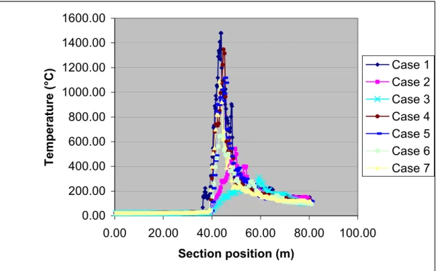
2. SENSITIVITY ANALYSIS 2.1 Grid resolution analysis
CFD numerical simulations require hours or even days to run on the latest personal computers. One of the most significant factors influencing the computation time is the size of the computational grid specified by the user. Because it is possible to over-resolve or under-resolve a space by specifying grids that are too fine or too coarse, it is important to determine an appropriate grid size for a given computational domain.
Seven grid sizes were used to study the influence of the grid size on the prediction of the temperature and the concentration of CO2 in the tunnel section. The simulations were carried out on 80 m long tunnel section. An important parameter that indicates the suitability of grid resolution is the characteristic fire diameter, D*, defined as follows: 5 2 . *
=
∞ ∞c
T
g
Q
D
pρ
where: *D
: characteristic fire diameter, m; .Q
: total heat release rate, kW;∞
ρ
: density at ambient temperature, kg/m3; pc
: specific heat of gas, kJ/kg.K;∞
T : ambient temperature, K;
g
: acceleration of gravity, m/s2;δ
∆ : grid size, m.
The ratio is an indication of the number of cells in the fire region. The higher the ratio, the better the numerical model predictions.
δ
∆
/
*
D
Another indicator is the fire resolution index which is defined as the fraction of the ideal stoichiometric value of the mixture fraction that is being used in the calculation, i. e. combustion efficiency2. It indicates how well is resolved the calculation. When the fire resolution index is equal to 1 the calculation is well resolved.
Table 1 shows the different cases along with the maximum temperatures, computation time, the maximum of ratio D*/max(∆
δ
), and the fire resolution index.Table 1 Grid sizes and maximum temperatures
Grid Size (m) x ∆
∆
y
∆
z
Grid Numbe r Total Cells Max imum Tem p erature (°C ) Run time (h) D*/max (∆δ
) Fire Resolut ion index Case 1 0.2 0.2 0.2 81x400x24 777600 1480 17.3 14 0.93 Case 2 0.4 0.4 0.4 40x200x12 96000 542 1.3 7 0.3 Case 3 0.5 0.5 0.5 30x150x9 40500 309 0.23 6 0.2 Case 4 0.4 0.4 0.1 40x200x49 392000 1347 9.8 7 1 Case 5 0.4 0.4 0.2 40x200x24 192000 1118 2.61 7 0.92 Case 6 0.4 0.6 0.2 40x135x24 129000 647 1.49 5 0.71 Case 7 0.4 0.5 0.2 40x160x24 153600 1090 1.88 6 0.82The temperatures estimated for the seven cases are shown in Figure 4. In the vicinity of the fire, the maximum temperature is higher when the grid sizes are small. The maximum temperature was underestimated when the grid size is coarse.
Figure 5 shows the maximum temperature versus computation cell numbers and Figure 6 shows the maximum temperature for all the cases. The maximum temperature increases with increasing number of control volume but the increase in temperature was limited for number of cells greater than 150,000.
The choice of the grid resolution is important for the prediction of the temperature in the fire area. Case 1 is very expensive in computation time especially for a very long tunnel section. Case 4 and Case 5 indicate that the maximum temperature improves by decreasing the grid size in the z direction (Figure 4). Since the flow is buoyancy driven,
is very influential.
z
FIERASystem Simple Correlation sub-model4 was used to calculate the plume centreline temperature and compare it to the CFD predictions. The sub-model uses Heskestad’s5 correlation to determine the plume centreline temperature and is defined as:
(
)
∞ − ∞ ∞ − + = Q z z T c g T T c p cp 3 5 0 3 2 3 1 2 . . 1 . 9ρ
where: cpT
: plume centreline temperature, K;c
Q
convective heat release rate, kW;z
height above top of the fire source, m;0
z
height of virtual origin relative to the base of fire source, m.The prediction along with the FDS models and the correlation are presented in Table 2.
Table 2 Plume centreline temperature comparaisons
FDS estimation Heskestad
estimation
Case 1 Case 2 Case 3 Case 4 Case 5 Case 6 Case 7 1721 °C 1480 °C 542 °C 309 °C 1347 °C 1118 °C 647 °C 1090 °C
The Heskestad correlation provides an estimation that is closer to Case 1 of FDS predictions. The smaller grids provide a better prediction. This mean that a better
characterization of the combustion processes and flame behaviour (Fire resolution index close to 1 Table 1). The larger grids give the worse predictions when compared to Heskestad’s correlation (Fire resolution index very low (0.2) Table 1)
From Table 1, it is observed that for values of D*/max(∆
δ
) greater than 7, the fireis well resolved (Fire resolution index close to 1). These criteria will be adopted for the parametric study, i. e., the grid cell dimensions used in case 5 will be adopted for the rest of the study.
0.00 200.00 400.00 600.00 800.00 1000.00 1200.00 1400.00 1600.00 0.00 20.00 40.00 60.00 80.00 100.00 Section position (m) Temperature (°C) Case 1 Case 2 Case 3 Case 4 Case 5 Case 6 Case 7
Figure 4 Comparison of the maximum temperature for all cases
C o m p u t a t i o n c e l l N u m b e r s 0 2 0 0 x 1 03 4 0 0 x 1 03 6 0 0 x 1 03 8 0 0 x 1 03 1 x 1 06 M a x imu m T e m pera tur e (° C) 2 0 0 4 0 0 6 0 0 8 0 0 1 0 0 0 1 2 0 0 1 4 0 0 1 6 0 0
0 200 400 600 800 1000 1200 1400 1600
Case1 Case2 Case3 Case4 Case5 Case6 Case7
Simulations
Maximum Temperature (°C)
Figure 6 Maximum temperatures for all cases
2.2 Section length analysis
Tunnels can be long and to carry out a simulation for the full length of a tunnel would be very time consuming. Assuming that the influence of the fire is negligible far from the fire, only a portion of the tunnel needs to be modelled. Consequently, the cost of the numerical computation can be reduced.
Three tunnel section lengths were used to study the influence of this parameter on the estimation of the temperatures and species concentrations. The grid from Case 5 in the previous section were used. The upper and lower vents were open.
Table 3 Maximum temperatures for different tunnel section lengths Section length (m) Maximum Temperature (°C) Maximum Temperature (°C) at the exit of the section Maximum CO2 concentration (mol/mol) Maximum CO2 concentration (mol/mol) at the exit of the
section
Case1 80 1168 116 0.12 0.0065
Case2 200 1178 84 0.12 0.0050
Case3 300 1237 27 0.12 0.0009
Figure 7 compares the temperatures estimated for the three simulations. The maximum temperature increases when the length of the tunnel section is increased. In the model, the exhaust is at the end of the tunnel section. As a result, when the length of the tunnel section is increased, the effect of the exhaust on temperature decreases. The maximum temperature at 300 m is close to the ambient temperature as shown in Table 3 and Figure 7.
Figure 8 shows similar results for the maximum concentration of the CO2.
Since the maximum of the temperature at 300 m is close to ambient temperature and the maximum of CO2 concentrations is very low at the exit of the section, a 300 m long tunnel section was chosen for the parametric study.
0 100 200 300 400 500 600 700 800 900 1000 1100 1200 1300 0 0.2 0.4 0.6 0.8 1 1. L* Temperature (°C) 2 Section 80 m Section 200 m Section 300 m
Figure 7 Comparison maximum temperature for different sections- L*: non-dimensional section length: distance/section length
0 0.02 0.04 0.06 0.08 0.1 0.12 0.14 0 0.2 0.4 0.6 0.8 1 1.2 L* CO 2 Conc e n tra tions (mol/mol) Section 80 m Section 200 m Section 300 m
3. PARAMETRIC STUDY
In case of a fire in the tunnel, the environment is modified greatly inside the tunnel. Several parameters affect the temperature level and smoke behaviour including: the volumetric flow rate, side vents, fire size and location, and traffic pattern. The
following sections will investigate the first two effects.
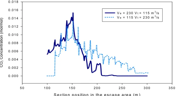
3.1 Influence of volumetric flow rate
To study the influence of the volume flow rate on the thermal distribution and species concentrations, simulation were carried out for different volumetric flow rates (Table 4). The fire was located at the middle of the tunnel.
Table 4 Volume flow rate and maximum temperatures
Maximum temperature (°C) Volume flow rate m3/s
Traffic Area Escape Area
Case 1 Vt = Ve = 115 1083 175 Case 2 Vt = Ve = 230 1237 178 Case 3 Vt = Ve = 345 1220 109 Case 4 Vt = 230, Ve = 115 1195 176 Case 5 Vt = 115, Ve = 230 1190 188 where:
Vt : volume flow rate in the traffic area Ve: volume flow rate in the escape area
Figure 9 shows the maximum temperatures in the traffic area for different sections and for different volume flow rates. The length of the high temperature decreases when the volume flow rate increases. Figure 10 shows the maximum CO2 concentrations for different sections and for different volume flow rate. The length of the high CO2 concentrations zone decreases when the volume flow rate increases. With higher volume flow rate, there is increased removal of combustion gases.
Figures 11 and 12 show the maximum temperatures and CO2 concentrations in the escape area for different sections and for two volumetric flow rates. The maximum temperature and CO2 concentration are lower for the case with the higher volume flow rate in the escape area. This can be attributed to turbulence flow in the traffic area which is caused by the high volume flow rate coming from the escape area. As a result the
From Figures 9 to 12 it was observed a similar trend for the temperature and CO2 concentrations at different section throughout the traffic area and the escape path.
Figures 13, 14, 15 and 16 show temperature and CO2 concentration iso-surfaces for Cases 1 and 2. The results indicate that the smoke layer covers a longer area when the volume flow rate in the traffic area is low.
S e c tio n p o sitio n (m ) 0 5 0 1 00 15 0 2 00 25 0 3 00 35 0 T e mp era ture (°C) 0 20 0 40 0 60 0 80 0 1 00 0 1 20 0 1 40 0 Ve = Vt = 1 15 m3/s Ve = Vt = 2 30 m 3 /s Ve = Vt = 3 4 5 m 3 /s
S e c t io n p o s it io n ( m ) 0 5 0 1 0 0 1 5 0 2 0 0 2 5 0 3 0 0 3 5 0 CO 2 c onc entrat ion (mol/mol) 0 . 0 0 0 . 0 2 0 . 0 4 0 . 0 6 0 . 0 8 0 . 1 0 0 . 1 2 0 . 1 4 Ve = Vt = 1 1 5 m3 / s Ve = Vt = 2 3 0 m3/ s Ve = Vt = 3 4 5 m3/ s
Figure 10 Maximum CO2 concentration for different volume flow rates
S e c tio n p o s itio n in th e e s c a p a r e a 5 0 1 0 0 1 5 0 2 0 0 2 5 0 3 0 0 3 5 0 Tempe ratur e ( °C ) 0 2 0 4 0 6 0 8 0 1 0 0 1 2 0 1 4 0 1 6 0 1 8 0 2 0 0 Ve = 2 3 0 Vt = 1 1 5 m3/s Ve = 1 1 5 Vt = 2 3 0 m3/s
Figure 11 Maximum temperatures for different volume flow rates in the escape path
S e c tio n p o s itio n in th e e s c a p e a r e a ( m ) 5 0 1 0 0 1 5 0 2 0 0 2 5 0 3 0 0 3 5 0 CO 2 Co nc e n tr atio n ( m o l/mo l) 0 .0 0 0 0 .0 0 2 0 .0 0 4 0 .0 0 6 0 .0 0 8 0 .0 1 0 0 .0 1 2 0 .0 1 4 0 .0 1 6 0 .0 1 8 Ve = 2 3 0 Vt = 1 1 5 m3/s Ve = 1 1 5 Vt = 2 3 0 m3/s
Figure 12 Maximum CO2 concentrations for different volume flow rate in the
escape path
Figure 16 Iso-surface for CO2 concentrations at 0.01 mol/mol - Vt=Ve=115 m3/s
3.2 Influence of the wall vents
To study the influence of the wall vents on the estimated temperatures and species concentration, simulations were conducted for different vent scenarios (Table 5). The values of the volumetric flow rate Ve and Vt are 230 m3/s. The height of 1.42 m was chosen to indicate the effect on occupants in the tunnel traffic area and the escape route.
Table 5 Case descriptions
Maximum temperature (°C) Cases Description
Traffic area Escape Area Case 1 Upper vents closed
lower vents open
1345 96
Case 2 Upper vents open lower vents closed
1112 190
Case 3 Upper and lower vents closed
1143 75
Case 4 Upper and lower vents open
Figures 17 and 18 show the maximum temperature and CO2 concentrations, respectively, in the escape path for different positions in the section of the tunnel and different vent scenarios. The maximum temperature is lower for the upper vents closed case by 100 °C. The maximum CO2 concentrations are 3 times lower for the upper vents closed case than the case with both vents open. This can be attributed to the fact that the buoyant hot smoke is restricted to enter the escape route at the upper vents.
Case 3 shows an increase in temperature above the ambient conditions although both vents are closed. This can be attributed to the conduction effect from the concrete to the escape route.
Figure 19 shows the maximum temperature in the traffic area at a height of 1.42 m for two vent scenarios (upper vents closed and both side vents open). The maximum temperature is lower by 200°C for the upper vents closed scenario than for the scenario with both the vents open. This is due to the fact that the flow from the upper vents introduces turbulence into the tunnel traffic area thus, forcing the hot smoke to move down and delaying its removal.
Figure 20 shows no impact on the CO2 concentration in the traffic area for the different vent scenarios when considering only maximum values.
Figures 21 to 26 show the iso-surface for the temperature and CO2 concentration for the four scenarios. From Figures 22 and 23, there is some effect on CO2 (better removal in case of both side vents close unlike stated in Figure 20).
For Case 4 with both side vents open and Case 2 with lower side vents closed, the hot smoke from the fire spreads symmetrically along the tunnel (Figures 21, 22, 25 and 26). The smoke layer covers a long distance in the tunnel.
A backlayering of the smoke movement was not observed for Case 3 when both side vents were closed (Figures 23 and 24). The smoke moves toward the exit.
The backlayering of the smoke was observed over a small distance for the case when the upper side vents were closed and the smoke moves toward the exit (Figures 27 and 28). With the upper side vents open, the air introduced into the traffic area forced the smoke and hot gases downwards to the tunnel floor (Figure 29) which will delay the extraction of the smoke. Thus, the backlayering of the smoke occurs when the upper side vents are open (Figure 21, 22, 25 and 26). When only the lower vents are open, minimal disturbance of the tunnel flow occurred. This led to the effective removal of hot gases and smoke.
S e c tio n p o s itio n (m ) 5 0 1 0 0 1 5 0 2 0 0 2 5 0 3 0 0 3 5 0 T e mp era ture (°C) 0 2 0 4 0 6 0 8 0 1 0 0 1 2 0 1 4 0 1 6 0 1 8 0 2 0 0 B o th v e n ts c lo s e d L o w e r v e n ts c lo s e d U p p e r v e n ts c lo s e d B o th v e n ts o p e n
Figure 17 Maximum temperatures for different vent scenarios in the escape area
S e c tio n p o s itio n (m ) 5 0 1 0 0 1 5 0 2 0 0 2 5 0 3 0 0 3 5 0 CO 2 con c en tratio n (m ol/m o l) 0 .0 0 0 0 .0 0 2 0 .0 0 4 0 .0 0 6 0 .0 0 8 0 .0 1 0 0 .0 1 2 0 .0 1 4 0 .0 1 6 L o w e r ve n ts c lo s e d U p p e r v e n ts c lo s e d B o th ve n ts o p e n
Figure 18 Maximum CO2 Concentration for different vent scenarios in the escape
S e c tio n p o s itio n (m ) 8 0 1 0 0 1 2 0 1 4 0 1 6 0 1 8 0 2 0 0 2 2 0 2 4 0 2 6 0 T e mpe ratur e ( °C ) 0 2 0 0 4 0 0 6 0 0 8 0 0 1 0 0 0 1 2 0 0 U p p e r v e n ts c lo s e d B o th v e n ts o p e n
Figure 19 Maximum temperatures in the traffic area at a height of 1.42 m
S e c tio n p o s itio n (m ) 8 0 1 0 0 1 2 0 1 4 0 1 6 0 1 8 0 2 0 0 2 2 0 2 4 0 2 6 0 CO 2 c onc e n tr atio n ( m ol/mo l) 0 .0 0 0 .0 2 0 .0 4 0 .0 6 0 .0 8 0 .1 0 0 .1 2 0 .1 4 B o th v e n ts c lo s e d L o w e r v e n ts c lo s e d U p p e r v e n ts c lo s e d B o th v e n ts o p e n
Figure 21 Iso-surface for temperature at 140°C both side vents open
Figure 23 Iso-surface for CO2 concentrations at 0.005 (mol/mol) both side vents closed
Figure 25 Iso-surface of temperature at 140°C lower vents closed
Figure 26 iso-surface CO2 concentrations at 0.009 (mol/mol) lower side vents
Figure 27 Iso-surface of the temperature at 110°C upper side vents closed
Figure 28 Iso-surface for CO2 concentrations at 0.005 (mol/mol) upper side vents
CONCLUSIONS
A CFD model, FDS, was used to perform a parametric study on different ventilation configurations for a section of the L. –H. La Fontaine tunnel. In order to determine the optimal grid distribution and tunnel section length, a sensitivity analysis was conducted.
Simulations were conducted with seven grid sizes to determine the optimal grid resolution. The numerical predictions showed that using a coarse grid resulted in an underestimation of the temperature and species concentrations. Three tunnel section lengths were investigated to determine the effect on simulation predictions. A section of 300 m in length was chosen to carry out the parametric study.
Simulations with five ventilation rates were performed to determine the effect on temperature and CO2 concentration in the tunnel section. The area of high temperature decreased in size when the ventilation rate was higher as the heat was rapidly extracted and the smoke spread was reduced.
Four ventilation scenarios were simulated to determine the effect of the side vents on fire behaviour. When the upper vents were left open, the smoke and hot gases traversed through the upper vents from the traffic area to the escape area causing higher temperature and CO2 concentrations in the escape route. Moreover in the traffic area, a high temperature was detected at a height of 1.42 m and the smoke backlayering occurred. It was also observed that the air introduced into the traffic area from the upper side vents forced the smoke and hot gases downwards to the tunnel floor.
4. REFERENCES
1. McGrattan, Kevin B., Baum, Howard R., Rehm, Ronald G., Hamins, Anthony,
Forney, Glenn P., Fire Dynamics Simulator – Technical Reference Guide,
National Institute of Standards and Technology, Gaithersburg, MD., NISTIR 6467, January 2000.
2. McGrattan, Kevin B., Forney, Glenn P., Fire Dynamics Simulator – User’s
Manual, National Institute of Standards and Technology, Gaithersburg, MD.,
NISTIR 6469, January 2000.
3. A. Kashef, N. Benichou, G. Lougheed and A. Debs. “Numerical Modeling of Air
Movement in Road Tunnels” Proceedings of the 11th Annual Conference of the CFD Society of Canada” p. 23-30, 2003.
4. P. Feng, G. V. Hadjisophocleous and D. A. Torvi, “ Equations and Theory of the
Simple Correlation Model of FIERAsystem”, Internal Report N° 779, Institue for
Research in Construction IRC, February 2000.
5. Heskestad, G., “Fire Plumes”, Chapter2-2, SPE Handbook of Fire Protection Engineering, Society of Fire Protection Engineers, Quincy, MA, USA, 1995.