Experimental procedure and uncertainty analysis of a guarded hot box method to determine the thermal transmission coefficient of skylights and sloped glazing

READ THESE TERMS AND CONDITIONS CAREFULLY BEFORE USING THIS WEBSITE. https://nrc-publications.canada.ca/eng/copyright

Vous avez des questions? Nous pouvons vous aider. Pour communiquer directement avec un auteur, consultez la

première page de la revue dans laquelle son article a été publié afin de trouver ses coordonnées. Si vous n’arrivez pas à les repérer, communiquez avec nous à PublicationsArchive-ArchivesPublications@nrc-cnrc.gc.ca.

Questions? Contact the NRC Publications Archive team at

PublicationsArchive-ArchivesPublications@nrc-cnrc.gc.ca. If you wish to email the authors directly, please see the first page of the publication for their contact information.

NRC Publications Archive

Archives des publications du CNRC

This publication could be one of several versions: author’s original, accepted manuscript or the publisher’s version. / La version de cette publication peut être l’une des suivantes : la version prépublication de l’auteur, la version acceptée du manuscrit ou la version de l’éditeur.

Access and use of this website and the material on it are subject to the Terms and Conditions set forth at

Experimental procedure and uncertainty analysis of a guarded hot box method to determine the thermal transmission coefficient of skylights and sloped glazing

Elmahdy, A. H.; Haddad, K.

https://publications-cnrc.canada.ca/fra/droits

L’accès à ce site Web et l’utilisation de son contenu sont assujettis aux conditions présentées dans le site LISEZ CES CONDITIONS ATTENTIVEMENT AVANT D’UTILISER CE SITE WEB.

NRC Publications Record / Notice d'Archives des publications de CNRC:

https://nrc-publications.canada.ca/eng/view/object/?id=66d7b11c-46f5-4c85-bcea-25a233a69c15 https://publications-cnrc.canada.ca/fra/voir/objet/?id=66d7b11c-46f5-4c85-bcea-25a233a69c15

Experimental procedure and uncertainty analysis of a guarded hotbox method to determine the thermal transmission coefficient of skylights and sloped glazing

Elmahdy, A.H.; Haddad, K.

A version of this document is published in / Une version de ce document se trouve dans : ASHRAE Transactions, v. 106, pt. 2, 2000, pp. 601-613

www.nrc.ca/irc/ircpubs

Experimental Procedure and Uncertainty Analysis of a Guarded HotBox Method to Determine the Thermal Transmission Coefficient of Skylights and Sloped Glazing

A. H. Elmahdy and K. Haddad

ABSTRACT

A laboratory test procedure and a guarded hot box facility to determine the thermal transmission coefficient of skylights are described. Skylights can be tested at an angle of inclination that can be varied from 20 to 90o off the horizontal. The experimental procedure, to determine the skylight R-value, is based on a correlation for the convective heat transfer on the warm side and the weather side of the test specimen. This correlation is obtained from calibration measurements using a calibrated transfer standard (CTS) in the inclined position. The results show that the convective heat transfer along an inclined CTS is substantially different from that along a vertical CTS. Three-dimensional simulations of the conduction heat transfer within the CTS assembly are found to be in good agreement with the experimental results. A complete error analysis for the calibration experiments and for skylight testing is presented. It is found that the experimental relative uncertainty associated with the thermal transmission coefficient of the test specimen without the frame is of the order of ±6%.

INTRODUCTION

For years, the overall thermal transmission coefficient (U-factor) of fenestration systems were determined in guarded hot box facilities, where the specimens are mounted in a vertical frame separating the two environmental chambers. Recently, the determination of the overall thermal transmission coefficient of skylights and sloped glazing at an inclined position was discussed in the research and technical communities as a requirement to assess the energy rating and labelling of this type of products.

Correlation of film heat transfer coefficient on a vertical surface in a guarded hot box environment was documented earlier in the literature [Elmahdy, 1992]. However, scarce experimental data about the variation of the film heat transfer coefficient over the surface of fenestration products in inclined position is extremely scarce. The focus of this paper is on the development of a research class guarded hot box facility to enable the accurate determination of the overall heat transfer coefficient (U-factor) of skylight and sloped glazing systems. This is in response to the needs of industry, researchers and standards writing authorities. Also, the results of this research work are critical for product certification and labelling, which is demanded by industry and building code officials.

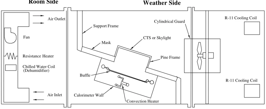
ENVIRONMENTAL TEST FACILITY

The guarded hot box facility was designed originally to test windows in the vertical position. Detailed description of this facility and the associated uncertainty analysis can be found in Elmahdy (1992). In order to accommodate the testing of skylights mounted at an angle off the horizontal, the calorimeter and the surround panel

assembly were rotated about its central axis, as shown in Figure 1. Presently, the facility can be used to test special fenestration systems with inclinations ranging from 20 to 90o off the horizontal.

A total of three fans were installed on the weather side to mix the air and to obtain the desired heat transfer coefficient on this side of the test sample, by means of changing the speed of the fan motors. On the room side, the heat was delivered through a constant temperature baffle and a convection heater. The baffle and the convection heaters are evaporating/condensing heat exchangers using refrigerant R-134a.

More details about the hot box facility can be found in Elmahdy (1992) and Brown et al. (1961).

CALIBRATION OF THE HOT-BOX

In order to use the hot box to determine the R-value of skylights, it was necessary to characterize the convection heat transfer on the room side and weather side of the specimen surface. Calibration experiments employing a Calibration Transfer Standard were carried using the hot box facility. These experiments were performed in the vertical and the inclined positions (at 20° of the horizontal). Therefore, it will be possible to test skylights in these two positions, which will help quantify the effect of the angle of inclination on the thermal resistance of a fenestration system. A total of five data sets, corresponding to five different weather side temperatures, were collected during the calibration experiments for each of the two orientations

Description of the Calibration Transfer Standard

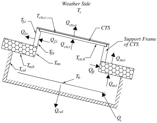
A skylight is usually installed on the outer side of the building envelope. As a result, a reentrant cavity is created between the inner side of the envelope and the warm pane of the skylight. The calibration transfer standard assembly was built with this in mind to try to duplicate as closely as possible the nature of a real skylight, as shown in Figure 2. The CTS is supported by a pine wood frame, which is used to fasten the whole assembly to the surround panel. A side view of the CTS contained inside the frame is shown in Figure 3. The total dimensions of the surface of the CTS are 1.26 m x 1.26 m, but only a 1.22 m x 1.22 m area can directly exchange heat with the warm or cold air streams due to the nature of the interface between the CTS and the frame. This smaller area is associated with the surface of the CTS glass that is in direct contact with either the warm or cold air streams on the room and weather sides, respectively. Glue was applied along all the cracks to minimize the potential of any air leakage between the weather and the room sides of the hot box assembly.

The CTS was fabricated according to the guidelines presented by Goss et al. (1991). It consists of an 11 mm thick layer of expanded polystyrene (EPS) sandwiched between two 4 mm thick clear glass panes, as shown in Figure 3. Guarded Hot plate experiments were performed on a sample of the EPS used to make the CTS to determine the variation of the thermal conductivity of the material with mean temperature. Two sets of twenty thermocouples were installed on the room side and the weather side of the

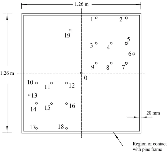
CTS. The layout of these sensors is shown in Figure 4. The temperature of each of the four sides of the frame was measured using a total of eight thermocouples, four on the room side and four on the weather side. The temperature of each of the four surround panel sides, associated with the flanking losses, was measured using a total of four thermocouples.

Initial Data Reduction Procedure

The total heat input to the calorimeter, Qt, is measured during a calibration

experiment. This heat is transferred toward the cold side of the box through several different paths. Figure 2 shows that Qt can be expressed by

) 1 ( , , ,i ctsi f i cal fl m t Q Q Q Q Q Q = + + + +

Where Qcts,i, Qm,i, and Qf,i are the heat transfers that cross the room side heat transfer

surfaces of the calibration transfer standard, the surround panel, and the support frame. The surface area of the surround panel associated with Qm,i does not include the side face

of the surround panel associated with the flanking losses Qfl. On the weather side, the

heat transfer that crosses the surfaces of the CTS, the surround panel, and the frame are designated by Qcts,o, Qm,o, and Qf,o, respectively, as shown in Figure 2. The heat transfer

through the room side surface of a certain component is not necessarily equal to that through the weather side surface of the same component due to the existence of 3-D conduction effects.

The heat transfer through the CTS is not purely 1-D in nature especially around the perimeter at the interface with the support frame. However, a good first estimate of

Qcts,i and Qcts,o is obtained from the 1-D heat conduction equation:

) 2 ( ) ( _{, ,} 1 , cts c cts h cts cts D cts R T T A Q ₋ = −

where Acts is the glass area of the CTS that directly exchanges heat with the warm air on

the room side and the cold air on the weather side. The measured thermal resistance of the expanded polystyrene inside the CTS is Rcts. The measured area-weighted averages

of the interface temperatures between the CTS core and the glass on the room side and on the weather side are designated by Tcts,h and Tcts,c, respectively. Similarly, good estimates

of the heat transfer through the frame and the surround panel, excluding the franking losses, are obtained from the 1-D conduction equation:

) 3 ( ) ( _{, ,} , 1 , f c f h f i f D f R T T A Q ₋ = − ) 4 ( ) ( _{, ,} , 1 , m c m h m o m D m R T T A Q ₋ = −

where Af,i and Am,o are the inside heat transfer area of the frame and the outside heat

transfer area of the surround panel, respectively. It is to be noted that the 1-D heat transfer estimates in Equations (2) and (3) are based on the smaller heat transfer area of each component: Af,i in the case of the frame and Am,o in the case of the surround panel.

The thermal resistance of the frame, Rf, was determined through Guarded Hot-plate

measurements, and that of the surround panel, Rm, was determined through hot box

experiments. The temperatures in Equations (3) and (4) are measured area-weighted averages of the frame and the surround panel surface temperatures on the weather side and the room side respectively.

Once the heat transfer through the CTS is determined from Equation (2), the temperatures on the outer surfaces of the room and of the weather sides of the CTS glass can be evaluated from

) 5 ( 1 , , ' , cts glass D cts h cts h cts A R Q T T = + − ) 6 ( 1 , , ' , cts glass D cts c cts c cts A R Q T T = − −

Then the heat transfer coefficients on the room and the weather sides of CTS, the support frame, and the surround panel are obtained from:

) 7 ( ) ( ) ( _' , 1 , 1 , h cts h cts D cts D i cts T T A Q h − = − − ) 8 ( ) ( ) ( _' , 1 , 1 , c c cts cts D cts D o cts T T A Q h − = − − ) 9 ( ) ( ) ( , , 1 , 1 , h f h i f D f D i f T T A Q h − = − − ) 10 ( ) ( ) ( , , 1 , 1 , c c f i f D f D o f T T A Q h − = − − ) 11 ( ) ( ) ( , , 1 , 1 , h m h o m D m D i m T T A Q h − = − − ) 12 ( ) ( ) ( , , 1 , 1 , c c m o m D m D o m T T A Q h − = − −

In reality, the heat transfers through the CTS, the frame, and the surround panel is not purely 1-D. In fact there are 3-D conduction effects especially at the interface

between the pine support frame and the CTS. The 1-D heat flow rate estimates and the associated heat transfer coefficients can be improved through 3-D conduction simulations of the heat transfer inside the calorimeter. These simulations can also be used to estimate the flanking losses through the side face of the surround panel.

Three-Dimensional Heat Transfer Simulation

The results from the heat transfer simulation are based on the assumption that there are no local variations in the heat transfer coefficient on the warm side of the CTS. In addition, a total heat transfer coefficient was used on the warm side, and the effect of separating the radiative and convective components was not carried out.

The heat transfer through the surround panel, the frame, and the CTS toward the cold side was simulated using the 3-D conduction computer program TRISCO (PHYSIBEL Inc. 1992).The grid planes employed in the simulation of the heat transfer through the surround panel, the frame, and the CTS are shown in Figure 5. Figure 5(b) is the view from the top of Figure 5(a). Due to symmetry, only one quarter of the assembly was considered. A total of nine rows, seven columns, and seven layers were employed to mark the changes in material properties and geometry. However, these planes were not enough to obtain accurate solutions of the 3-D conduction within the assembly. Additional rows, columns, and layers were defined between those shown in Figure 5. A larger number of grid planes was employed in the regions where conduction heat transfer was determined to deviate from 1-D behavior more than in the rest of the assembly. This was the case especially at the interfaces between the surround panel and the frame and the frame and CTS. The air temperatures on the weather side and the room side were specified based on the measurements from the calibration tests.

The local heat transfer coefficients were estimated using Equations (7) through (12). Adiabatic boundary conditions were used at the planes of symmetry, and at the outer edge of the surround panel. The heat transfer coefficient at the surround panel sides, associated with the flanking losses, was taken equal to that along the room side of the frame. This is deemed to be a good assumption due to the geometrical similarities between these two regions. In addition, the conduction resistance inside the surround panel dominates the total thermal resistance, from the room side to the weather side. Therefore, any minor errors in the heat transfer coefficient along the surround panel sides would have a very small effect on the predicted flanking losses.

The results of the simulations indicated a different heat flux through the inner and the outer surfaces of the CTS, the frame, and the surround panel than what was predicted using the 1-D conduction equation. These new estimates of the heat flux levels were then used to obtain better estimates of the heat transfer coefficients. The new values of the heat transfer coefficients were then used as part of the input for another TRISCO simulation. A listing of the 1-D heat transfer estimates, based on experimental temperature measurements, and those from 3-D TRISCO simulations for the inclined position are shown in Tables 1 and 2. It is to be noted that the TRISCO output provides estimates for the heat transfer through the surfaces of a specific component on the room side (Qcts,i, Qf,i, and Qm,i) and on the weather side (Qcts,o, Qf,o, and Qm,o), which are not

necessarily the same due to the existence of 3-D conduction effects. In addition, the surround panel heat transfer listed does not account for the flanking losses.

The results show that the one-dimensional estimates of the heat transfers through the CTS and the frame under predict the amount of heat that actually crosses the inner surfaces of these components, Qcts,i and Qf,i. In the case of the CTS, the 1-D heat transfer

is a good approximation of the heat that crosses the weather side surface of the calibrated transfer standard. The opposite is true in the case of the frame where the 1-D heat transfer surface is a good estimate of the heat that crosses the room side surface of the frame. The heat transfer through the cold surface of the surround panel is higher than the 1-D value due to the contribution of the flanking losses. Figure 6 shows the variation of

Qfl with the air temperature difference between the room side and the weather side.

Results for both the inclined and the vertical position are shown. As expected the flanking losses increase as the air temperature difference increases. It can also be shown that orientation has a minor effect on the flanking losses. Any differences in Qfl between

the two positions are due to differences in the inside and the outside heat transfer coefficients between the two positions. These estimates of the flanking losses are needed when performing hot box experiments with an actual skylight.

The data in Table 2 shows the measured total heat input to the calorimeter and the total heat transfer between the room side and the weather side predicted by the 3-D TRISCO simulations. There is a good agreement between the two values for the total heat input. Any discrepancy could be due to errors in the measurements of the thermal resistance of the materials of the surround panel, of the CTS, and of the frame. In addition, small leaks of cold air from the weather side could lead to a slight increase in the heat required to maintain the calorimeter at a certain temperature.

Table 3 lists heat transfer coefficients on the room side and the weather side of the CTS and the frame. The 1-D values are obtained using the measured surface temperatures and the 1-D heat conduction equation. However, the 3-D values are the refined estimates obtained using the heat fluxes from the TRISCO simulations. It is noticed that the room side heat transfer coefficients are higher along the CTS than along the frame. The airflow on the CTS resembles that of a cold plate facing downward with an unstable boundary layer. On the frame, the airflow is similar to a vertical cold flat plate with a more stable boundary layer. As the temperature driving potential on the room side increases, the total heat transfer coefficient increases as expected. The small variations in the weather side film coefficient could be attributed to changes in the cold air density with temperature and to minor changes in the RPM settings of the fans. There is more variation in the outside heat transfer of the frame probably due to the more unstable nature of this separating flow.

Convective Heat Flux Correlation for the CTS

The CTS heat flux on the room side has convection and a radiation component and it can be expressed by:

) 13 ( ) ( ) ( " , " , " ,i ctsi conv ctsi rad cts q q q = +

The warm CTS glass surface directly or indirectly exchanges heat by radiation with the frame at Tf,h, with the surround panel side at Tms, with the surround panel at Tm,h, with the

calorimeter at Tcal, and with the baffle at Tb. The baffle and the calorimeter surfaces can

be grouped together because their temperatures are very close. The equivalent surface of the calorimeter and the baffle is at a temperature Tbc. It can be shown that the radiation

heat flux component can be expressed by

) 14 ( ) ( ) ( ) ( ) ( ) ( 4 , 4 , , 4 , 4 , 4 , 4 , , 4 , 4 , " ,         − + − + − + − = h cts h f f cts h cts bc bc cts h cts h m m cts h cts ms ms cts rad i cts T T F T T F T T F T T F q σ

The appropriate radiation form factors are obtained using the computer program of Stephenson and Mitalas (1966). All the temperatures in Equation (14) are measured during a calibration test. Once the radiation component of the heat flux is found, the convection heat flux can be determined using estimates of the total heat flux on the room side of the CTS either from the 1-D conduction equation or from the TRISCO simulations.

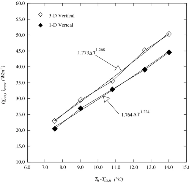
The procedure described previously was applied to the calibration data to derive correlations for the convection heat flux on the room side of the CTS for the vertical and the inclined positions. A correlation was obtained with the total CTS heat flux based on the 1-D conduction equation, and another correlation was obtained based on the total CTS heat flux from TRISCO simulations. Figures 7 and 8 show the variation of the convection CTS heat flux with the difference between the warm air temperature and the warm CTS glass surface temperature for the inclined and the vertical positions, respectively. One of the curves in each of Figures 7 and 8 is associated with the 1-D total CTS heat flux. The other curve is for the case where the total CTS heat flux is obtained from 3-D simulations. In accordance with the results listed in Table 1, the convection heat flux based on the TRISCO simulations is always higher than that based on the 1-D model for both inclinations.

The curves in Figures 7 and 8 associated with the 3-D simulations are plotted together in Figure 9 to allow for a better comparison between the vertical and the inclined positions. In the vertical position, the flow along the CTS surface is in the laminar regime based on a transition Grashof Number of 109. In this case, the average heat flux correlation is of the form A ∆T1.25 for a vertical isothermal flat plate (Incropera and Dewitt, 1985). The correlation in Figure 9 shows an exponent very similar to that reported for laminar vertical isothermal plates, which is in agreement with previous hot-box calibration experiments (Elmahdy, 1992). In the inclined position, the boundary layer becomes unstable and the convection heat transfer is higher than that in the vertical position, as shown in Figure 9.

For flow over inclined isothermal surfaces, Curcija and Goss (1995) reported the following expressions for the Grashof Number indicating the end of the laminar region:

) 15 ( 10 2 Pr) ( 94 . 2 9 θ e Gr_tr = ×

where Pr is the Prandtl Number and ? is the angle of inclination from the horizontal measured in degrees. At 20o inclination from the horizontal, this equation predicts that the transitional Grashof number is 5.5 x 106. For the calibration experiments in the inclined position, the Grashof Number was of the order of 2 x 109. Therefore, the flow over the warm CTS surface had a laminar region and a turbulent region. This is also in agreement with the reported work by Al-Arabi and Sakr (1987) . According to Al-Arabi and Sakr (1987) the average heat flux for unstable boundary layers over inclined-isothermal-flat plates can also be correlated by an expression of the form A ?TB. The exponent B is 1.25 for laminar flow and 1.333 for turbulent flow. The correlation listed in Figure 9 for the inclined position has a higher exponent than that in the case of the vertical position probably due to the occurrence of turbulent flow.

METHOD TO DETERMINE THE R-VALUE OF A SKYLIGHT

During a hot box experiment, a skylight is mounted on the surround panel as shown in Figure 10. A wood frame is used to secure the skylight to the surround panel according to the recommendations of the manufacturer. The total thermal resistance of the assembly, skylight plus frame, is the sum of the area-weighted contribution of the frame and of the skylight. In order to determine the thermal resistance of any of the two components of the assembly, it is necessary to determine the heat flow and the temperatures on the room side and on the weather side of this component.

Similar to the data reduction procedure for the calibration experiments, the heat flows within the calorimeter are related by:

) 16 ( , , ,i si f i cal fl m t Q Q Q Q Q Q = + + + +

where the total heat input, Qt, is measured during the experiment. The heat transfer

through the calorimeter wall, Qcal, is negligible equal to ±0.7 W. The flanking losses, Qfl,

and the surround panel heat transfer, Qm,i, are estimated based on the results from the

calibration experiments listed in Table 1. These results should apply as long as the conditions, temperatures and heat transfer coefficients, on the room side and the weather side of the box are the same ranges as those during the calibration experiments. The flanking losses might slightly depend on the surface temperature of the skylight employed. A different room side skylight temperature would lead to a different total heat transfer coefficient along the surround panel side associated with the flanking losses. However, this variation in the heat transfer coefficient should be small considering the limited range of room side temperatures associated with different skylights. In addition, the thermal resistances associated with the convection heat transfer on the room and weather sides are a very small fraction of that associated with conduction through the surround panel.

The heat transfer through the room side surface of the frame, Qf,i, can be

be placed on the room side and the weather side of the frame to determine the temperatures on both sides of this component. Depending on the specific geometry of the frame, the 1-D model may or may not give a good estimate of Qf,i. This method would be

more accurate for wider frames that promote 1-D heat transfer. For better accuracy, 3-D conduction simulation could be employed as it was done in the case of the calibration experiments. However, this may not be practical considering the length of time it would take to carry a test. It is to be noted also that the use of the 1-D conduction model requires an estimate of the thermal conductivity of the frame material. This information can be obtained from the literature or from separate guarded hot plate experiments.

The heat transfer through the room side of the skylight can then be determined from Equation (16). The heat flux associated with this heat flow through the skylight has a radiation and a convection component and it can be expressed by

) 17 ( ) ( ) ( "_, "_, " ,i si conv si rad s q q q = +

This skylight heat flux is based on the surface area of the skylight that exchanges heat with the room side air. The convection component of this heat flux can be expressed by an expression of the form A ?TB from Figure 9. For instance, for an inclined skylight we can write: ) 18 ( ) ( 01 . 2 ) (q_s"_{,i conv} = T_h −T_s,h 1.339

The temperature Ts,h is an estimated temperature of the warm side of the skylight, which

still needs to be determined.

Similar to the radiation heat flux of the CTS in the calibration experiments, the radiation component of the skylight heat flux on the room side can be expressed by

[

]

All the temperatures in this equation are measured during the experiment except Ts,h,

which still needs to be determined. The form factors are again determined using the program of Stephenson and Mitalas (1966). Equations (17), (18), and (19) can then be solved by iteration for an equivalent warm side temperature of the skylight Ts,h. An

) 20 ( , , " , , o s o i s i s c c s A h A q T T = +

where Tc is a measured cold side air temperature, and ho is the weather side heat transfer

coefficient determined from calibration experiments. The room side skylight heat flux has been corrected for any difference in the heat transfer area between the room side and the weather side of the skylight. Therefore, the thermal resistance of the skylight is given by: ) 21 ( ) ( , , , , i s c s h s i s s Q T T A R = − UNCERTAINTY ANALYSIS

The uncertainty levels are determined based on the method described by Moffat (1985). It is assumed that each recorded element of data is an independent observation from a Gaussian population of possible values. If R is a given function of independent variables x1, x2, …, xn, we can write

) 22 ( ) ..., , , (x₁ x₂ x_n R R=

The uncertainty associated with the result is wR and those associated with the independent

variables are w1, w2, …, wn. If these uncertainties in the independent variables have the

same odds, then the uncertainty in the result having the same odds is expressed by Kline and McLintock (1953) as ) 23 ( ... 2 / 1 2 2 2 2 2 1 1             ∂ ∂ + +     ∂ ∂ +     ∂ ∂ = _n n R w x R w x R w x R w Temperature Measurements

The temperatures were measured using a data acquisition system (DAU) and type-T thermocouples. These sensors connected to the DAU were calibrated using a water-glycol bath and a high precision Resistance-Platinum Thermometer for the range of temperatures used. The uncertainty associated with the temperature measurements was estimated to be ±0.1 oC.

Power Measurements

The total power input to the calorimeter was measured using a current shunt and a voltage divider. The DAU processed the output signal from these devices to provide the actual current and voltage for the calorimeter. These power measurements were calibrated against readings of a calibrated voltmeter and current shunts that were

traceable to primary standards. The estimated error in Qt over the range of power used

was ±0.01%.

Conductance of the CTS

The calibration transfer standard was made of a layer of expanded polystyrene (EPS) sandwiched between two layers of clear glass. The thermal resistance of the EPS was measured using the NRC Guarded Hot Plate apparatus, which is traceable to primary standards. Based on a very large number of tests, the R-value of the insulating material was estimated to within ±2%.

Uncertainty Intervals for the Calibration Experiments

The uncertainty analysis theory presented above and the uncertainties associated with the independent variables were used to estimate the error intervals for all the derived quantities. This was done for the five sets of data collected during the calibration experiments. Table 4 lists the raw experimental data and the uncertainty intervals for all the relevant derived quantities for one of these cases. It can be seen that the highest relative uncertainties are associated with the outside heat transfer coefficients of the frame and the CTS. The high heat transfer coefficients on this side of the assembly lead to lower temperature differences between the heat transfer surface and the cold air stream. As a result, the relative error associated with the temperature driving potential is higher on the weather side.

Analysis of the uncertainty of the other calibration data indicates that the relative uncertainty associated with the outside heat transfer coefficients decreases as the heat flow through the system increases. For instance, at a cold side temperature of –4 oC, the relative error associated with the outside heat transfer coefficients of the CTS is 15.2%. However, this uncertainty falls to 7.5% at a weather side air temperature of –29 oC. The relative uncertainty of the convective heat flux also decreases as the weather side air temperature decreases. It varies from 5.5% at –4 oC to 3.5% at –29 oC.

Uncertainty Intervals for Skylight Testing

Using the calibration data and uncertainties associated with the measured variables to estimate the uncertainties associated with skylight testing. It is to be noted that the calibration data applies to skylights similar to the one shown in Figure 10. In the skylight testing procedure described earlier, the heat transfer through the support frame is determined, as in the calibration experiments, from surface temperature measurements and from a prior knowledge of the thermal resistance of the frame material. Therefore, the error associated with heat transfer through the frame would be of the order of 2.2% as in the case of the calibration data. This assumes a relative uncertainty in the thermal resistance of the material of 2%, and an uncertainty of ±0.1 oC in the temperature measurements.

The other important uncertainty during skylight testing is that associated with the thermal resistance of the specimen Rs. The best estimate of the error related to Rs can

only be determined using the experimental data obtained during the testing of the specific skylight. However, a very good estimate of this uncertainty can be obtained using the calibration data and an assumed value for the total heat input Qt. During an actual

skylight testing, the flanking losses and the surround panel heat transfer would be very close to those obtained during the calibration experiment for the same room and weather side conditions. The frame heat transfer is also assumed to be equal to that obtained during calibration. From the calibration data for the inclined position for Tc = -17.5 oC,

the following heat flow rates and uncertainty intervals are obtained:

Qcal = ± 0.7 (W)

Qf,i = (38.1 ± 0.84) (W)

Qfl = (12.1 ± 0.24) (W)

Qm ,i = (37.8 ± 0.8) (W)

Using these heat transfer estimates, we can deduce that they contribute (88 ± 2.6 W) toward the total heat input to the calorimeter. If we assume a certain total heat input to the calorimeter, we can follow the procedure outlined previously to determine the thermal resistance of the skylight that would be associated with the assumed value of Qt.

The temperatures of the room side of the baffle, of the surround panel, and of the frame needed to carry this analysis are obtained from the calibration experiment for Tc = -17.5 o

C. It is expected that these temperatures would vary with the skylight tested. However, the effect of this limited change in the temperatures on the predicted relative certainty associated with Rs should be small.

The uncertainty analysis technique of Moffat (1985) can not be used to estimate the uncertainty of the warm side skylight temperature, because of the lack of a closed form expression for Ts,h. In the data reduction procedure, this temperature is solved for

by iteration using Equations (17), (18), and (19). However, these equations can be solved for the lowest or the highest possible Ts,h using the appropriate combination of the highest

or the lowest values for the variables appearing in these equations. The uncertainty analysis technique of Moffat (1985) can then be used to determine the uncertainty associated with the thermal resistance of the skylight. The resulting relevant quantities and their relative uncertainties obtained through the previous procedure are shown in Table 5. It is to be noted that the relative uncertainty, designated by R.U. in Table 5, is the ratio of the uncertainty to the absolute value of the quantity in question. The results indicate that the relative uncertainty of the heat transfer through the skylight decreases as the specimen heat transfer increases. The uncertainties in Qcal, Qf,i, Qfl, and Qm,i are

constant regardless of the total heat input. Therefore, their relative contribution toward the uncertainty of the specimen heat flow rate is smaller at higher heat flow rates.

The relative uncertainty associated with the thermal resistance of the skylight depicts an interesting trend. First it decreases as the total heat input increases. After reaching a minimum, R.U.(Rs) starts to increase with increasing values for Qt. In order to

Figure 11. The initial decrease in the relative uncertainty of Rs is due to the decrease in

the relative uncertainty of the heat transfer through the specimen. This drop in R.U.(Qs)

more than offsets the effect of the increase in R.U.(Ts,h) and R.U.(Ts,c). At a certain value

for the total heat input, the effect of the rise in the relative uncertainties of the surface temperatures of the skylight, especially Ts,h, overcomes the effect of the decrease in

R.U.(Qs).

It is to be noted also that the relative uncertainty associated with Rs listed in Table

5 is in agreement with values reported by Elmahdy (1992) in the case of window testing. In addition, some of the thermal resistance values in Table 5 should be realistic estimates for the thermal resistance of certain skylights. In fact the center glass R-value for double and triple-glazed windows, with an air gap spacing between panes of 12.7 mm, is 0.195 and 0.390 m2-K/W, respectively, as predicted by the VISION computer program from the University of Waterloo (1992). These values fall within the range of R-values included in Table 5.

CONCLUSIONS

The experimental procedure presented in this study can be employed to determine the thermal resistance of an inclined skylight similar to that considered in this paper. Based on the work performed for the purpose of the present study, the following conclusions can be made:

1) The conve ction heat transfer along the warm side of an inclined CTS is substantially higher than that along a vertical CTS. Therefore, it is very important to perform a calibration experiment at the inclination at which the skylight thermal resistance is desired.

2) There is a good agreement between the total calorimeter heat input from experiment and from three-dimensional simulation. The difference between the two values may be due to errors in the measurements of the thermal resistance of the materials. In addition any minor air leakage from the weather side to the calorimeter would increase the required heat input, and hence a higher uncertainty.

3) The flanking losses increase linearly with an increasing temperature difference between the room side and the weather side. There is very little difference between flanking losses for a vertical and for an inclined hot box.

4) The relative uncertainty of the outside heat transfer coefficient is the highest among all the relative uncertainties associated with the calibration experiments. This uncertainty decreases as the total calorimeter heat input increases.

5) The experimental relative uncertainty of the thermal resistance of a skylight is expected to be around ±6%. Initially, this uncertainty decreases as the thermal resistance of the skylight increases. After reaching a minimum, the relative uncertainty starts to increase when the skylight thermal resistance increases.

NOMENCLATURE

Acts Heat transfer area of the CTS (m2)

Af,i Heat transfer area of the room side of the frame (m2)

Af,o Heat transfer area of the weather side of the frame (m2)

Am,i Heat transfer area of the room side of the surround panel (m2)

Am,o Heat transfer area of the weather side of the surround panel (m2)

Fi,j Radiation form factor between surfaces i and j

Grt Transition Grashof Number

(hcts,i)1-D Room side heat transfer coefficient of the CTS from 1-D conduction model

(W/(m2K))

(hcts,o)1-DWeather side heat transfer coefficient of the CTS from 1-D conduction model

(W/(m2K))

(hf,i)1-D Room side heat transfer coefficient of the frame from 1-D conduction model

(W/(m2K))

(hf,o)1-D Weather side heat transfer coefficient of the frame from 1-D conduction model

(W/(m2K))

(hm,i)1-D Room side heat transfer coefficient of the surround pane l based on 1-D

conduction model (W/(m2K))

(hm,o)1-D Weather side heat transfer coefficient of the surround panel from 1-D

conduction model (W/(m2K))

Pr Prandtl Number

Qcal Heat transfer through the calorimeter wall (W)

Qcts,i Heat transfer through the room side surface of the CTS (W)

Qcts,1-D Heat transfer through the CTS based on 1-D conduction model (W)

q”cts,i Heat flux through the room side surface of the CTS (W/m2)

(qcts,i)conv Room side convection component of the CTS heat flux (W/m2)

(qcts,i)rad Room side radiation component of the CTS heat flux (W/m2)

Qf,i Heat transfer through the room side surface of the support frame (W)

Qf,o Heat transfer through the weather side surface of the support frame (W)

Qf,1-D Heat transfer through the frame based on the 1-D conduction model (W)

Qfl Flanking losses through the surround panel side (W)

Qm.i Heat transfer through the room side surface of the surround panel (W)

Qm.o Heat transfer through the weather side surface of the surround panel (W)

Qm,1-D Heat transfer through the surround panel based on the 1-D heat transfer model

(W)

Qs,i Heat transfer through the room side surface of the skylight (W)

q”s,i Total heat flux through the room side surface of the skylight (W/m2)

(q”s,i)convConvection heat transfer component on the room side surface of the skylight

(W/m2)

(q”s,i)rad Radiation heat transfer component on the room side surface of the skylight

(W/m2)

Qt Total heat input to the calorimeter (W)

Rcts Thermal resistance of the CTS core (m2K/W)

Rf Thermal resistance of the frame (m2K/W)

Rglass Thermal resistance of the CTS glass (m2K/W)

Rm Thermal resistance of the surround panel (m2K/W)

Rs Thermal resistance of the skylight (m2K/W)

Tb Baffle temperature (oC)

Tc Temperature of the air on the weather side (oC)

Tcal Calorimeter wall temperature (oC)

Tcts,c Temperature of the weather side surface of the CTS core (oC)

T’cts,c Temperature of the weather side surface of the CTS glass (oC)

Tcts,h Temperature of the room side surface of the CTS core (oC)

T’cts,h Temperature of the room side surface of the CTS glass (oC)

Tf,c Temperature of the weather side surface of the frame (oC)

Tf,h Temperature of the room side surface of the frame (oC)

Th Temperature of the air on the room side (oC)

Tm,c Temperature of the weather side surface of the surround panel (oC)

Tm,h Temperature of the room side surface of the surround panel (oC)

Tms Temperature of the surround panel side (oC)

Ts,c Temperature of the weather side surface of the skylight (oC)

Ts,h Temperature of the room side surface of the skylight (oC)

wi Uncertainty associated with xi

REFERENCES

Al-Arabi, M. and B. Sakr. 1987. Natural convection heat transfer from inclined isothermal plates. International Journal of Heat and Mass Transfer, pp. 559-565.

Brown, R.P., K.R. Solvason, and A.G. Wilson. 1961. A unique hot box cold room facility. ASHRAE Transactions 67: 561-577.

Elmahdy, A.H. 1992. Heat transmission and R-value of fenestration systems using IRC Hot Box: Procedure and uncertainty analysis. ASHRAE Transactions, Vol. 98, Part 2, 1992.

Goss, W.P., A.H. Elmahdy, and R.P. Bowen. 1990. Calibration transfer standards for fenestration systems. Proceedings of a Workshop on In-Situ Heat Flux Measurements in Buildings, Applications and Interpretations of Results. U.S. Army Cold Regions Research and Engineering Laboratory, Special Report No. 91-3.

Incorpera, F.P. and D.P. Dewitt. 1985. Fundamentals of heat transfer. John Wiley and Sons, Inc., New York.

Kline, S.J. and F.A. McClintock. 1953. Describing uncertainties in single sample experiments. Mechanical Engineering.

Moffat, R.J. 1985. Using uncertainty analysis in the planning of an experiment. Journal

of Fluids Engineering, ASME Transactions, No 107.

Mitalas, G.P., and D.G. Stephenson. 1966. Fortran IV program to calculate radiant energy interchange factors. National Research Council of Canada, Division of Building Research, Computer Program No. 25.

University of Waterloo. 1992. Vision3 glazing system thermal analysis software. Advanced Glazing System Laboratory.

PHYSIBEL, 1992. TRISCO: Computer program to calculate three-dimensional steady-state heat transfer in objects described in a beam shaped grid using the energy balance technique. Maldegem, Belgium.

Figure 1: Schematic of the NRC/IRC hot box facility for inclined skylight testing

Air Inlet Chilled Water Coil

(Dehumidifier) Resistance Heater

Fan

Air Outlet

Room Side

_{Weather Side}

R-11 Cooling Coil R-11 Cooling Coil Mask Support Frame Calorimeter Wall CTS or Skylight Cylindrical Guard Pine Frame Convection Heater Buffle

Figure 2: Details of the mounting of the CTS to the hot box and the relevant heat flows and temperatures

Q

Q

Q

Q

T

T

T

Q

Weather Side

T

T

T

T

T

T

Support Frame

of CTS

CTS

Q

Q

Q

Q

Figure 3: Details of the interface between the CTS and the support frame

40 mm

6 mm

40 mm

Clear Glass Clear Glass

4 mm

Plywood

Polystyrene

11 mm

20 mm

Figure 4: Layout of the thermocouples on the room and weather sides of the CTS

1

2

3

₄

5

7

8

9

10

11

12

14

15

16

17

18

19

6

0

20 mm 1.26 m

1.26 m

Figure 5: Rows, Columns, and Layers employed in the three-dimensional conduction simulation using TRISCO

L3 L5 L7 L9 L11 L13 L1 C1 C3 _C5C7C9 _C11 C13 Mask CTS Frame 0.040 m 0.570 m 0.610 m 0.020 m 0.197 m 1.22 m 0.006 m 0.019 m Mask Frame Flange CTS R1 R3R5_R7 R9 R11 R13 R15 R17 C1 C3 C5 C7 C9 C11 C13 0.138 m (a) (b)

Table 1: Comparison of the 1-D and the 3-D heat transfers through the CTS and the frame for the inclined position

Tc (oC) Qcts,1-D (W) 3-D Qcts,i (W) 3-D Qcts,o (W) Qf,1-D (W) 3-D Qf,i (W) 3-D Qf,o (W) -4.5 71.6 75.3 71.3 23.1 24 26.1 -11.5 89.8 93.6 88.4 29.5 30.7 33.5 -17.5 110.1 117.3 110.8 36.7 38.1 41.7 -23.4 128.9 136 128.4 43.7 45.4 49.6 -29.5 149.3 157.8 148.9 51.2 53.2 58.1

Table 2: Comparison of the 1-D and the 3-D heat transfers through the surround panel and the total heat input from experiment and from simulation

Tc (oC) Qm,1-D (W) 3-D Qm,i (W) 3-D Qm,o (W) (Qt)exp (W) (Qt)sim (W) -4.5 26.9 24.9 30.8 135.7 132.3 -11.5 33.3 30.8 38.0 169.5 165 -17.5 40.4 37.8 46.6 209.1 205.6 -23.4 47.1 43.4 53.5 246 239.2 -29.5 55.4 49.7 61.5 285.5 277.1

Table 3: Comparison of the 1-D and the 3-D heat transfer coefficients Tc (oC) (hcts,i)1-D (W/m2-K) (hcts,i)3-D (W/m2-K) (hcts,o)1-D (W/m2-K) (hcts,o)3-D (W/m2-K) (hf,i)1-D (W/m2-K) (hf,i)3-D (W/m2-K) (hf,o)1-D (W/m2-K) (hf,o)3-D (W/m2-K) -4.5 6.8 7.2 27.5 27.4 5.4 5.6 29.6 26.9 -11.5 7.1 7.4 26.5 25.8 5.7 5.8 30.7 28.1 -17.5 7.3 7.7 26 25.7 5.9 6.1 31.7 29.0 -23.4 7.4 7.7 26.5 26.2 6.1 6.2 32.8 30.3 -29.5 7.6 7.9 27.6 27.3 6.2 6.4 34.6 31.6

Figure 6: Variation of the flanking losses with the air temperature difference between the room side and the weather side

20.0 25.0 30.0 35.0 40.0 45.0 50.0 55.0 0.0 2.0 4.0 6.0 8.0 10.0 12.0 14.0 16.0 18.0 20.0 ( C)o Vertical Position Inclined Position T - T_{h c} Q (W ) fl

Figure 7: Variation of the convection heat flux on the room side of the CTS with the temperature driving potential in the inclined position

5.0 6.0 7.0 8.0 9.0 10.0 11.0 12.0 13.0 14.0 15.0 10.0 15.0 20.0 25.0 30.0 35.0 40.0 45.0 50.0 55.0 60.0 65.0 70.0 75.0 ∆T1.309 1.996 T -T ( C)o 2.01 T∆ 1.339 3-D Inclined 1-D Inclined h cts,h' (q " ) (W /m ) 2 c ts ,i c on v

Figure 8: Variation of the convection heat flux on the room side of the CTS with the temperature driving potential in the vertical position

6.0 7.0 8.0 9.0 10.0 11.0 12.0 13.0 14.0 15.0 10.0 15.0 20.0 25.0 30.0 35.0 40.0 45.0 50.0 55.0 60.0 ∆T1.224 1.764 T -T ( C)o 1.773 T∆ 1.268 3-D Vertical 1-D Vertcal h cts,h' (q " ) (W /m ) 2 c ts ,i con v

Figure 9: Comparison of the room side convection heat transfer along the CTS for the vertical and the inclined positions

6.0 7.0 8.0 9.0 10.0 11.0 12.0 13.0 14.0 15.0 10.0 15.0 20.0 25.0 30.0 35.0 40.0 45.0 50.0 55.0 60.0 65.0 70.0 75.0 ∆T1.268 1.773 T -T ( C)o (q " ) (W /m ) c ts ,i 2 2.01 T∆ 1.339 3-D Inclined 3-D Vertical h cts,h' co n v

Figure 10: Details of the mounting of the skylight to the hot box and the relevant heat flows and temperatures

Q

Q

Q

Q

T

T

T

Q

Skylight

Glazing

Weather Side at

Q

T

T

T

T

T

T

Support Frame

of Skylight

Table 4: A sample of the calibration data and the uncertainty levels associated with the measured and derived quantities

Variable Equation Quantity Absolute Uncertainty Relative Uncertainty (%) Qt Measured 169.5 0.017 W ±0.01 Th Measured 18.9 oC ±0.1 oC ±0.5 Tc Measured -11.5 oC ±0.1 oC ±0.8 Tcts,h Measured 10.3 oC ±0.1 oC ±1.0 Tcts,c Measured -8.9 oC ±0.1 oC ±1.1 Rcts Measured 0.32 m2-K/W ±0.0064 m2K/W ±2.0 Qcts,1-D Equation (2) 89.8 W ±2.01 W ±2.2 T’cts,h Equation (5) 10.5 oC ±0.1 oC ±1.0 T’cts,c Equation (6) -9.2 oC ±0.1 oC ±1.0 (hcts,i)1-D Equation (7) 7.1 W/m2-K ±0.23 W/(m2K) ±3.2 (hcts,o)1-D Equation (8) 26.5 W/m2-K 2.4 W/(m2K) ±9.0 Tf,h Measured 9.9 oC ±0.1 oC ±1.0 Tf,c Measured -9.8 oC ±0.1 oC ±1.0 Qf,1-D Equation (3) 29.5 W ±0.65 W ±2.2 (hf,i)1-D Equation (9) 5.7 W/m2-K ±0.19 W/m2-K ±3.3 (hf,o)1-D Equation (10) 30.7 W/m2-K ±3.6 W/m2-K ±11.7 Tm,h Measured 18.1 oC ±0.1 oC ±0.5 Tm,c Measured -10.8 oC ±0.1 oC ±0.9 Rm Measured 3.83 m2-K/W ±0.076 m2K/W ±2.0 Qm,1-D Equation (4) 33.3 W ±0.7 W ±2.1

(q”cts,i)rad Equation (14) 26.6 W/m2 ±0.5 W/m2 ±1.9

Table 5: Relative uncertainties associated with the data reduction procedure for skylight testing Qt (W) Qs (W) R.U.(Qs) (%) Ts,h (oC) R.U.(Ts,h) (%) Ts,c (oC) R.U.(Ts,c) Rs (m2-K/W) R.U.(Rs) (%) 150 61.94 ±6.5 13.4 ±3.8 -15.9 ±1.2 0.705 ±6.8 175 86.94 ±4.9 11.7 ±4.8 -15.3 ±1.6 0.461 ±5.4 200 111.9 ±4.0 10.0 ±6.2 -14.6 ±2.0 0.327 ±4.9 225 136.9 ±3.5 8.3 ±7.5 -14.0 ±2.5 0.242 ±4.9 250 161.9 ±3.1 6.7 ±10.8 -13.3 ±3.1 0.184 ±5.2 275 186.9 ±2.8 5.1 ±15.4 -12.7 ±3.7 0.142 ±5.8 300 211.9 ±2.6 3.6 ±23.3 -12.0 ±4.3 0.109 ±6.8

Figure 11: Variation of the relative uncertainties with the total heat input to the calorimeter 150 175 200 225 250 275 300 0 2 4 6 8 10 12 14 16 18 20 22 24 R.U.(T )_s,h R.U.(R )s _{R.U.(Q )} s R.U.(T )_s,c Q (W)_t R .U . (% )