HAL Id: hal-00271273
https://hal.archives-ouvertes.fr/hal-00271273
Preprint submitted on 8 Apr 2008
HAL is a multi-disciplinary open access
archive for the deposit and dissemination of
sci-entific research documents, whether they are
pub-lished or not. The documents may come from
teaching and research institutions in France or
abroad, or from public or private research centers.
L’archive ouverte pluridisciplinaire HAL, est
destinée au dépôt et à la diffusion de documents
scientifiques de niveau recherche, publiés ou non,
émanant des établissements d’enseignement et de
recherche français ou étrangers, des laboratoires
publics ou privés.
for System Designing and Performing Simulations
Philippe Marthon, Philippe Papaix
To cite this version:
Philippe Marthon, Philippe Papaix. SISYPHE - An Integrated Development Environment for System
Designing and Performing Simulations. 2008. �hal-00271273�
Abstract—-In order to perform simulations of complex
phenomena or solve problems, using systems is often the only resort. This paper examines the design of a general discrete-time system, modeling an interaction medium between several agents. Basic concepts like system, species, colony, subsystem, mutable arc and interface are precisely defined. An integrated development environment for system designing and performing simulations – SISYPHE – is described and some applications of system oriented programming are given.
Index Terms— Problem-solving, Simulation, System analysis
and design, System oriented programming
I. INTRODUCTION
n our world, phenomena tend to become more complex. In order to predict their evolution, simulation is often the only resort. Nevertheless, because of their complexity, the models are so approximate that their simulation significantly departs from the real evolution of the phenomenon. For example, it is the case of a meteorological phenomenon like a cyclone. It appears like indispensable to have new modeling and simulation tools at one’s disposal to design more and more complex models and perform their simulation.
II. INTERACTION AND SYSTEM
The basic idea is that a natural or artificial phenomenon is the result of an interaction: “in the beginning, was the interaction”. Interaction means a reciprocal action between two agents. In order to model interactions, the concept of system must be introduced.
A. Modeling a time-discrete system
A system (or a multi-agent system) represents a medium containing a set of agents acting on each other.
In the following, the time will be discretized and the variable t representing it, will be always an integer. So, the systems will be time-discrete systems as opposite as time-continuous systems.
P. Marthon and P. Papaïx are with the Institute of Research in Computer Science of Toulouse (IRIT), Toulouse, FRANCE (corresponding author to provide phone: +33 (0)5 61 58 83 53; fax: 33 (0)5 61 58 83 06; e-mail: Philippe.Marthon@ enseeiht.fr).
1) Agent. State of an agent. Neighborhood.
All the time, each agent m of a system is in a place k and in a state xkm (t). The places are modeled by the nodes of a graph
G (called the system graph). If an agent m1, being in a place k1,
acts on an other agent m2, being in an other place k2 the places
k1 and k2 are considered as neighbors and this relation is
modeled by an arc directed from k1 to k2 in the graph G.
In the following, we suppose that:
xkm(t) = φ (empty set) (1)
if the agent m is not in the place k at t.
2) Message or observable data
The action exercised at t, by the agent m1, being in k1, on
the agent m2, being in k2, is represented by a message dk1m1k2m2(t) (also called observable data or signal) transmitted
by the transmitter m1, circulating onto the directed arc (k1,k2),
and received by the receiver m2. This message has the effect of
modifying the state xk2m2(t) of the agent m2.
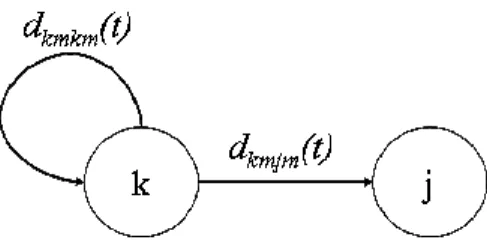
The messages can also model the moves of agents inside the graph G. So, an agent m, moving from the node k to the node j, emits two messages, one for the node k, the other for the node j. Each message describes the state of the agent m.
( )
( )
( )
( )
φ
φ
≠
=
≠
=
t
x
t
d
t
x
t
d
km kmjm km kmkm (2) At t+1, the message dkmkm(t) tells the node k that the agent mstarted from this node at t, while the message dkmjm(t) tells the
node j that this agents has just arrived in this node at t+1 (cf. fig.1.). At t+1, the states xkm and xkj are modified in this way :
( )
[
( )
(
( )
)
]
[
(
( )
)
]
( )
1
( )
(
3
b
)
)
a
3
(
!
*
*
1
t
d
t
x
t
d
t
d
t
x
t
x
kmjm jm kmkm kmkm km km=
+
=
+
==
=
+
φ
φ
φ
The rule (3a) says only that the state of the agent m in k is not modified as long as this one is staying in k while it becomes equal to φ (cf. the convention (1)) when the agent m leaves the node k.
.
SISYPHE – An Integrated Development
Environment for System Designing and
Performing Simulations
P. Marthon and P. Papaïx
Fig. 1. Sub-graph modeling the potential moving of the agent m from the node k to the node j.
3) Node state, System state
The next step of our modeling consists in giving to the nodes of G, a similar part to the agents.
So, the state xk(t) of a node k at t, is defined as the vector
composed of the states of agents being in k at t. If the system comprises P agents:
xk(t)=( xkm1(t), xkm2(t), …, xkmP(t)) (4)
The system state x(t) is defined as the vector composed of the states of all the nodes of G, at t.
x(t)=(x1(t), x2(t), …, xN(t)) (5)
where N is the number of nodes of G.
Now, the messages transmitted by the nodes can be defined. The message transmitted by the transmitter node k1 to the
receiver node k2 is the vector composed of all the messages of
different agents being in k1 at t, for the different agents which
are or can be in k2.
dk1k2(t)=( dk1m1k2(t),…, dk1mPk2(t)) (6a)
with
dk1mjk2(t)= ( dk1mjk2m1(t),…, dk1mjk2mP(t)) (6b)
Of course, it is supposed that no message is transmitted at t by the agent m from the node k if it is not in k at t:
dk1mjk2(t) = φ for all nodes k2, if the agent mj is not in k1 at t. B. Species
A species is defined as a system model. So, a species is composed of two parts:
-- a static or spatial part describing the topology of the species
-- a dynamic or temporal part describing its evolution. The spatial part is represented by a graph: its nodes represent the places where the agents are located and its arcs represent he supports of the messages transmitted by the agents.
The dynamic part is represented by rules which govern the evolutions of the states of agents and also, describe the messages exchanged by the agents.
Notice that the spatial part of a species can also evolve: some nodes and arcs can appear or disappear.
Beginning by the formal rules describing the messages, two expressions are possible:
-- either the message depends only on the node-emitter state and on the time; it corresponds to the Moore expression used to define an automaton [1]
-- or the message depends also on the messages received by the node emitter; it corresponds to the Mealy expression used to define an automaton [1]
-- Moore rule used to describe a message emitted by the agent k to the agent j
( )
t
s
(
t
x
( )
t
)
d
kj=
kj,
k (7) -- Mealy rule used to describe a message emitted by theagent k to the agent j
( )
t
s
(
t
x
( )
t
d
( )
t
d
( )
t
d
( )
t
)
d
kj=
kj,
k,
j1k,
j2k,
K
,
jpk (8)where dj1k(t), …,djpk(t) are all the messages received by the
agent k at t.
In (7) and (8), skj refers to any function.
The Mealy rule is richer than Moore’s but its application presupposes that the relation of dependence between two messages is anti-symmetric: in (8), dj1k(t), for example, does
not depend on dkj(t).
A snapshot of the environment of the node k at t, is given by the following figure 2:
Fig. 2. Snapshot of the environment of the node k at t.
Once the messages transmitted, the node states are updated according to the following rules:
( )
t
r
(
t
x
( )
t
d
( )
t
d
( )
t
d
( )
t
)
x
k+
1
=
k,
k,
j1k,
j2k,
K
,
jpk (9)where rk refers to any function.
C. Open system, Environment and Control
Generally, a system is not isolated or close but interacts with its environment. Such a system is said to be open.
Among the actions that exert their influence on a system, some of them make the system evolve to a certain direction: these actions are called controls.
D. Example
As example, consider a random walk of a mobile agent, for instance, a scarab, moving from place to place on the graph of the fig.3.
The scarab needs always one time unit to cross any arc. At each intersection of m ways, the probability that the scarab uses a path is equal to 1/m.
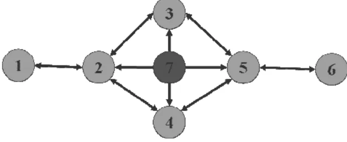
Fig. 3. Scarab’s walk system graph..
In order to guide the scarab towards a given path, a control must be applied to the node where the scarab is located. Therefore, a new node (n° 7) belonging to the environment must be introduced. This node will send a message pointing its way to the scarab. This node must be tied to the nodes having several (>1) neighbors, namely the nodes n°2, 3, 4 and 5.
Fig. 4. Scarab’s walk system graph with its environment (node 7)
To define the rules of this system, the following conventions will be used:
xk(t)=1 if the scarab agent is located in the node k at t
(k=1…6)
xk(t)=0 else
dkj(t)=1 if the scarab is present in k at t and moves on the
arc (k,j) during the interval [t,t+1]
dkj(t)=0 else Then,
( )
( )
( )1
6
1
,K
=
∀
=
+
∑
∈k
t
d
t
x
G k j jk k (10)In order to verify this last relation, notice that the scarab is present in k at t+1 only if it arrives into k at t+1 from a neighbor node. Indeed, the scarab cannot be present in k at t since it moves continuously.
For instance:
( )
t
d
( )
t
d
( )
t
d
( )
t
x
2+
1
=
12+
32+
42 (11) Computing messages is slightly more complex. It requires a random generator, called random(), taking its values in [0,1] and obeying to an uniform law. At t, the environment nodestate is equal to the result of a random drawing. This result is broadcast to all the nodes with several (m>1) neighbors.
( )
( )
( )
t
d
( )
t
d
( )
t
d
( )
t
x
( )
t
d
random
t
x
7 75 74 73 72 7=
=
=
=
=
(12) In order to simulate a random move of the scarab, the following rule must be formalized:“The scarab located in k, will take the arc (k,j) (j varying from 1 to m) if and only if the result of the random drawing, random()(ω), belongs to the interval [ j-1/m , j/m[ “
For instance, for the node n°2, the messages are:
( )
(
(
( )
)
(
( )
)
)
( )
(
(
( )
)
(
( )
)
)
( )
(
(
( )
)
(
( )
)
)
*
1
3
2
1
1
*
3
2
3
1
1
1
*
3
1
1
72 2 24 72 2 23 72 2 21t
d
et
t
x
t
d
t
d
et
t
x
t
d
t
d
et
t
x
t
d
≤
==
=
<
≤
==
=
<
==
=
(13)These three rules (13), formulated according to the Mealy syntax (8), say that the scarab located in 2, will move equally to the node 1, 3 or 4.
III. EXTENSIONS
The system model presented up to here can be improved by introducing two new concepts, the mutable arc and the subsystem.
A. Mutable arc
Until now, all messages circulate on arcs, the states of which are supposed immutable. Yet, in practice, the state of an arc is often variable and such an arc will be called a mutable arc, as opposite to an immutable arc, having a state which never varies.
Fig. 5. Mutable directed and undirected arcs
It can be noticed that a simple node can always be identified to a mutable arc with its two extremities meeting. So, the mutable arc is the basic component of any system.
Practically, the state of a mutable arc will often modify the messages crossing over this arc. So, the rules (7) and (8) must be written again as it follows:
-- Moore rule
( )
t
s
(
t
x
( ) ( )
t
w
t
)
d
kj=
kj,
k,
kj (14) -- Mealy rule( )
t
s
(
t
x
( ) ( )
t
w
t
d
( )
t
d
( )
t
d
( )
t
)
d
kj=
kj,
k,
kj,
j1k,
j2k,
K
,
jpk (15)Where wkj(t) is the state of the mutable arc (k,j) at t.
Conversely, any message dkj crossing a mutable arc (k,j),
( )
t
r
(
t
w
( ) ( )
t
d
t
)
w
kj+
1
=
kj,
kj,
kj (16) Any mutable arc, possessing a state, can transmit or receive messages as any node. It is notably the case for a visible statemutable arc, so called because its state is visible from its
initial extremity node. Indeed, such an arc (k,j) is composed of two simple arcs:
1. a mutable arc (k,j)
2. an (immutable) arc joining this mutable arc (k,j) to the initial extremity of this arc, on which a message d(k,j),k flows, transmitted by the mutable arc (k,j) and
equal to the state wkj of this arc (cf. fig. 6).
Fig. 6. Visible state mutable arc. Right, its representation in the SISYPHE environment.
In order to illustrate this new concept, consider an example derived from the road traffic: let a crossroads C to be at the intersection of three streets represented by three arcs (C,1) , (C,2) and (C,3); let it be also supposed that (C,3) is one-way and there is no entry to go from C to 3. It is appropriate for modeling the one-way street as a visible state mutable arc, the state of which is equal to “no entry”; indeed, any driver located in this crossroads C, is expected to see the no entry road sign! Notice that it is inappropriate modeling the one-way street (C,3) by an immutable arc because it would prevent physically any car to go from C to 3 whereas a visible state mutable arc does not forbid it; so, in this last case, an inattentive driver that goes the wrong way along the street (C,3), can be modeled.
Fig. 7. Modeling a crossroads. In (a), the (C,3) street is physically inaccessible : no car (message) circulates from C to 3. In (b), the street (C,3) is signposted no entry but physically accessible.
B. Subsystem
A subsystem is simply a part of a system.
A subsystem can be identified to a non-terminal node of the graph G, the state of which is the subsystem state given by (2). So, two kinds of nodes must be distinguished, terminal nodes
and non-terminal nodes (subsystems).
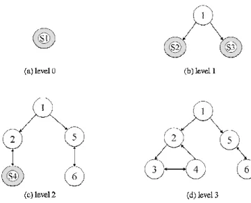
So, a system can be described hierarchically by a tree. Each node takes place in a definite level in the tree; the level number of a node is equal to its distance to the root of the tree. So, the non-terminal node representing the system is at the level 0 of the tree. The sons of the root node are at the first level, its grandsons at the second level and so on. Each level gives a possible description of the system. The higher the level number is, the more detailed is the description of the system. Notice that a non-terminal node begins to appear in a definite level of a tree and also in the other levels below it (for instance in the fig. 9, node 1 appears in the levels 1,2 and 3).
For instance, in a file system, the directories are the non-terminal nodes and the files, the non-terminal nodes.
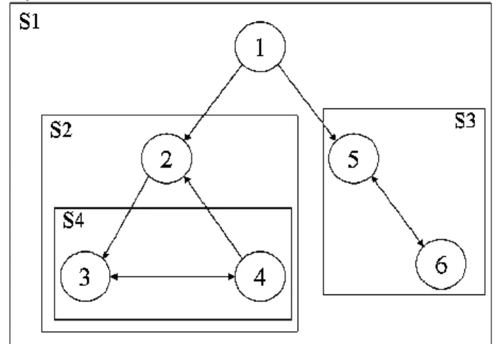
Another example is given by the system “Toto” (cf. fig. 8). S1 represents the system Toto and S2, S3 and S4 are three subsystems of S1.
Fig. 8. “Toto” system graph.
The Toto’s tree is given by the figure 9.
Fig. 9. Toto’s graph
Fig. 10. Hierarchical Toto’s description.
Taking again the scarab’s walk system, it is interesting to define the sub-graph G1, made up of nodes 1 to 6, representing the different possible paths of the walk and the subsystem S1 joined to G1.
Fig.11. Scarab walk graph. The terminal nodes are gray because they are interface nodes (cf. VI. B.)
Fig. 12. Hierarchical representation of the scarab walk.
IV. INSTANTIATING A SPECIES
Instantiating a species means to create one or several
systems from a species. All so-created systems share the same graph and the same rules.
A. Initialization
Each created system must be initialized. Initialization means to define the initial state of a system (at t = 0). If R systems have been created after instantiating, the state
( )
(
x
( ) ( )
x
x
( )
w
)
r
R
x
rNr r r r rK
K
1
)
0
(
,
0
,
,
0
,
0
0
=
1 2∀
=
must be defined (wr is the mutable arc state vector of the system n° r).
B. Colony
A colony is a group of systems of the same species sharing the same initial states.
C. Example
Taking again the scarab’s walk species, two colonies are created, each of them having one single individual. So, two scarabs S1 and S2 are created, moving across the graph of the figure 3. The initial state of each colony defines the starting point of each individual belonging to this colony. In the figure 12, the starting point of S1 (first colony) is the node 1 and the starting point of S2 (second colony) is the node 6.
V. PROGRAMMING A SPECIES
Now, in order to build any species S, a general systemic program can be given. It is supposed that S has c colonies and that each colony k consists of rk systems.
1) Build the graph G of the species S.
2) Build the rules governing the evolution of S. 3) Define the number c of colonies of S. 4) For k = 1 to c
a) Define the number rk of individuals (systems)
belonging to the kth colony b) Create these rk individuals
c) Initialize the kth colony
EndFor
VI. SYSTEM INTERACTION
Interaction is in the center of modeling natural/artificial phenomena. Nevertheless, it is quite usual to observe some independence between the different systems coexisting into the same phenomenon. So, a general simulation model must to allow systems both to evolve independently from each other and to interact from time to time.
A. General simulation model
Let a super-system S consisting of r > 1 systems, belonging or not to the same species. Let T the time between failures of S.
1) For t = 1 to T
a) Make the r systems evolved independently (in parallel)
(1) Compute (in parallel) the messages transmitted by the r systems d1(t-1), d2 (t-1),…,dr(t-1)
(2) Compute (in parallel) the new states x1(t -) , x2(t -),…, xr(t -)
b) Make the r systems interacted
(1) Compute the messages exchanged by the r systems
(2) Compute the new states x1(t) , x2(t),…, xr(t)
EndFor
B. Interface
To make the r systems interacted (previous step b.), it is necessary to define the interacting nodes.
The interface of the system S is the set of nodes able to interact with a node not belonging to S (and so, belonging to the environment of S).
Given two systems S1 and S2, let a node k1 in S1 and a node k2 in S2. These two nodes can interact if k1 belongs to the interface of S1 and k2 to the interface of S2 (necessary condition). Generally, this condition will not be sufficient (in two electronic systems, an input can be only plugged on an output and vice versa). So, the two nodes k1 and k2 can communicate only if they are “compatible”.
To define the compatibility between two interface nodes, a couple of types must be attributed to each of them. Each couple is composed of a main type and an auxiliary type.
The main type has three possible values: input (I), output (O) and input/output (I/O).
The auxiliary type is equal to a subset of the set of natural numbers.
Two nodes are said compatible if and only if the two following conditions are fulfilled: there is two couples such as
1. Either the main type value of one couple is equal to I and the other is equal to O or the two main types are equal to I/O
2. the intersection of the two auxiliary types is not empty
For instance, suppose that T1 = (E, {2,3}) is the type of a node k1 and T2 = (S, {1,2}) is the type of a node k2, then the two nodes k1 and k2 are compatible because they fulfil the two previous conditions. In the scarab walk graph of figure 11, the interface of the sub-system S1 consists of the nodes 2,3,4 and 5. the types of the interface nodes are (for instance) T2 = (E,{2}) , T3 = (E,{3}) , T4 = (E,{4}) , T5 = (E,{5}) et T7 =
(S, {2,3,4,5})
C. Example
In the previous example, two scarabs S1 and S2 have been created, moving across the graph of the figure 3. Using the SISYPHE software, a simulation of this system shows the two scarabs moving independently (cf. fig. 12).
Now, suppose that two scarabs are not indifferent to each other. More precisely, when these two scarabs meet each other, the scarab S2 will follow S1 “as its shadow”. Clearly, to get this result, the two scarab-systems must interact; so, the questions are: where and how do they interact?
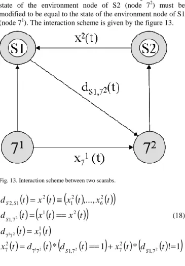
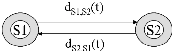
A solution is that the control conducting the scarab S2 is identical to the control of S1 after their meeting. To do it, the state of the environment node of S2 (node 72) must be modified to be equal to the state of the environment node of S1 (node 71). The interaction scheme is given by the figure 13.
Fig. 13. Interaction scheme between two scarabs.
( )
t
x
( )
t
(
x
( )
t
x
( )
t
)
d
S S 2 6 2 1 2 1 , 2=
≡
,...,
( )
t
(
x
( )
t
x
( )
t
)
d
S1,72=
1==
2 (18)( )
t
x
( )
t
d
7172=
71( )
12( )
*
(
2( )
1
)
( )
*
(
1,72( )
!
1
)
2 7 7 , 1 7 7 2 7t
=
d
t
d
t
==
+
x
t
d
t
=
x
S S VII. SIMULATIONOnce a phenomenon is modeled as a system, it can be simulated or imitated. Here, simulation means to make a system evolved by applying the general simulation model seen in VI.A.
A. Example
Taking again the scarab’s walk example, the results of a simulation are shown in the figure 14. Each scarab is represented by a square. For each node of the graph shared by the two systems, for each moment t and for each system Si
(i=1,2) , the SISYPHE simulator displays a square, the side length of which is equal to xki(t); so, no square is displayed
Fig.14. Simulation of two scarab’s walks.
VIII. SISYPHE
SISYPHE is the acronym of Simulation of Systems and Phenomena: it is also a wink at a famous character of the ancient Greek civilization. SISYPHE is an integrated development environment (IDE) for system designing and performing simulations. It allows building general-purpose systems (for instance, OPNET [2] is a specialized-purpose system, oriented on networks and telecommunications).
SISYPHE is still under development. Nevertheless, it can be used as a pedagogical tool for teaching system oriented programming.
A. Components
SISYPHE complies with the methodology of system design presented up to here. In order to build a system or a species, SISYPHE puts eight types of components – two node types and six arc types – at user’s disposal. Among them, six components can interact because they have a state, namely:
1. the subsystem node 2. the terminal node 3. the mutable (directed) arc 4. the mutable undirected arc
5. the visible state mutable (directed) arc 6. the visible state mutable undirected arc
The two other components – the (immutable directed) arc and the (immutable) undirected arc – cannot interact because they have no state. Their only function is to convey messages. Notice that all these components can be defined from one of them, namely the mutable directed arc; particularly, a terminal node can be seen as a mutable arc with the two same extremities. So, the mutable arc is the basic component of a system.
B. Species construction
In order to build and simulate a species, the following steps are required to be executed:
Step 1) Construction of the species graph G. This graph represents the topology of the species. The nodes of G can be terminal or non-terminal (subsystem). They can belong to
- The system or its environment
- The system interface or not
If a node belongs to the system interface, its type is required to be specified (cf. VI. B.). The links between nodes are directed or undirected arcs. The states of these links can be immutable, visible state mutable or invisible state mutable.
Finally, for each node, the user specifies if it will be displayed or not during the simulation.
Step 2) Construction of the rules governing the evolution of the species. The rules are logical and arithmetical phrases. Their syntax is close to Java language.
Step 3) Syntactical checking of the rules. The SISYPHE pre-compiler verifies that:
- No rule has been forgotten
- The messages obey the Mealy rule (15) - The states obey the formula (9) - The syntax of each rule is correct.
If an error appears, the user is required to come back to step 2) to correct it.
Step 4) Instantiating the species. There are two things to do:
1) Give the number of colonies and the number of
systems to create for each colony.
2) Define the initial state of each colony (and so, the initial state of each individual of the colony). The SISYPHE language syntax must be respected.
Step 5) Syntactical checking of the initialization rules. If an error appears, the user is required to come back to step 4) to correct it.
Step 6) System interaction. If a system, created in step 4), is dependent on another, the user must write the messages exchanged between these two systems and also the rules governing the evolution of the states of the interface nodes.
Step 7) Syntactical checking of the interaction rules. If an error appears, the user is required to come back to step 6) to correct it.
Step 8) Translation of the SISYPHE code into JAVA code, compilation and linkage edition. If an error appears, the user is required to come back to step 2), 4) or 6). If no error appears, an executable JAVA code is now available.
Step 9) Simulation. This simulation is achieved by the execution of the JAVA code created in step 8). The simulator displays the graph G (or a sub-graph, cf. step 1)) and the states of the displayed nodes (cf. for an example the figure 14).
IX. APPLICATIONS OF SYSTEMICS
Systemics means science of systems. Three main applications can be given.
First, it allows imitating natural or artificial phenomena and so, to predict their evolution. Notice that some researchers as Tommaso Toffoli [3] claim that cellular automata [4], a class
of time-discrete systems, are more appropriate for modeling the physical phenomena than the differential equations.
Secondly, systems can be used for problem solving (cf. X). Thirdly, computation can be easily parallelized. Actually, in a running system, each node computes in parallel with the other nodes.
For all these reasons, system-oriented programming is set to spread throughout the world of computer science.
X. PROBLEM SOLVING
Systemics is really suitable to problem solving; such problems can be found in Operations Research, Artificial Intelligence and Perception. The idea is to build a system solving a given problem. More precisely, in a systemic approach, solving a problem means
- Either define a system such as its running state x(t) is a solution of the problem
- Or define a system converging, as fast as possible, to a final state x* representing a solution of the problem.
Such a system is called optimal if it optimizes an objective function, for instance a cost or a performance. So, solving a problem for the best amounts to find an optimal system.
A. Example
This subject is illustrated with the shortest-path problem. A solution to this problem can be found by using an ant colony [5]. Indeed, an ant colony is able to discover the shortest path connecting its nest to a food depot. In order to do it, the ants deposit a chemical substance called pheromone. This matter has the effect to attract all the ants of the same species. After a time, all the ants move along the same path. This path is both the one containing the highest quantity of pheromone and the shortest path.
Using SISYPHE, a species which represents an ant colony searching a food depot can be modeled. So, it can be tested if the deposit of pheromone is sufficient to find the shortest path.
The figure 15 represents the graph of possible paths to go from the nest to food deposit.
Fig.15. Graph representing the different paths joining the nest of an ant colony to the food deposit. The nest is the node 1 and the food is the node 8.
In this model, all the basic paths are represented by visible state mutable undirected arcs. Three reasons explain this choice:
1. Along a basic path, an ant can move both ways
2. The state of each mutable undirected arc represents the whole quantity of pheromone deposited on this arc
3. The state of each arc must be visible; in actual fact, once arrived at a node, an ant is sensitive to the whole quantity deposited around this node; this fact is modeled by a message leaving each arc around the node, equal to the quantity of pheromone deposited on this arc (quantity given by the state of this arc, cf. 2.) and transmitted to the node where the ant is located.
1) Ant model
Each ant is modeled by a system. It is required that each ant 1. Moves at random
2. Moves continuously
3. Arrived at a node, is attracted by the pheromone deposited on each arc around this node; the power of attraction is proportional to the quantity deposited.
Taking again the conventions used for the scarab’s walk,
xk(t)=1 if the ant is located in the node k at t (k=1…8)
xk(t)=0 else
dkj(t)=1 if the ant is located in k at t and moves on the arc
(k,j) during the interval [t,t+1]
dkj(t)=0 else Then,
( )
( )
( )1
6
1
,K
=
∀
=
+
∑
∈k
t
d
t
x
G k j jk k (19)As it is the case for the scarab’s walk, an environment node 9 must be added to the graph G and linked to all the other nodes in order to give them the result of an uniform random drawing between 0 and 1:
( )
( )
( )
t
d
( )
t
d
( )
t
d
( )
t
x
( )
t
d
random
t
x
9 95 94 93 92 9=
=
=
=
=
(20)Now, an example of the rules governing the direction chosen by the ant is given. If the ant is located on node 4 at t (cf. fig. 15), then:
( ) ( )
(
( )
( )
(
( )
( )
( )
)
)
( ) ( )
(
( )
(
( )
( )
( )
)
)
( )
( )
( )
(
( )
( )
( )
)
(
)
( ) ( )
(
( )
( )
( )
)
(
( )
( )
( )
)
+
+
+
≥
=
+
+
+
<
≤
+
+
=
+
+
<
=
t
w
t
w
t
w
t
w
t
w
t
d
t
x
t
d
t
w
t
w
t
w
t
w
t
w
t
d
t
w
t
w
t
w
t
w
t
x
t
d
t
w
t
w
t
w
t
w
t
d
t
x
t
d
46 45 42 45 42 94 4 46 46 45 42 45 42 94 46 45 42 42 4 45 46 45 42 42 94 4 42/
*
/
/
*
/
*
(21)In these equations, to speak clearly, the states wkj(t) of the
mutable arcs (k,j) take the place of the messages d(k,j),k(t); wkj(t)
is equal to the quantity of pheromone deposited on the arc (k,j).
on the mutable arcs, a new node 10 is introduced; this node is linked to all other nodes of G; its state x10(t) is equal to the
quantity Q(t) deposited at t by the ant.
( ) ( )
t
Q
t
x
10=
(22) The law governing this quantity Q(t) must be specified. At each step of time, it decreases a fixed quantity delta (linear decrease). So, a lost ant will not deposit any pheromone on its way; so the paths which are very distant from the shortest path will not get any pheromoneFinally, when an ant joins its nest or the food, it starts off again depositing a maximal quantity of pheromone. Two reasons explain this choice:
1. The nest and the food depot must play symmetric parts.
2. The nodes adjoining of nest and food are near the shortest path; so, they must receive much pheromone. Therefore, the rule governing the evolution of pheromone is:
( ) ( )
[
(
( )
)
(
( )
)
]
( )
(
)
(
(
( )
(
( )
)
(
)
( )
)
)
>
−
=
=
−
+
==
==
=
+
=
+
0
&
&
1
!
&
&
1
!
*
1
1
*
1
1
10 10 , 8 10 , 1 10 10 , 8 10 , 1 max 10delta
t
x
t
d
t
d
delta
t
x
t
d
t
d
Q
t
Q
t
x
(23) 2) Ant interactionThe ants interact through the pheromone. The figure 16 gives the interaction diagram between two ants.
Fig. 16. Interaction diagram between two ants.
The messages exchanged are:
( )
( )
( )
( )
( )
(
( )
( )
)
( )
t
(
w
( )
t
d
( )
t
)
w
t
d
t
w
t
w
t
w
t
d
t
w
t
d
S S S S S S S S S S S S S S 2 , 1 2 2 1 , 2 1 1 2 1 , 2 1 2 , 1,
max
,
max
=
=
=
=
(24) with(
1,1,
,
11,11)
=
1
,
2
=
w
w
m
w
Sm iSmjK
iSmjand max(u,v) = (max(u1,v1), …,max(un,vn)), u=(u1,…,un)
and v=(v1,…vn)
XI. PROSPECTS
SISYPHE can only permit to program small systems (about several ten nodes at maximum). The next step is to develop
new functionalities to program big systems (several thousand and even million nodes) and so, graphs and rules must be generated automatically. In order to reduce running times, grid computing must be used [6]. The applications are directed at image processing and computer vision where each pixel is a node of the system graph [7]. In the long term, our hope is to program and simulate perception and vision systems inspired by the human perception system.
REFERENCES
[1] C.G. Cassandras, S. Lafortune , Introduction to Discrete Event Systems, Springer, 2008.
[2] I. Katzela, Modeling and Simulating Communication Networks: A
Hands-on Approach Using OPNET, Prentice Hall, 1998.
[3] T. Toffoli, Occam, Turing, von Neumann, Jaynes : How much can you
get from how little ?, InterJournal, 1994.
[4] S. Wolfram, A New Kind of Science, Wolfram Media, 2002.
[5] E. Bonabeau, M. Dorigo, G. Theraulaz, Swarm Intelligence. From
Natural to Artificial Systems, Oxford University Press, 1999.
[6] Z. Juhasz, P.Kacsuk, D. Kranzlmüller, Eds, Distributed and Parallel
Systems. Cluster and Grid Computing, Springer, 2005
[7] D. Waltz, “A Parallel Model for Low-Level Vision”, in Computer Vision
Systems, A. Hanson and E. Riseman Eds, Academic Press, 1978
Philippe Marthon received the engineering degree and the Ph.D. degree
in computer science from the Ecole Nationale Supérieure d’Electrotechnique, d’Electronique, d’Informatique et d’Hydraulique de Toulouse (ENSEEIHT), Toulouse, France, in 1975 and 1978, respectively, and the Doctorat d’Etat Degree from the Institut National Polytechnique deToulouse (INPT), in 1987. He has published over 70 scientific articles in international journals and conferences. His research interests include systemics, remote sensing image processing and computer vision.
He is currently Professor at ENSEEIHT and Research Scientist at the Institut deRecherche en Informatique de Toulouse (IRIT).
Philippe Papaïx received the Ph.D. degree in computer science from the
University Paul Sabatier, Toulouse, France in 1986. His expertise is in replication and availability in distributed systems, concurrent and distributed programming, object and system oriented programming. He is the co-author of the book Structures de Programmation Parallèle (Cepadues Edition). He is currently a Research Engineer at ENSEEIHT.