©International Epidemiological Association 1991 Printed in Great Britain
The Use of Transfer Function
Models, Intervention Analysis and
Related Time Series Methods in
Epidemiology
ULRICH HELFENSTEIN
Helfenstein U (Biostatistical Center, Institute of Social and Preventive Medicine, University of Zurich, Sumatrastrasse 30, 8006, Zurich, Switzerland). The use of transfer function models, intervention analysis and related time series methods in epidemiology. International Journal of Epidemiology 1991, 20: 808-815.
In epidemiology, data often arise in the form of time series e.g. notifications of diseases, entries to a hospital, mortality rates etc. are frequently collected at weekly or monthly intervals. Usual statistical methods assume that the observed data are realizations of independent random variables. However, if data which arise in a time sequence have to be ana-lysed, it is possible that consecutive observations are dependent. In environmental epidemiology, where series such as daily concentrations of pollutants were collected and analysed, it became clear that stochastic dependence of con-secutive measurements may be important. A high concentration of a pollutant today e.g. has a certain inertia i.e. a tendency to be high tomorrow as well.
Since the early 1970s, time series methods, in particular ARIMA models (autoregressive integrated moving average models) which have the ability to cope with stochastic dependence of consecutive data, have become well established in such fields as industry and economics. Recently, time series methods are of increasing interest in epidemiology.
Since these methods are not generally familiar to epidemiologists this article presents their basic concepts in a con-densed form. This may encourage readers to consider the methods described and enable them to avoid pitfalls inher-ent in time series data. In particular, the following topics are discussed: Assessminher-ent of relations between time series (transfer function models). Assessment of changes of time series (intervention analysis), forecasting and some related time series methods.
In epidemiology data often arise in the form of 'time series': Notifications of diseases, entries in a hospital, mortality rates etc. are frequently collected at weekly or monthly intervals. Usual statistical methods assume that the observed data are realizations of independent random variables. However, if data which arise in a time sequence have to be analysed, it is possible that consecutive observations are dependent. Even though time series models have been studied for many years, they have belonged to the domain of theoretical statis-tics. This situation changed when Box and Jenkins pro-vided a method for actually constructing time series models in practice.1 Their method of identification, estimation and checking is now often referred to as 'the Box-Jenkins approach' and the (autoregressive inte-grated moving average) ARIMA models are also called Box-Jenkins models. Since the first edition of
Biostatistical Center, Institute of Social and Preventive Medicine, University of Zurich, Sumatrastruse 30,8006 Zurich, Switzerland.
their book in 1970, many time series data arising in such fields as industry and economics have been ana-lysed by this method.
Armitage was probably the first to suggest the appli-cation of Box-Jenkins models to epidemiological time series data.2 Recently, there has been increasing interest in time series methods in epidemiology. This may be reflected in a recent issue of the journal
Statis-tics in Medicine (March 1989) which contained three
articles3"5 concerned with epidemiological time series analysis.
In environmental epidemiology where series such as daily concentrations of pollutants were analysed, it became evident that stochastic dependence of con-secutive measurements may not be disregarded. A high concentration of a pollutant today e.g. has a cer-tain inertia i.e. a tendency to be high tomorrow as well (positive autocorrelation). Observations often show a stronger correlation when the time interval between them becomes shorter. This appears to be plausible
TIME SERIES METHODS IN EPIDEMIOLOGY 809
when considering e.g. an air pollutant or a climatic variable. If the second measurement is taken one minute after the first it is likely that the concentration of the pollutant does not change notably. Thus, this second observation may not add much information to what is already known from the first one. It is well known that the variance of the mean y of n uncorre-lated random variables y, (i = 0, 1, ..., n) with equal variances Var (y,) = a2 is given by:
Var(y) = cr7n (1)
However, if the variables are correlated it may be shown that the variance of the mean is given by:
Var(y) = crVn (1+2/n p.,) (2)
where p^ is the correlation between y, and yr The two formula above show how the variance may be inflated if data are positively correlated. In the (theoretical) extreme case where all p^ are equal to 1 the term in brackets equals n and the variance of the mean is Var(y) = o2, i.e. the same as the variance of a single observation. Box, Hunter and Hunter6 present an example (with n = 10) which illustrates the effect of positive or negative correlation when observations fol-low moving average processes of first order (compare next section); in this case the term in brackets in equa-tion (2) may vary by a factor 19. In case of auto-regressive processes of first order, the effect of dependency of the observations on the variance of the mean may be even larger. Similar deliberations apply if other standard methods (comparison of means, regres-sions etc.) designed to analyse independent obser-vations are applied to dependent time series data.
Since time series methods are not generally familiar to epidemiologists this article presents their basic con-cept in a condensed form. This presentation has necessarily to be restricted to a reasonable length; therefore it is not possible to provide an exhaustive dis-cussion of details. However, it is thought that a sum-mary may encourage readers to consider the methods described and also enable them to avoid pitfalls inher-ent in time series data. The amount of calculation involved is no longer a drawback to these methods since efficient computer programs are available (SAS,7 BMDP8).
Many situations which may be adequately repre-sented by the so called 'transfer function model' arise in epidemiology. One is often interested in the assess-ment of relations between a target or output series such as daily number of patients coming to a clinic, and explanatory or input series such as daily concentrations of a pollutant, daily mean temperature or other cli-matic series.
Other frequently arising questions are concerned with changes of time series. Changes may be man-made or they may arise naturally: How efficient was a preventive programme to decrease the monthly number of accidents? How did the pattern of morbidity in a population change after an environmental acci-dent? These and many other related questions may be investigated by the so-called intervention analysis pro-posed by Box and Tiao.9
Forecasts of epidemiological time series are needed for many reasons: For public health organizations, it is of interest to know what frequencies of diseases have to be expected in the future in order to plan for the dis-tribution of resources. Forecasting can also be used as a complementary method to intervention analysis.10'11 A forecast obtained from data before the intervention may be compared with actual data obtained after the intervention.
In the following section the so-called ARIMA model is briefly presented. It serves as the framework for what follows. Thereafter, the transfer function model, intervention analysis and some additional related time series methods are discussed. Finally suggestions for further reading are given which appear to be of par-ticular interest to epidemiologists and which may allow a deeper insight into time series methods.
THE ARIMA MODEL
In order to give precise meaning to concepts and examples presented in the sequel, let . . . z,.,, z,,z,+1, . . . denote the observations (number of entries to a hospital, concentration of a pollutant, etc.) at times . . . t—1, t, t+1, .. . (e.g. yesterday, today, tomorrow etc.). For simplicity assume that the mean value of z, is zero (otherwise the z, may be considered as deviations from their mean). Let a,_,, a,, a,+1,. . . be a white noise series consisting of independent identically distributed random variables with mean zero and variance o,2. It may be helpful to think of them as random shocks.
To begin, assume that the present observation z, is linearly dependent on the previous observation z,_, and on (the random shock) a,:
z, = 4>zt_1+at, where <J> is a parameter. (3) The expression resembles an ordinary regression equa-tion. Since z, is regressed on z,_, it is called an auto-regressive model of first order, abbreviated AR(1) model.
Alternatively one may express z, as a linear combi-nation of the present and the previous random shock: z, = a,—8a,_,, where 8 is a parameter. (4) This expression is called a moving average model of first order, abbreviated MA(1) model.
The above two basic models are special cases of two more general models:
A = (t>izi_,+ • • • +<t>pZ,-p+a, (5) called an autoregressive model of order p (AR(p) model) and
called a moving average model of order q (MA(q) model).
By combining (5) and (6) one obtains what is called the autoregressive moving average model of order p and q (ARMA(p,q) model):
z, = q>,zt_,+ . . . +<t>pzI_p+aI-6|at_i- • • • -e,a,_,.(7) An important concept is that of stationarity, which implies that the probability structure of the series does not change with time. In particular, a stationary series has a constant mean. It is well known that many epi-demiological time series are not stationary; they often exhibit trends. However, experience in economics and more recently in epidemiology has shown that the series of differences Vz, = z,—z,_, is often stationary. In this case the original series z, is called an integrated ARMA or an ARIMA model. Box and Jenkins have extended the above concepts to cope with series con-taining seasonal variations. In particular, a monthly series with seasonal non-stationarity may be trans-formed to stationarity by taking seasonal differences:
The dependence structure of a stationary time series z, is described by the autocorrelation function (ACF). This function determines the correlation between z, (the present value of the series) and z,+k (the value k time units later):
= correlation (z,, z,+k). (8)
k is called the time lag. The empirical ACF is the main tool for the identification of the model. The ACF of an AR(1) process e.g. follows an exponential curve, whereas the ACF of a MA(1) process shows a single peak at time lag k = 1.
In order to identify an ARIMA model Box and Jen-kins' have suggested the following iterative procedure: One starts with a provisional model which may be chosen by looking at the autocorrelation function. Then the parameters of the model are estimated and the adequacy of the model is checked. If the model does not fit the data adequately12 one goes back to the start and chooses an improved model. Among differ-ent models which represdiffer-ent the data equally well one chooses the simplest one, i.e. the model which contains
the least amount of parameters (principle of parsimony).
ARIMA-models are needed for several reasons: They provide e.g. a means to identify transfer function models (compare next section). In addition, the result-ing residual variance o.2 provides a yardstick which may be compared with residual variances of more elab-orate models.13 As will be demonstrated, it is easy to calculate forecasts from ARIMA models.
THE TRANSFER FUNCTION MODEL
One is often interested in the assessment of relations between a target or output series (e.g. daily number of patients with a specified disease coming to a clinic) and one or several explanatory or input series (e.g. daily concentrations of pollutants, daily mean temperature etc). Figure 1 gives a schematic diagram of the transfer function model which represents such a situation.
In Figure 1, yt, yt+1, . . . denote the observations (number of entries, death rates etc) at times t , t + l , . . . The output series y, is considered to be composed of two parts:
y, = u,+n, (9)
u, is the part which may be explained in terms of the input variable x, (concentration of a pollutant, etc), n, is an error or noise process, which describes the unex-plained part of yt.
It is assumed that the explained part ut is given by a weighted sum of the present and of past values of x,:
u, = vox1+v1x,_1+ . . . , (10)
and n, is an ARIMA process as described in the pre-vious section. v0, v,, . . . are called transfer function weights.
The relation between two time series x, and yt is determined by the cross-correlation function'(CCF): Pxy(k) = correlation (x,, yt+k), k = 0, ± 1 , ±2, . . . (11) This function determines the correlation between the two series as a function of the time lag k. The main tool to identify a transfer function model is the empirical CCF r ^ k ) . However, a basic difficulty arises in the interpretation of the empirical CCF. As shown by Bartlett14 and by Box and Newbold15 the empirical CCF between two completely unrelated time series which are themselves autocorrelated can be very large due to chance alone. In addition, the cross-correlation estimates at different lags may be correlated. This is due to the autocorrelation within each individual series.
Box and Jenkins1 proposed a way out of this diffi-culty called 'prewhitening'. The ARIMA model for the
TIME SERIES METHODS IN EPIDEMIOLOGY 811
Pollutant 1: x) t
Input Transferfunction
ut Noise model N, 1 Output / Number of entries Pollutant 2: x2 t
FIGURE 1 Schematic representation of a transfer function model with two inputs.
input series converts the correlated series x, into an approximately independent series a,. Applying the identical operation to the output series y, produces a new series p\. The CCF between a, and p\ (the pre-whitened CCF) shows at which lags input and output are related. Programs such as SAS7 and BMDP8 allow to calculate the prewhitened CCF easily. An alter-native way of prewhitening has been described by Haugh16 and by Haugh and Box.17
Because prewhitening is considered to be of prin-cipal importance in the assessment of relations between time series, the following epidemiological example is presented to demonstrate its effect: During the winter period daily concentrations of sulphur dioxide (SOj) (and of many other environmental time series) were collected in Basle.18 Simultaneously, the number of respiratory symptoms in a randomly selected group of preschool children was recorded. Figure 2(a) shows the CCF between the series SO2 (logarithmically transformed) and the series of symp-toms before prewhitening. This CCF is not interpret-able: Significant coefficients are smeared over a large range of time lags and there are typical nonsense coeffi-cients: Since, as may easily be shown, r ^ k ) = r^—k), the large positive coefficients at negative time lags sig-nify that a high number of respiratory symptoms today is expected to be followed by high pollution during the next ten days!
Figure 2(b) shows the prewhitened CCF. After pre-whitening, a marked peak is found at time lag 0 while all other coefficients are not significantly different from zero. This result suggested the following transfer func-tion model for y, and x,:
y, = v ^ + n , (12) where the differenced noise Vn, = n,—n,_, was found to be adequately represented by a MA(1) model. Thus, the transfer function model revealed that input is related instantaneously with output; in particular, there is no delayed effect of the pollutant (no transfer function weight different from zero at non-zero time lags). Since the noise n, is non-stationary, large
vari-ations in the number of symptoms are to be expected even if no changes in the level of SO2 would arise. It is interesting to note that in this study climatic variables (e.g. temperature) did not contribute to the explana-tion of the output series.18
INTERVENTION ANALYSIS
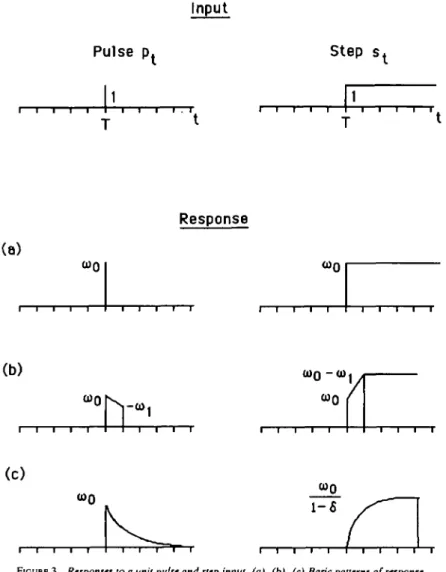
Other frequently arising problems concern 'changes' of time series. Changes may be expected after a 'man-made intervention' e.g. the introduction of a preven-tive programme. Alternapreven-tively changes may occur e.g. after an environmental accident. Characteristic properties of changes of series may be investigated by means of intervention analysis.' The following basic model has been used to represent the possible effect of a preventive measure on the number of injuries: y, = (o0sl+nt, with s, = fl for t=sT OforKT. (13) (14) The step function s, represents e.g. a preventive measure starting at time T. a»0 is a parameter (the height of the step etc.) which measures the size or strength of the effect, n, represents an ARIMA process as described above. Since n, may be non-stationary, large changes of the series could occur even when no preventive measure takes place.
Alternatively the dummy input variable may be a pulse function pt: y, = w0 pt+nt, where Pi = for t = T Oelse. (15) (16) The pulse function p, may represent e.g. an unusual event which acts only at time T.
Figure 3 shows basic intervention models. In the first line the two dummy input variables s, and p, are depicted. The lines (a), (b) and (c) below show responses corresponding to the models. Line (a) of
CCF * * • « • • « • • 1 • * t * 1 * t « « • • • • • • • • • • « • • • • • * • « • • • * * • « • « « * • « • * * * * * * * « • • • • t • « « * * * * • « * « • - 1 0 10 LAG PCCF « • * « - 1 0 1 0 LAG
FIGURE 2 Cross-correlation function between the series sulphur dioxide (SO^j (logarithmically transformed) and the series of symptoms, (a) Before
prewhitening (CCF). (b) After prewhitening (PCCF).
Figure 3 depicts the response corresponding to the above two models. In this case p, (respectively s,) is simply multiplied by co0.
It is possible that model (a) does not fully represent the characteristic properties of the series: with a step input the model predicts that the final level is reached immediately. However, it may be more realistic to con-sider the model in line (b) of Figure 3.
y, = (17)
Here the final level is reached in two steps. This model may give a better fit to the data (i.e. a smaller residual variance) than model (a). Figure 3(c) shows another possible type of response. The final level is reached only gradually. This model is represented by:
(18) Extensions of intervention models in many different directions are straightforward (compare last section). Of course it is desirable to include a comparison group (or area) with no intervention in the study design. Such studies have been performed e.g. in assessing the impact of preventive programmes (enforcement and media information campaign etc.) on the course of alcohol-related accidents."-20
FURTHER RELATED TIME SERIES METHODS The following example illustrates how forecasts may be calculated in a simple manner when an ARIMA model has been identified.
TIME SERIES METHODS IN EPIDEMIOLOGY Input 813 Pulse pt 1 Step st Response (a) (JUQ (b)
(0
conFIGURE 3 Responses to a unit pulse and sup input, (a), (b), (c) Basic patterns of response.
To obtain forecasts z,+, for 1 time units (days, months, etc.) ahead one has only to write the corre-sponding model equation by replacing (a) future values of the random shocks a by zero, (b) future values of z by the corresponding forecasts and (c) past values of z by their observed values. The following example may illustrate the simplicity of obtaining fore-casts e.g. for an AR(1) model:
<S>\ etc.
By continuing this procedure one may see that the forecasts corresponding to the AR(1) model follow an exponential curve.
Forecasts are not only of interest 'by itself. In
addi-tion, they provide a complementary way to investigate a possible change of a series.10 One may compare fore-casts arising from the pre-intervention series with actual data of the post-intervention series.
Both methods, intervention analysis and compari-son of forecasts with actual data assume that the time of the change is well known. However, when a preven-tive programme is started e.g. it is often not clear when it starts to show an effect. A modification of the inter-vention analysis allows the most likely time of change to be found. For each possible time an intervention analysis is performed (Box-Tiao stepping) and the corresponding residual variance is calculated. The most likely time is then the time instant which provides the best model i.e. the model with the smallest residual variance.21 A more advanced approach to identify such a 'change-point' may be found in Broemeling.22 In
studying the possible effect of preventive programmes it has been observed that the expected effect may pre-cede the actual time of intervention.21 It is possible as well that the effect shows up only after a certain delay time.
CONCLUDING REMARKS AND FURTHER READING SUGGESTIONS
The elaboration of models described in the preceding sections in many different directions is straightfor-ward. Intervention analysis with input consisting of multiple pulses for example may be used to analyse questions such as: Are there more deaths due to infarc-tion in years with influenza A than in years without? The sequence of pulses then represents years with influenza A.
Responses to an intervention need not to occur instantaneously. A preventive programme may show an effect eventually after a delay. Occasionally such programmes may show an effect even before the official programme is started. In such cases one may try to estimate a possible pre-intervention effect.21 In addition, effects of preventive programmes need not to show a permanent effect. Decomposing the dummy input in a short-term and a long-term component may help to decide if an effect is only transient.
Transfer function models and intervention analysis may be combined: Inversion of temperature for example may be represented by a dummy variable con-sisting of a sequence of 'ones' during the inversion pre-ceded and followed by 'zeros'. This 0/1-input may be used simultaneously with continuous inputs represent-ing e.g. concentrations of pollutants.
ARIMA models (and transfer function models) may be very useful for forecasting non-stationary series containing ordinary or seasonal trends. In particular, it may be possible to distinguish between models repre-senting deterministic and stochastic polynomial trends. In a deterministic trend model the coefficients of the polynomial are constant over time. In a stochas-tic trend model the coefficients are subject to random variation and the trend changes stochastically accord-ing to random shocks that enter the system.23
Thus, time series methods are suited to represent a large amount of relevant epidemiological problems. However, one should be aware of limitations which are naturally inherent to these methods. Gruchow etal.2*
studied relations between alcohol consumption and ischaemic heart disease by calculating CCFs. They came to the conclusion that 'time series correlations of aggregated data are not useful for the study of latency periods . . .'. This conclusion was drawn after calculat-ing CCFs between series containcalculat-ing trends, i.e.
non-stationary series. In order to get an interpretable CCF, the series have to be transformed to stationarity, i.e. the differencing operation has to be applied. Diffe-rencing eliminates trends; it has the effect of a high pass filter25 and the information contained in the low frequency range is lost. However the presence of domi-nating low frequencies may make it impossible to detect short-term correlations. Differencing thus may allow the detection of hidden relations in the high fre-quency range.26 It is also possible that the relation between two time series and the corresponding CCF change with time. In a study concerned with the assess-ment of relations between air pollutants and respir-atory symptoms it was found that the CCF may change with season. During the winter period an instan-taneous relation between the concentration of SO2 and the number of symptoms was identified but no such relation was found for the other seasons. Thus, it may be advisable to fit separate models to different sub-series (time splitting13).
It is important to mention that an alternative way of analysing time series data is based on the auto-spec-trum and on the cross-specauto-spec-trum instead of the ACF and the CCF. The auto-spectrum and the ACF (and the cross-spectrum and the CCF) are mathematically equivalent since they constitute a Fourier transform pair.1 However, they shed light on different comple-mentary aspects of time series data. The auto-spec-trum reveals which frequencies are present in an individual series and the cross-spectrum shows at which frequencies two series are related.27-28 Box and Jenkins1 use the ACF and not the auto-spectrum for the purpose of model identification because the par-simonious models they found to be useful in practice could be simply described in terms of the ACF.
Since the presentation in this article is necessarily short, the following suggestions for further' reading may be helpful.
An extensive introduction to ARIMA models and their identification may be found in 'The Analysis of Time Series: An Introduction'.25 A thorough presen-tation of transfer function models may be found in Chapter 8 of 'Statistical Methods of Forecasting',23 where forecasting is also discussed in depth.
For a deeper study of specific epidemiological time series problems the following articles are thought to be of particular interest. Analysis of relations between seasonal series is discussed in.I9J0 Identification of seasonal ARIMA models representing infectious dis-eases is presented in some detail in.31 Advantages of forecasting epidemiological series by means of ARIMA models over traditional methods are described in.32
TIME SERIES METHODS IN EPIDEMIOLOGY 815
Several investigators have used intervention analysis to assess changes of epidemiological series, in par-ticular to analyse the efficiency of preventive measures.33"33 A case study using intervention models to assess possible health effects of an environmental disaster may be found in.36 Comparison of forecasts with actual data has been used to study changes in the frequency of traditional neurological diagnostic methods after the introduction of computer tomography.37
REFERENCES
'BoxG EP, Jenkins GM. Time Series Analysis, Forecasting and
Con-trol, Revised Edition, San Francisco: Holden Day, 1976.
2 Armitage P. Statistical Methods in Medical Research, Oxford and
Edinburgh: Blackwell Scientific Publications, 1971; 347-48.
3 Katzoff M. The application of time series forecasting methods to an
estimation problem using provisional mortality statistics. Stat Med 1989; 8: 335-41.
* Schnell D, Zaidi A, Reynolds G. A time series analysis of gonorrhea surveillance data. Stat Med 1989; 8: 343-52.
1 Zaidi A, Schnell D, Reynolds G. Time series analysis of syphilis
sur-veillance data. Stat Med 1989; 8: 353-62.
6 Box G E P, Hunter W G, Hunter J S. Statistics for experimenters- An introduction to design, data analysis and model building, New
York: Wiley, 1978; pp 88-89.
7 Dixon W J (ed). BMDP Statistical Software, Berkeley: University of California Press, 1988.
1SAS Institute Inc SASIETS User's guide, version 5 edition. Cary, NC: SAS Institute Inc, 1984.
* Box G E P, Tiao G C. Intervention analysis with applications to econ-omic and environmental problems. J Am Stat Assoc 1975; 70: 70-9.
10 Box G E P, Tiao G C. Comparison of forecast and actuality. Appl Stat 1976; 25: 195-200.
" Tiao G C, Box G E P, Hamming W J. Analysis of Los Angeles photo-chemical smog data: A statistical overview. J Air Pollution Control Ass 1975; 25: 260-8.
a Ljung G M, Box G E P. On a measure of lack of fit in time series mod-els. Biometrika 1978; 65: 297-303.
u Jenkins G M. Practical Experiences with Modelling and Forecasting
Time Sena. St Helier: Gwilym Jenkins & Partners (Overseas) Ud, 1979; p 14.
" Bartlett M S. Some aspects of the time-correlation problem in regard to tesu of significance. / R Stat Soc 1935; 98: 536-43.
uB o x G E P, Newbold P. Some comments on a paper of Cohen,
Gomme and Kendall. J R Stat Soc A 1971; 134: 229-40. " Haugh L D. Checking the independence of two
covariance-station-ary time series: A univariate residual cross-correlation approach. J Am Stat Assoc 1976; 71: 378-85.
17 Haugh L D, Box G E P. Identification of dynamic regression
(distri-buted lag) models connecting two time series. J Am Stat Assoc 1977; 72: 121-30.
u Helfenstein U, Ackermann-Uebnch U, Braun-Fahrlander Ch,
Wanner H U. Air pollution and diseases of the respiratory tracts in pre-school children: A transfer function model. J
Environ Monitor Assess 1991; 17: (in press).
19 Sali G J. Evaluation of Boise selective traffic enforcement project.
Transportation Res Rep 1983; 910: 68-74.
20 Amick D R, Marshall P B. Evaluation of the Bonneville County, Idaho, DUI accident prevention program. Transportation Res Rep 1983; 910: 81-93.
n Helfenstein U. When did a reduced speed limit show an effect? Exploratory identification of an intervention time. Accident
Analysis & Prevention 1990; 22: 79-87.
B Broemeling L D. Bayesian Analysis of Linear Models. New York: Marcel Dekker, 1985; pp 308-12.
23 Abraham B, Ledolter J. Statistical Methods for Forecasting. New York: Wiley, 1983; pp 225-29, 336-55.
24 Gruchow H W, Rimm A A and Hoffmann R G. Alcohol consump-tion and ischemic heart disease mortality: Are time series cor-relations meaningful? Am J Epidemiol 1983; 118: 641-50.
23 Chatfield C. The Analysis of Time Series: An Introduction. London: Chapman and Hall, 1989; pp 27-65, 168-169.
26 Helfenstein U. Detecting hidden relations between time series of mortality rates. Methods of Information in Medicine 1990; 29: 57-60.
v Hoppenbrouwers T, Calub M, Arakawa K, Hodgman J E. Seasonal relationship of sudden infant death syndrome and environ-mental pollutants Am J Epidemiol 1981; 113: 623-35.
a Lebowitz M D, Collins L, Holberg C J. Time series analyses of res-piratory responses to indoor and outdoor environmental phenomena. Environ Res 1987; 43: 332-41.
29 Bowie C, ProtheroD: Finding causes of seasonal diseases using time series analysis. Int J Epidemiol 1981; 10: 87-92.
30 Murphy M F G, Campbell M J. Sudden infant death syndrome and environmental temperature: an analysis using vital statistics. J
Epidemiol Community Health 1987; 41: 63-71.
31 Helfenstein U. Box-Jenkins modelling of some viral infectious
dis-eases Statistics in Medicine 1986, 5: 37-47.
33 Choi K, Thacker S B. An evaluation of influenza mortality sur-veillance, 1962-1979. I. Time series forecasts of expected pneumonia and influenza deaths. Am J Epidemiol 1981; 13: 215-26.
33 Bhattacharyya M N, Layton A P. Effectiveness of seat belt legis-lation on the Queensland Road Toll. An Australian case study in intervention analysis. J Am Stat Assoc 1979; 74: 596-603. M Lassare S, Tan S H. Evaluation of safety measures on the frequency
and gravity of traffic accidents in France by means of interven-tion analysis. In: Anderson O D (ed) Time series Analysis, Theory and Practice I, North-Holland Publishing Company, 1982; pp 297-306.
33 Martinez-Schnell B, Zaidi A. Time series analysis of injuries.
Statis-tics in Medicine 1989; 8: 1497-508.
36 Helfenstein U, Ackermann-Liebrich U, Braun-Fahrlander Ch, Wanner H U. The environmental accident of 'Schweizerhalle' and respiratory diseases: A time series analysis. 1991; Statistics in Medicine 1991; 10 (In Press).
37 Tsouros A D, Young R J. Applications of time series analysis: A case study on the impact of computer tomography. Statistics in Medicine 1986; 5: 593-606.